Chiral Extension of Lattice Gauge Theory

Abstract

Two approaches are presented to coupling explicit Goldstone modes to $N_{f}$ flavors of massless quarks preserving exact $SU(N_{f})\times SU(N_{f})$ chiral symmetry on the lattice. The first approach is a generalization a chiral extension to QCD (aka XQCD) proposed by Brower, Shen and Tan consistent with the Ginsparg-Wilson relation. The second approach based on the Callan, Coleman, Wess and Zumino coset construction has a real determinant at zero quark axial coupling, $g_{A}=0$.

1 INTRODUCTION

A persistent difficulty with the standard lattice approach to low energy hadronic processes is the difficulty with small eigenvalues in the limit of small quark mass, which through the Banks-Cashir formula are responsible for chiral symmetry breaking. Since these eigenvalues are represented faithfully by bosonic matrix models, one might hope that they could somehow be “bosonized”. In 1994, Brower, Shen and Tan [1] introduced a new methods called “chirally extended QCD” (or $XQCD$) in this spirit. The lattice action is modified by adding explicit fields for the Goldstone modes that has the effect of replacing the low eigenvalues by a constituent quark mass $M_{Q}$ without explicitly breaking $SU_{L}(N_{f})\times SU_{R}(N_{f})$ chiral symmetry.

Here we extend this method to incorporate chiral fermions obeying the Wilson-Ginsparg relation. In this way we believe the continuum limit for XQCD on the lattice will approach the universal fixed point for QCD without fine tuning. These methods are of general interest for the study of non-perturbative models of chiral symmetry and Higgs symmetry breaking phenomena on the lattice.

2 LATTICE REALIZATIONS

In continuum notation, the Lagrangians we wish to put on the lattice have the general form,

$${\cal L}_{\chi QCD}={\cal L}_{YM}+{\cal L}_{\chi}+{\cal L}_{F}\;,$$ (1)

where the Yang Mills theory and non-linear chiral Lagrangian for the Goldstone modes

$${\cal L}_{YM}=\frac{1}{4}Tr[F^{2}_{\mu\nu}]\quad\mbox{and}\quad{\cal L}_{\chi}=\frac{F^{2}_{\pi}}{4}\mbox{Tr}[\partial_{\mu}\Sigma^{2}]+\cdots$$ (2)

respectively are coupled through Yukawa interactions in the Fermion action,

$${\cal L}_{F}=\bar{\psi}\gamma_{\mu}(\partial_{\mu}-ig_{YM}A_{\mu})\psi+M_{Q}\bar{\psi}\Sigma^{(5)}\psi\;.$$ (3)

Here $\Sigma$ is an element of $SU(N_{f})$ and we define

$$\Sigma^{(5)}\equiv\frac{1+\gamma_{5}}{2}\Sigma+\frac{1-\gamma_{5}}{2}\Sigma^{\dagger}\equiv\exp[2i\gamma_{5}\vec{\pi}\cdot\vec{\tau}/F_{\pi}]\;.$$ (4)

One can place this on a lattice by introducing a naive Fermions action

$$S_{F}={\scriptstyle\frac{1}{2}}\bar{\Psi}_{x}[\gamma_{\mu}U_{\mu}(x)\delta_{x+1,y}-\gamma_{\mu}U^{\dagger}(x)\delta_{x,y+1}]\Psi_{y}$$ (5)

plus a Wilson-Yukawa term that removes doublers and respects chiral invariance:

$$\bar{\Psi}_{x}[\frac{r}{2}(\delta_{xy}-U_{\mu}(x)\delta_{x+1,y}-U^{\dagger}(x)\delta_{x,y+1})$$

$$\qquad(\Sigma^{(5)}_{x}+\Sigma^{(5)}_{y})+(M_{Q}\Sigma^{(5)}_{x}+m_{q})\delta_{xy}]\Psi_{y}\;.$$

The only term that explicitly breaks $S(N_{f})\times SU(N_{f})$ symmetry is the quark mass term, $m_{q}\bar{\Psi}_{x}\Psi_{x}$. Still if there is a continuum limit which decouples the scaler fields, a delicate fine tuning must be required to adjust the renormalized quark mass to zero. To avoid this problem we now consider coupling to Ginsparg-Wilson fermions.

2.1 Overlap Fermions

With the standard overlap operator, $D_{0}=1+\gamma_{5}\epsilon(H_{W})$, the Ginsparg-Wilson relation can be express in two alternative (asymmetric) forms,

$$\gamma_{5}D_{0}+D_{0}\widehat{\gamma}_{5}=0\quad\mbox{and}\quad\widehat{\gamma}^{\prime}_{5}D_{0}+D_{0}\gamma_{5}=0$$ (6)

with $\widehat{\gamma}_{5}\equiv\gamma_{5}(2-D_{0})$ and $\widehat{\gamma}^{\prime}_{5}\equiv(2-D_{0})\gamma_{5}$ respectively. Thus there are two different realizations of lattice chiral symmetry with non-local projectors $1\pm\widehat{\gamma}_{5}$ or $1\pm\widehat{\gamma}^{\prime}_{5}$ acting on the “ket’s” or “bra’s”respectively. This leads to two ways to embed the chiral extension into the Ginsparg-Wilson relation. We will show that they are both equivalent up to a field redefinition and indeed both can be derived from a single form of the Domain Wall action.

The construction is straight forward. In the first case the chiral transformations become,

$$\Psi \rightarrow \exp[i\widehat{\gamma}_{5}\vec{\theta}_{A}\cdot\vec{\lambda}+i\vec{\theta}_{V}\cdot\vec{\lambda}]\Psi$$

$$\bar{\Psi} \rightarrow \bar{\Psi}\exp[i\gamma_{5}\vec{\theta}_{A}\cdot\vec{\lambda}-i\vec{\theta}_{V}\cdot\vec{\lambda}]$$ (7)

The invariant Fermion term is

$$\bar{\Psi}_{x}D_{0,x,y}\Psi_{y}+M_{Q}[\bar{\Psi}_{L,x}\Sigma_{x}\Psi_{R,x}+\bar{\Psi}_{R,x}\Sigma^{\dagger}_{x}\Psi_{L,x}]$$

or a new XQCD operator,

$$D(U,\Sigma)=D_{0}(U)+M_{Q}\Sigma^{(5)}(1-D_{0}(U))\;.$$ (8)

Expanding $\Sigma^{(5)}=\widehat{\sigma}(x)+i\gamma_{5}\vec{\tau}\cdot\vec{\widehat{\pi}}(x)$ for $N_{f}=2$, we have rather familiar looking form,

$$D(U,\Sigma)=D_{0}+M_{Q}\widehat{\sigma}\frac{1+\gamma_{5}\widehat{\gamma}_{5}}{2}+iM_{Q}\vec{\tau}\cdot\vec{\widehat{\pi}}(x)\frac{\gamma_{5}+\widehat{\gamma}_{5}}{2}\;.$$

The alternative form is

$$\widetilde{D}(U,\Sigma)=D_{0}+M_{Q}(1-D_{0})\Sigma^{(5)}$$ (9)

One readily shows that the measure preserving field redefinition $\Psi_{x}\rightarrow\Psi^{\prime}_{x}=(1-D_{0})\Psi_{x}$, and $\bar{\Psi}_{x}\rightarrow\bar{\Psi}^{\prime}_{x}=\bar{\Psi}_{x}(1-D_{0})^{-1}$ converts one form into the other.

2.2 Coset Construction

The coset construction for the chiral breaking of a symmetry group G to a subgroup H, fixes the frame Fermion field, $\Psi_{x}=\gamma(x)Q_{x}$, by choosing a canonical element $\gamma(x)$ in the coset G/H. In our present case, the natural choice is

$$\gamma(x) = \xi^{(5)\dagger}\equiv\exp[-i\gamma_{5}\vec{\pi}\cdot\vec{\tau}/F_{\pi}]$$ (10)

$$= {\scriptstyle\frac{1}{2}}(1+\gamma_{5})\xi^{\dagger}+{\scriptstyle\frac{1}{2}}(1-\gamma_{5})\xi\;.$$

Now chiral symmetry requires a rotation of the new quark field $Q_{x}$ to re-establishes the frame: $Q_{x}\rightarrow u_{x}Q_{x}\quad\mbox{,}\quad\bar{Q}_{x}\rightarrow\bar{Q}_{x}u^{\dagger}(x)$, when $\xi_{x}\rightarrow L\xi_{x}u^{\dagger}(x)=u(x)\xi_{x}R^{\dagger}$.

There are a variety of ways to proceed to construction invariant lattice Lagragians. One nice way is to introduce bilocal lattice “currents”: $j_{R}=\xi^{(5)}_{x}\xi^{\dagger(5)}_{y}=V_{xy}+i\gamma_{5}A_{xy}$ and $j_{L}=\xi^{\dagger(5)}_{x}\xi^{(5)}_{y}=V_{xy}-i\gamma_{5}A_{xy}$ where $V_{xy}=\frac{1}{2}(\xi^{\dagger}_{x}\xi_{y}+\xi_{x}\xi^{\dagger}_{y})\quad\mbox{and}\quad A_{xy}=\frac{1}{2i}(\xi^{\dagger}_{x}\xi_{y}-\xi_{x}\xi^{\dagger}_{y})$ transform as adjoint flavor tensors: $V_{xy}\rightarrow u_{x}V_{xy}u_{y}^{\dagger}$, $A_{xy}\rightarrow u_{x}A_{xy}u_{y}^{\dagger}$. Now the Fermion operator takes the attractive from, $D^{coset}_{xy}(U,\xi)=D_{0xy}(V_{xy}+ig_{A}A_{xy})$, leading to a general lattice action,

$$S_{XQCD} = \!\!\!\!\frac{6}{g^{2}_{0}}Tr[U_{\mu\nu}]+\bar{Q}_{x}D^{coset}_{xy}(U,\xi)Q_{y}$$

$$+ \!\!\!\!M_{Q}\bar{Q}_{x}Q_{x}+{\scriptstyle\frac{1}{2}}m_{q}\bar{Q}_{x}\xi^{\dagger(5)}_{x}\xi^{\dagger(5)}_{x}Q(x)$$

$$+ \!\!\!\!\frac{F_{\pi}}{4}\sum_{x,\mu}Tr[A(x,x+\mu)A^{\dagger}(x,x+\mu)]$$

where the kinetic term for the non-linear sigma models again is rewritten by $Tr[A_{x,x+\mu}A^{\dagger}_{x,x+\mu}]\\ =\frac{1}{4}Tr[(\Sigma_{x+\mu}-\Sigma_{x})(\Sigma^{\dagger}_{x+\mu}-\Sigma^{\dagger}_{x})]$.

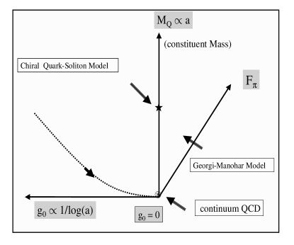
Figure 1: Renormalization group flow at zero quark mass $m_{q}$

3 DISCUSSION

More details will be given in a forth coming publication by Berruto, Brower, Neff, Edwards, Lim and Tan. However there are several remarks that should be made.

As emphasized recently by Chandrasekharan, Pepe, Steffen and Wiese [2] the coset construction applies to very wide class of effective chiral Lagragians. For example one can replace the overlap operator $D_{0}$ above by the standard Wilson lattice operator, still maintaining exact $SU(N_{f})\times SU(N_{f})$ up to explicit quark mass terms. Indeed the value of $g_{A}$ maybe different in the naive kinetic term and the Wilson mass term and setting them to $g_{A}=1$ and $g_{A}=0$ respectively gives precisely the original Wilson-Yukawa construction with the field redefinition $Q_{x}\rightarrow\xi^{(5)}\Psi_{x}$. The most general clover improved XQCD (i.e. using all 5-d operators) will be given elsewhere.

In general these action lead to a complex determinant. Indeed using the gradient expansion for weak fields one can show that first contribution to the phase linear in $g_{A}$ is proportional to 13-d operators such as:

$$\frac{g_{A}g^{3}}{m_{Q}^{6}}\ \epsilon_{ijk}\partial^{2}_{\lambda}\pi^{i}\partial_{\mu}\pi^{j}\partial_{\nu}\pi^{k}d_{abc}F_{\mu\nu}^{a}F_{\rho\tau}^{b}\widetilde{F}_{\rho\tau}^{c}$$

This is consistent with general theorems for a vanishing phase with $N_{c}\leq 2$ or $N_{f}<2$ or $d\leq 3$ or $g_{A}=0$, etc.

Finally the general form of our Lagrangian for XQCD has 3 basic parameters: the bare gauge coupling,$g_{0}$, the constituent quark mass $F_{\pi}$ and the bare pion decay constant $F_{\pi}$ (see Fig. 1). Special limits afford interesting models. The Georgi-Manohar chiral quark model is $g_{0}\rightarrow 0$, which reproduces the non-relativistic quark model results with $g_{A}\simeq 0.75$ and $M_{Q}\simeq 350Mev$. The Chiral Soliton Quark model,which is believed to have proton and Delta bound states is $F_{\pi}\rightarrow 0$,$g_{0}\rightarrow 0$. These non-linear effective chiral lattice actions will allow a non-perturbative investigation of the phase diagram (Fig. 1) to clarify chiral symmetry breaking mechanism in general and the best way to approach the chiral limit of QCD in particular.

References

• [1] R. C. Brower, Y. Shen and C-I Tan, ”Chirally Extended Quantum Chromodynamics”, Int.J.Mod.Phys. C6 (1995) 725.
• [2] S. Chandrasekharan, M. Pepe, F. D. Steffen and U-J. Wiese ”Nonlinear realization of chiral symmetry on the lattice” hep-lat/0306020 (2003).