Electromagnetic Hadronic Form-Factors

Abstract

We present a calculation of the nucleon electromagnetic form-factors as well as the pion and rho to pion transition form-factors in a hybrid calculation with domain wall valence quarks and improved staggered (Asqtad) sea quarks.

The determination of light hadron physics properties is of considerable interest to experimental labs such as Jefferson Lab. Many quantities, such as hadron form-factors and generalized structure functions, are not well understood theoretically. The available and forthcoming high precision experimental data presents considerable challenges and many opportunities for corresponding lattice calculations. Including the contribution of light dynamical quarks is an important goal of this work, but the cost of generating these gauge ensembles is large. We have adopted a so-called “hybrid” scheme where staggered sea quarks are used (Asqtad action [1]) and domain wall valence quarks [2]. While unitarity is broken at finite lattice spacing, it is recovered in the continuum limit when the sea and valence quark masses are properly tuned.

In this contribution, we study the efficacy of an uncommon method of calculating three-point functions that avoids sequential source techniques. We calculate various electro-magnetic form-factors without the cost of a new sequential inversion for each new set of observables. The method is particularly suitable for valence quark actions amenable to a multi-mass solver, such as the Overlap quark action. The conclusion is that the method appears viable, but very light quark mass tests are needed (and on-going).

A typical sequential source method for computing a matrix element such as $\langle B(p_{f})|V(q)|A(p_{i})\rangle$ for an initial state $A$ with three-momenta $p_{i}$ and final state $B$ at momenta $p_{f}$ with a two-quark insertion $V$ involves either a sequential inversion through the insertion or the sink. To properly extract the matrix element for a set of momenta $q=p_{f}-p_{i}$, usually the sequential source for the sequential insertion is held at a fixed momenta. There are two common techniques. Sequential inversion through insertion: benefits are that one can vary the source and sink fields but the insertion momenta and operator are fixed. Sequential inversion through sink: benefits are one can vary the insertion operator and momenta, but the sink operator and momenta are fixed. In addition, for baryons the spin projection matrix between the source and sink must be fixed necessitating different sequential inversions to extract electric and magnetic quantities. The common problem is one vertex must have a definite momentum.

As an alternative, one can instead make a sink (or source) quark propagator (as opposed to the state) have a definite momentum. Putting the sink (or source) quarks at definite momentum implies the hadron state has a fixed momenta via the translation/momentum operator on the lattice. The scheme then is to build the desired hadron state propagating from the source and sink where the quark propagators used for one of these states has a fixed momenta. Thus, one avoids sequential inversions computing $\langle B(p_{f})|V(q)|A(p_{i})\rangle$. For example, fixing the sink momenta to a fixed $p_{f}$, one can extract the matrix element at all $q$ by vary $p_{i}$ according to momentum conservation.

To fix a quark’s momenta necessarily implies a wall source thus requiring the need for gauge fixing. Additional tricks can be used to improve statistics like using charge conjugation and time reversal (CT) in (anti-)periodic boundary conditions. This method also works for Dirichlet boundary conditions where one maintains equal source and sink separation from the Dirichlet wall. E.g., a wall sink hadron because a wall source after CT. If applicable, multi-mass inversion techniques can be applied both to the source and the sink propagator calculations.

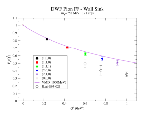
Figure 1: Pion electromagnetic form-factor computed by Eq. 1 and imposing the lattice dispersion relation.

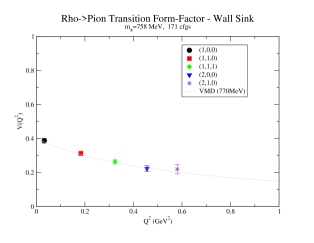
Figure 2: $\rho\rightarrow\pi$ transition form-factor. The VMD line has a 0.4 normalization.

For our calculation of hadronic form factors with unquenched gauge configurations, we performed a hybrid calculation using MILC $N_{f}=2+1$ configurations in 20${}^{3}\times$64 volumes, generated with staggered asqtad sea quarks[1], and domain wall valence quarks with domain wall height $m_{0}=1.7$ and extent $L_{s}=16$ of the extra dimension [2]. The MILC configurations were HYP blocked [3] before valence propagators were computed, otherwise the residual chiral symmetry breaking would have been unacceptably large. Dirichlet boundary conditions were imposed 32 time slices apart. The lattice spacing scale is set at $a=0.125$fm. The Asqtad set has $m_{u}=0.01$ and $m_{s}=0.05$, $\beta=6.76$. The valence pion and rho mass are $m_{\pi}=758(5)$MeV and $m_{\rho}=1060(14)$MeV, resp.

The technique for extracting form factors uses the ratio method of correlation functions:

$$R^{XY}_{\alpha\beta\mu}=\frac{\Gamma_{\alpha\beta,\mu,AB}^{XY}(t_{i},t,t_{f},\vec{p}_{i},\vec{p}_{f})\Gamma_{CL}^{YY}(t_{i},t,\vec{p}_{f})}{\Gamma_{AL}^{XX}(t_{i},t,\vec{p}_{i})\Gamma_{CB}^{YY}(t_{i},t_{f},\vec{p}_{f})}$$ (1)

where $A$, $B$, $C$ are generic smearing labels, $L$ is local and $\mu$ is the direction of the local current, the initial and final states are $X_{\alpha}$ and $Y_{\beta}$. Similarly for $R^{YX}=R^{XY}$ where $Y\rightarrow X$ . Note, momenta and smearing labels are not interchanged. In the case of $Y=X$, this ratio cancels all wave-function factors and exponentials. For the transition case, the combination $(R^{YX}R^{XY})^{1/2}$ cancels all exponentials and wave-function factors taking into the effects of smearing on the wave-functions. One extracts the form-factors up to some kinematic factors using properties of the spin projection matrix between $X_{\alpha}$ and $Y_{\beta}$. In all the subsequent work, we fixed the wall sink to have $\vec{p}_{f}=0$. The source quarks are APE smeared.

The first test of the wall-sink method involves the pion form factor. The result shown in Fig. 1 compares favorably with a sequential-sink technique [4] at the one mass in common corresponding to $am_{\rm val}=0.081$. The obtained value of $Z_{V}$ for our local current also agrees well.

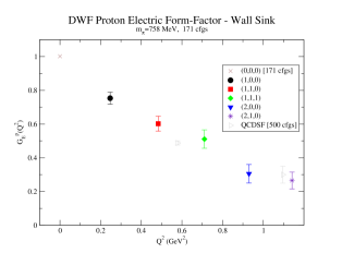
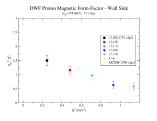
Figure 3: Proton electric and magnetic form factors. Also shown are results from QCDSF [7].

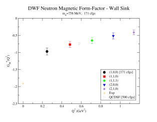
Figure 4: Neutron magnetic form-factor.

Electro-disintegration of the deuteron has been intensively studied experimentally. While isovector meson exchange currents have been identified in such systems, the role of isoscalar meson exchange is not clear. Here, we provide a lattice measurement of the $\rho\rightarrow\pi$ transition form factor which is an important step in an analysis of exchange mechanisms. The matrix element computed is

$$Z_{V}\left<\pi(\vec{p}_{f})\left|V_{\mu}(0)\right|\rho(\vec{p}_{i},r)\right>\\ =\frac{2V(Q^{2})}{m_{\pi}+m_{\rho}}\epsilon^{\mu\alpha\delta\beta}p_{\alpha,f}p_{\delta,i}\epsilon_{\beta}(\vec{p}_{i},r)$$

The form factor $V(Q^{2})$ shown in Fig. 2 is in rough agreement with a phenomenological calculation in Ref. [5]. The coupling constant normalization taken from $V(0)$ is in rough agreement with experiment Ref. [6, 5]. Higher $Q^{2}$ are needed.

The extraction of the proton and neutron form factors uses Eq. 1 together with a spin projection matrix $T_{\alpha\beta}$ between source and sink nucleon states $N_{\alpha}$ and $N_{\beta}$. We can increase statistics on the electric and magnetic form-factors by averaging over all the nucleon spin polarizations. The results for the proton and neutron are shown in Figs. 3 and 4. Compared with quenched clover results from QCDSF [7] at roughly the same pion mass ($\beta=6.0$, $\kappa=0.1338$), the error bars stay somewhat constant at higher $Q^{2}$. Reasonable agreement is seen with experiment and Ref. [7]. In addition, a signal is seen for the computationally difficult neutron electric form-factor.

This work was supported by the U.S. Department of Energy under contract DE-AC05-84ER40150. Computations were performed on the Pentium IV clusters at JLab.

References

- [1] C.W. Bernard et al., Phys. Rev. D64 (2001) 054506, hep-lat/0104002.
- [2] LHPC: J.W. Negele et al., Nucl. Phys. Proc. Suppl. 128 (2004) 170, hep-lat/0404005.
- [3] A. Hasenfratz and F. Knechtli, Phys. Rev. D64 (2001) 034504, hep-lat/0103029.
- [4] LHPC, F. Bonnet et al., hep-lat/0310053.
- [5] H. Ito and F. Gross, Phys. Rev. Lett. 71, 2555 (1993).
- [6] D. Berg, et al., Phys. Rev. Lett. 44, 706 (1980).
- [7] M. Göckeler, et al., hep-lat/0303019.