Chiral perturbation theory for twisted mass QCD

Abstract

Quantum Chromodynamics on a lattice with Wilson fermions and a chirally twisted mass term for two degenerate quark flavours is considered in the framework of chiral perturbation theory. The pion masses and decay constants are calculated in next-to-leading order including terms linear in the lattice spacing $a$. We treat both unquenched and partially quenched QCD. We also discuss the phase structure of twisted mass lattice QCD.

1 Introduction

Lattice QCD is fighting on several fronts in order to obtain results relevant to the physics of hadrons in the continuum: one wants to control the effects (a) of the finite size of the lattice, (b) of the non-zero lattice spacing $a$, and (c) of too large quark masses. For small quark masses Monte Carlo calculations suffer from a slowing down roughly proportional to $m_{q}^{p}$ with $p=2-3$. This has so far prevented simulations with light Wilson quarks of realistic masses.

For the extrapolation of the numerical results to small values of up- and down-quark masses, chiral perturbation theory can be employed. It amounts to an expansion around the chiral limit at vanishing quark masses. The low energy parameters of chiral perturbation theory, the Gasser-Leutwyler coefficients, can in turn be determined by numerical simulations of lattice QCD, see [1] for a review.

1.1 Twisted mass lattice QCD

For simplicity we consider QCD with $N_{f}=2$ flavours of degenerate light quarks, $m_{u}=m_{d}$, in the following. Consider a “twisted” quark mass matrix ($\tau_{3}$ acts in flavour space)

$$M(\omega)=m_{q}\,\mathrm{e}\,^{\mathrm{i}\,\omega\gamma_{5}\tau_{3}}=m+\mathrm{i}\,\mu\gamma_{5}\tau_{3}\,,$$

where $m=m_{q}\cos(\omega),\ \mu=m_{q}\sin(\omega)$. In the continuum the angle $\omega$ can be removed by a chiral rotation $q=\mathrm{e}\,^{-\mathrm{i}\,\omega\gamma_{5}\tau_{3}/2}q^{\prime}$, so that physics does not depend on $\omega$. On the lattice, however, chiral symmetry is broken even for massless QCD, and there is a dependence on $\omega$ due to lattice artifacts. Twisted mass lattice QCD has been introduced in [2]. Recently it has been advocated to employ a chirally twisted quark mass matrix for Wilson fermions in order to improve the efficiency of QCD simulations due to full $\mathcal{O}(a)$ improvement occurring for $\omega=\pi/2$ [3].

1.2 Chiral perturbation theory

The $\textrm{SU}(N_{f})_{L}\otimes\textrm{SU}(N_{f})_{R}$ chiral symmetry of massless QCD is spontaneously broken to $\textrm{SU}(N_{f})_{V}$, and in addition explicitly broken by non-vanishing quark masses. For $N_{f}=2$ the corresponding Pseudo-Goldstone bosons are the pions $\pi_{b}$. Chiral perturbation theory describes their dynamics by means of a low-energy Lagrangian. It is expressed in terms of the matrix-valued field $U(x)=\exp(\mathrm{i}\,\,\pi_{b}(x)\tau_{b}/F_{0})$, which transforms as $U\rightarrow LUR^{-1}$ under chiral transformations $(L,R)\in\textrm{SU}(N_{f})_{L}\otimes\textrm{SU}(N_{f})_{R}$.

The leading order effective Lagrangian is

$$\mathcal{L}_{2}=\frac{F_{0}^{2}}{4}\,\mbox{Tr}\left(\partial_{\mu}U^{\dagger}\,\partial^{\mu}U\right)-\frac{F_{0}^{2}}{4}\,\mbox{Tr}\left(\chi U^{\dagger}+U\chi^{\dagger}\right),$$

where the quark masses are contained in the matrix $\chi=2B_{0}m\,{\bf 1}$. In higher orders, terms with more fields and/or derivatives appear, which are multiplied by the Gasser-Leutwyler coefficients.

1.3 Chiral perturbation theory for lattice QCD

Chiral perturbation theory can also be applied to QCD on a lattice, see Oliver Bär’s talk at this conference. The fields of the low-energy effective Lagrangian are still defined in the continuum, but the lattice artifacts are taken into account by additional terms in $\mathcal{L}$ proportional to powers of $a$ [4, 5]. Physical quantities, like $m_{\pi}^{2}$ and $F_{\pi}$, appear in double expansions in quark masses (modified by logarithms) and in $a$. In leading order the lattice terms read $\mathcal{L}_{2L}=-(F_{0}^{2}/4)\,\mbox{Tr}\,(\rho\,U^{\dagger}+U\rho^{\dagger})$, where $\rho=2W_{0}a\,{\bf 1}$, with a new parameter $W_{0}$. Next-to-leading order calculations have been done in [5] up to $\mathcal{O}(a)$ and in [6] up to $\mathcal{O}(a^{2})$.

2 Chiral perturbation theory for twisted mass lattice QCD

In view of Monte Carlo calculations in twisted mass lattice QCD, it is desirable to extend chiral perturbation theory to this case. This has been done in [7]. The twisting of the mass term $\chi\to\chi(\omega)=2B_{0}m_{q}\,\mathrm{e}\,^{-\mathrm{i}\,\omega\tau_{3}}$ can be shifted to the lattice term by a chiral rotation $\rho\to\rho(\omega)=\mathrm{e}\,^{\mathrm{i}\,\omega\tau_{3}}\rho$.

In leading and next-to-leading order (NLO) the Lagrangian correspond to the one of [5] with a twisted lattice term $\rho(\omega)$. Spurion analysis shows that the twisting of the mass term does not produce further terms.

The vacuum corresponds to the minimum of $\mathcal{L}$. In contrast to the untwisted case, the minimum of the effective action is not located at vanishing fields, but at a point where $\pi_{3}\neq 0$, displaying an explicit flavour and parity breaking. Chiral perturbation theory amounts to an expansion around this shifted vacuum.

2.1 Pion mass and decay constant

Expansion of $\mathcal{L}$ in terms of pion fields yields the tree level contribution to the pion propagator. Loop contributions come from the leading order vertices. New vertices arising from the shift of the vacuum yield contributions at order $a^{2}$ only. As a result we obtain
$m_{\pi}^{2}=\chi_{0}+\rho_{0}+8(\chi_{0}^{2}/F_{0}^{2})(4L_{6}^{r}+2L_{8}^{r}-2L_{4}^{r}-L_{5}^{r})$
$+8(\chi_{0}\rho_{0}/F_{0}^{2})(4W_{6}^{r}+2W_{8}^{r}-2W_{4}^{r}-W_{5}^{r}-2L_{4}^{r}-L_{5}^{r})$
$+((\chi_{0}+\rho_{0})^{2}/(32\pi^{2}F_{0}^{2}))\,\ln((\chi_{0}+\rho_{0})/\Lambda^{2})\,,$
where $\chi_{0}=2B_{0}m_{q}\,,\ \rho_{0}=2W_{0}a\,\cos(\omega)$. Here $L_{k}^{r}$ and $W_{k}^{r}$ are renormalized chiral parameters and $\Lambda$ is the renormalization scale.

At order $a$, the dependence on the twist angle $\omega$ shows up in factors $\cos(\omega)$. It should be noted, however, that this is different in higher orders, where the above mentioned shift in the pion fields introduces new vertices.

In the case of maximal twist, $\omega=\pi/2$, the lattice artifacts vanish to order $a$. This has been observed for lattice QCD in general in [3], and is the basis of the improvement proposal made there.

The second physical quantity we calculated is the pion decay constant $F_{\pi}$, given by $\langle 0|J_{A}^{\mu,a}|\pi_{b}(p)\rangle=\mathrm{i}\,F_{\pi}p^{\mu}\delta_{ab}$, where $J_{A}$ is the axial current. A one-loop calculation gives
$F_{\pi}=F_{0}(1+(4/F_{0}^{2})[\chi_{0}\,(2L^{r}_{4}+L^{r}_{5})+\rho_{0}\,(2W_{4}^{r}$
$+W_{5}^{r})]-(1/16\pi^{2}F_{0}^{2})[(\chi_{0}+\rho_{0})\ln((\chi_{0}+\rho_{0})/\Lambda^{2})]).$

3 Partially quenched lattice QCD

Partially quenched QCD is an algorithmic approach to the regime of small quark masses. The Monte Carlo updates are being made with sea-quarks, which have large enough masses $m_{S}$ in order to allow a tolerable simulation speed. On the other hand, quark propagators and related observables are evaluated with smaller valence-quark masses $m_{V}$. Chiral perturbation theory has been adopted to the case of partially quenched QCD in [8, 9].

Combining the approaches mentioned above, it appears attractive to simulate QCD with chirally twisted quark masses in a partially quenched manner. For the theoretical analysis of the data the extension of the results of [7] to the partially quenched case has been done in [10].

In partially quenched chiral perturbation theory the field $U(x)$ is extended to a graded matrix in $\textrm{SU}(4|2)$. The quark mass matrix is in our case given by $M=\mbox{diag}(m_{V},m_{V},m_{S},m_{S},m_{V},m_{V})$. Its twisted counterpart is $M(\omega_{V},\omega_{S})=M\,\mathrm{e}\,^{\mathrm{i}\,\omega_{V}\tau_{3}^{V}\gamma_{5}}\ \mathrm{e}\,^{\mathrm{i}\,\omega_{S}\tau_{3}^{S}\gamma_{5}}\ \mathrm{e}\,^{\mathrm{i}\,\omega_{V}\tau_{3}^{G}\gamma_{5}}$.

We have calculated the pion masses $m_{SS}$, $m_{VV}$, $m_{VS}$ and decay constants $F_{SS}$, $F_{VV}$ and $F_{VS}$ at NLO (one-loop) including $\mathcal{O}(a)$ [10]. At order $a$ the dependence on the twist angle amounts to factors $\cos\omega_{V}$ or $\cos\omega_{S}$. The expressions can be used in the analysis of numerical results from Monte Carlo calculations and will aid the extrapolation to small quark masses.

An extension of the calculation to order $a^{2}$ is in progress. For the unquenched case results have been published recently by Scorzato [11] and Sharpe and Wu [12, 13].

4 Phase structure of twisted mass QCD

A prerequisite to any numerical simulation project is the knowledge of the phase structure of the model under consideration. Where are lines or points of phase transitions and how do physical quantities like particle masses behave near them? The phase structure of twisted mass lattice QCD has been discussed in [14, 11, 12, 13] on the basis of chiral perturbation theory.

For lattice QCD without twist, Aoki has proposed the possibility of a phase with spontaneous flavour and parity breaking [15]. An analysis of this scenario based on chiral perturbation theory has been made by Sharpe and Singleton [4]. A central role plays the potential $V=-c_{1}\,u_{0}+c_{2}\,u_{0}^{2}$ contained in the effective Lagrangian, where $u_{0}=\frac{1}{2}\mbox{Tr}(U)$. It contains parameters $c_{1}\sim m_{q},\ c_{2}=\mathcal{O}(a^{2})$ for small $m_{q}=\mathcal{O}(a^{2})$.

In twisted mass QCD, where $\mu=m_{q}\sin(\omega)\neq 0$, the potential $V$ gets additional contributions: $V=-c_{1}\,u_{0}+c_{2}\,u_{0}^{2}+c_{3}\,u_{3}$, where $c_{3}=2F_{0}^{2}B_{0}\,\mu\,,\ u_{3}=\frac{1}{2\mathrm{i}\,}\mbox{Tr}(\tau_{3}U)$.

Depending on the sign of $c_{2}$, the possible scenarios are

$c_{2}>0$ : Aoki scenario near the “critical hopping parameter” $\kappa_{c}$ with explicit flavour and parity breaking, and massive pions.

$c_{2}<0$ : normal scenario with a 1${}^{\mbox{st}}$ order phase transition extending into the $\mu\neq 0$ region, with a second order end point at $\mu_{c}=|c_{2}|/F_{0}^{2}B_{0}\sim a^{2}$.

On the phase transition line the jump in the quark condensate and the neutral pion mass decrease to zero, when the endpoint is approached: $(\Delta<\bar{\chi}\chi>)^{2}\sim m_{\pi 3}^{2}=(1/2F_{0}^{2}|c_{2}|)(4c_{2}^{2}-c_{3}^{2})\sim a^{2}$.

Recent Monte Carlo calculations [16, 17] at $\beta=5.2$ indicate the presence of the normal scenario with a first order line. Owing to the associated two-phase coexistence and metastability, this represents a problem for numerical simulations and it would be desirable to have the phase transition line as short as possible.

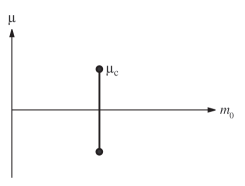
Figure 1: Phase structure for the normal scenario

References

- [1] H. Wittig, Nucl. Phys. B (Proc. Suppl.) 119 (2003) 59.
- [2] R. Frezzotti, P.A. Grassi, S. Sint and P. Weisz, Nucl. Phys. B (Proc. Suppl.) 83 (2000) 941; JHEP 0108 (2001) 058.
- [3] R. Frezzotti and G.C. Rossi, JHEP 0408 (2004) 007.
- [4] S. Sharpe and R. Singleton, Phys. Rev. D 58 (1998) 074501.
- [5] G. Rupak and N. Shoresh, Phys. Rev. D 66 (2002) 054503.
- [6] O. Baer, G. Rupak and N. Shoresh, Phys. Rev. D 70 (2004) 034508.
- [7] G. Münster and C. Schmidt, Europhys. Lett. 66 (2004) 652.
- [8] C. Bernard and M. Goltermann, Phys. Rev. D 49 (1994) 486.
- [9] S. Sharpe, Phys. Rev. D 56 (1997) 7052; Erratum-ibid. D 62 (2000) 099901.
- [10] G. Münster, C. Schmidt and E. Scholz, hep-lat/0402003.
- [11] L. Scorzato, hep-lat/0407023.
- [12] S. Sharpe and J. Wu, hep-lat/0407025.
- [13] J. Wu, talk at this conference, and S. Sharpe and J. Wu, hep-lat/0407035.
- [14] G. Münster, hep-lat/0407006.
- [15] S. Aoki, Phys. Rev. D 30 (1984) 2653; Phys. Rev. Lett. 57 (1986) 3136.
- [16] F. Farchioni et al., hep-lat/0406039.
- [17] F. Farchioni and C. Urbach, talks at this conference.