Dynamical overlap simulations using HMC

Abstract

We apply the Hybrid Monte Carlo method to the simulation of overlap fermions. We give the fermionic force for the molecular dynamics update. We present early results on a small dynamical chiral ensemble.

1 INTRODUCTION

It is impossible to run dynamical simulations at realistic masses with Wilson fermions, which explicitly break chiral symmetry. It is still uncertain whether taking the fourth root of the determinant in staggered fermion simulations violates locality. However, overlap fermions satisfy a lattice chiral symmetry, and have no such conceptial difficulties. The disadvantage with overlap fermions is that the calculation of the matrix sign function used in the overlap operator requires O(100) calls to the Wilson operator: overlap fermions are computationally costly! We have developed methods which can accelerate the inversion of the overlap operator by more than a factor of 4 [1, 2, 3], bringing simulations on small lattices and at large masses to within the capabilities of modern computers. In this article, we sketch the development of a Hybrid Monte Carlo [4] algorithm for dynamical overlap fermions [5] (see also  [6, 7]).

2 FERMIONIC FORCE

The massive overlap operator is given by

$$D=(1+\mu)+(1-\mu)\gamma_{5}\text{sign}(\gamma_{5}D_{W}),$$

where $D_{W}$ is the Wilson operator with a negative mass parameter, and the bare fermion mass is proportional to $\mu/(1-\mu)$. The fermionic force is the differential of $1/(D^{\dagger}D)$ with respect to the gauge field $U_{\mu}(x)$. The calculation of the matrix sign function has to be accelerated by projecting out the smallest Wilson eigenvectors $\left|\psi^{l}\right\rangle$ (with eigenvalues $\lambda^{l}$) and treating them exactly. The eigenvectors can be differentiated using a procedure analogous to first order quantum mechanics perturbation theory. The fermionic force acting on a momentum $\Pi$ conjugate to a spinor field $\phi$ is $F_{\mu}(x):$

$${\frac{d\text{sign}(Q)}{dU_{\mu}(x)}}_{nm}=\kappa\frac{1}{a}\omega_{\eta}A^{k}_{nb}\bigg{[}\frac{1}{a^{2}}Q_{bx}\gamma_{5}(1-\gamma_{\mu})\delta_{x+\mu,c}Q_{cd}$$

$$-\zeta_{k}\gamma_{5}(1-\gamma_{\mu})\delta_{b,x}\delta_{x+\mu,d}\bigg{]}A^{k}_{de}\left(1-\left|\psi^{l}\right\rangle\left\langle\psi^{l}\right|\right)_{em}$$

$$-\kappa\left(\frac{\frac{1}{a}Q\omega_{k}}{\frac{1}{a^{2}}Q^{2}+\zeta_{k}}\right)_{nb}P_{lbx}\gamma_{5}$$

$$\phantom{lotsofnicespace}(1-\gamma_{\mu})\delta_{x-e_{\mu},c}\left(\left|\psi^{l}\right\rangle\left\langle\psi^{l}\right|\right)_{cm}$$

$$-\kappa\left(\frac{\frac{1}{a}Q\omega_{k}}{\frac{1}{a^{2}}Q^{2}+\zeta_{k}}\right)_{nb}\left(\left|\psi^{l}\right\rangle\left\langle\psi^{l}\right|\right)_{bx}\gamma_{5}$$

$$\phantom{agreatdealofmuchspace}(1-\gamma_{\mu})\delta_{x,c+e_{\mu}}P_{lcm}$$

$$+\kappa P_{lnx}\gamma_{5}\epsilon(\lambda_{l})(1-\gamma_{\mu})\delta_{x,c+e_{\mu}}\left(\left|\psi^{l}\right\rangle\left\langle\psi^{l}\right|\right)_{cm}$$

$$+\kappa\left(\left|\psi^{l}\right\rangle\left\langle\psi^{l}\right|\right)_{nx}\gamma_{5}(1-\gamma_{\mu})\delta_{x,c+e_{\mu}}\epsilon(\lambda_{l})P_{lcm}$$

$$-\left(\left|\psi^{l}\right\rangle\left\langle\psi^{l}\right|\right)_{nm}{\frac{d\epsilon(\lambda_{l})}{d\lambda_{l}}}$$

$$\phantom{somemorespace}\left\langle\psi^{l}\right|_{x}\gamma_{5}(1-{\gamma_{\mu}})\delta_{x,c+e_{\mu}}\left|\psi^{l}\right\rangle_{c}$$

$$F_{\mu}(x)=-\left(\phi^{\dagger}\frac{1}{D^{\dagger}D}\right)_{n}\left\{\gamma_{5},{\frac{d\text{sign}(Q)}{dU_{\mu}(x)}}\right\}_{nm}$$

$$\phantom{alotofnicebigspacefgh}(1-\mu^{2})\left(\frac{1}{D^{\dagger}D}\phi\right)_{m},$$ (1)

where $\epsilon$ is the sign function and

$$P_{l}=(Q-\lambda_{l})^{-1}(1-\left|\psi^{l}\right\rangle\left\langle\psi^{l}\right|).$$ (2)

The delta function in the fermionic force has to be treated exactly, because ignoring it will lead to large jumps in the hybrid Monte Carlo energy, and an unacceptably small acceptance rate. This can be done by adding the following terms to the leapfrog update:

$$U_{C}=e^{i\tau_{c}\Pi_{-}(\Delta\tau/2)}U_{-}(\Delta\tau/2),$$

$$\Pi^{N}_{+}(\Delta\tau/2)=\Pi^{N}_{-}(\Delta\tau/2)\sqrt{1+\frac{4d}{{(\text{Tr}(\Pi_{-}^{N}))}^{2}}},$$ (3)

$$U_{+}(\Delta\tau/2)=e^{-i\tau_{c}\Pi_{+}(\Delta\tau/2)}U_{C},$$ (4)

$$d=\text{Re}(\left\langle\phi\right|\frac{1}{D^{\dagger}D(U_{C-})}\gamma_{5}\left|\psi\right\rangle\left\langle\psi\right|\frac{1}{D^{\dagger}D(U_{C-})}\left|\phi\right\rangle),$$ (5)

where $U$ is the gauge field, $\tau$ the molecular dynamics artificial time, $U_{C}$ the gauge field at the moment of the crossing (which can be calculated to numerical precision using a Newton-Raphson procedure), $\Pi^{N}$ the component of the crossing normal the $\lambda=0$ surface, and the $+$ sign indicates the gauge field/momentum after the crossing, i.e. after the smallest eigenvalue has changed sign. This procedure is area conserving, reversible, and conserves energy up to $O(\Delta\tau)$. A simple extension of this method will conserve energy up to $O(\Delta\tau^{2})$ [5].

We cannot use the momentum update (3) when $1+{4d}/{{(\text{Tr}(\Pi_{-}^{N}))}^{2}}<0$. The authors of  [6] suggested that in this case, we reflect the momentum of the potential wall, setting $\Pi_{+}^{N}=-\Pi^{N}_{-}$ (a useful analogy is a classical mechanics particle approaching a potential wall). We must use this “reflection algorithm” for all $d<-{(\text{Tr}(\Pi_{-}^{N}))}^{2}/4$ (and there will be no change in the topological charge), and the “transmission algorithm” outlined above for $d>-{(\text{Tr}(\Pi_{-}^{N}))}^{2}/4$ (which will lead to a change in the topological charge).

3 CHIRAL PROJECTION

It was suggested in a study of the Schwinger model [8] that some gain could be achieved by projecting into the chiral sector with no zero modes (the zero modes have to be accounted for by re-weighting when the ensemble averages are taken). Because $[D^{\dagger}D,\gamma_{5}]=0$, we can use the operators $D^{\dagger}DP_{\pm}$ (with $P_{\pm}=\frac{1}{2}(1\pm\gamma_{5})$) to reconstruct the entire non-zero eigenvalue spectrum of the overlap operator. One can show that $\det D=\mu^{|Q|}\det(D^{\dagger}DP_{\pm})$, where $Q$ is the topological charge, and the sign is chosen so that we work in the chiral sector without zero modes. Because $D^{\dagger}DP_{\pm}$ requires only one call to the sign function, we can use this to generate a single flavour ensemble in half the time we could generate a two flavour ensemble. This method has two advantages: it will allow more frequent topological charge changes, reducing the autocorrelation length, and secondly there is no exceptionally large fermionic force when there is a zero mode. However, it will also generate a large number of $Q\neq 0$ configurations which will be weighted by a small factor when we take the ensemble average. To preserve detailed balance, we cannot allow the gauge field to move into the “wrong” chiral sector during the molecular dynamics [5].

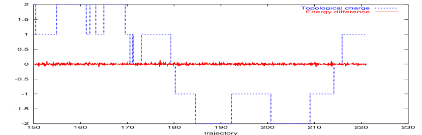
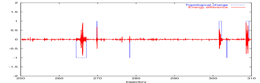
Figure 1: Energy conservation plots for the $4^{4}$ $\beta=5.4$ $\kappa=0.225$, $\mu=0.05$ ensembles, with (top) and without (bottom) chiral projection.

4 NUMERICAL TESTS

We tested the algorithm described in section 2 on $4^{4}$ $\beta=5.4$ lattices with masses $\mu=0.05,0.1,0.2,0.3,0.4$ and $0.5$. Figure 1 plots the topological charge and $dE/d\tau$ ($E$ is the HMC energy) for each molecular dynamics time step for 70 trajectories taken from the $\mu=0.05$ ensembles with and without chiral projection. There are no large spikes in the energy difference, showing that our correction step does indeed conserve energy. Secondly, the chiral projected ensemble, as expected, has more frequent topological charge changes, and a considerably smaller fermionic force when $Q\neq 0$.

$\mu$	$m_{b}$	$<Q^{2}>$	$P_{l}$	$<S_{pf}>$
0.05	0.19	0.016(1)	0.061(21)	0.578(2)
0.1	0.40	0.09(3)	0.064(18)	0.575(2)
0.2	0.89	0.16(3)	0.048(10)	0.568(2)
0.3	1.52	0.24(4)	0.027(9)	0.562(1)
0.4	2.37	0.29(4)	0.032(9)	0.561(1)
0.5	3.56	0.32(10)	0.005(10)	0.554(1)
0.05	0.19	0.01(1)	0.063(6)	0.576(1)
0.1	0.40	0.13(3)	0.071(7)	0.574(1)
0.2	0.89	0.29(4)	0.043(6)	0.569(1)
0.3	1.52	0.34(5)	0.048(8)	0.562(1)
0.4	2.37	.40(5)	0.029(9)	0.559(1)
0.5	3.56	0.45(14)	0.032(13)	0.554(1)

Table 1: The plaquette ($S_{p}g$), Polykov loop ($P_{l}$) and ensemble average of $Q^{2}$ for the $4^{4}$ $\kappa=0.225$ ensembles with (top) and without (bottom) chiral projection.

Table 1 gives the plaquette, Polykov loop, and topological susceptibility for our ensembles. The plaquettes and Polykov loops are in good agreement between the chiral projected and non-chiral projected ensembles; the average values of $Q^{2}$ (proportional to the topological susceptibility) are not, for reasons which we will outline in a later paper [5]. The general behaviour of the plaquette and topological susceptibility are in agreement with our expectations at these large masses (our smallest mass is of the same order of magnitude as the strange quark mass), and the Polykov loop is small, suggesting that our configurations are confined.

5 CONCLUSIONS

We have shown that it is possible to run dynamical simulations using overlap fermions, and that the delta function in the fermionic force can be overcome. The results on our small test configurations are sensible. We hope to begin simulations on $12^{4}$ and similar lattices in the next year.

References

- [1] G. Arnold, N. Cundy, J. van den Eshof, A. Frommer, S. Krieg, T. Lippert, K. Schäfer, Submitted to proceedings of Third International Workshop on Numerical Analysis and Lattice QCD, hep-lat/0311025 .
- [2] N. Cundy, et al., To appear in Comput. Phys. Commun., hep-lat/0405003 .
- [3] S. Krieg, N. Cundy, F. A., J. van der Eschof, T. Lippert, K. Schäfer, these Proceedings, hep-lat/0409030.
- [4] S. Duane, A. Kennedy, B. Pendelton, D. Roweth, Phys. Lett. B195 (1987) 216.
- [5] N. Cundy, A. Frommer, S. Krieg, T. Lippert, nearing completion.
- [6] Z. Fodor, S. Katz, K. K. Szabo, hep-lat/0311010.
- [7] K. K. Szabo, Z. Fodor, S. Katz, these Proceedings, hep-lat/0409070.
- [8] A. Bode, U. M. Heller, R. G. Edwards, R. Narayanan, in: Dubna 1999, Lattice fermions and structure of the vacuum, 1999, pp. 65–68, hep-lat/9912043.