The $F$ model on dynamical quadrangulations

Abstract

The dynamically triangulated random surface (DTRS) approach to Euclidean quantum gravity in two dimensions is considered for the case of the elemental building blocks being quadrangles instead of the usually used triangles. The well-known algorithmic tools for treating dynamical triangulations in a Monte Carlo simulation are adapted to the problem of these dynamical quadrangulations. The thus defined ensemble of 4-valent graphs is appropriate for coupling to it the 6- and 8-vertex models of statistical mechanics. Using a series of extensive Monte Carlo simulations and accompanying finite-size scaling analyses, we investigate the critical behaviour of the 6-vertex $F$ model coupled to the ensemble of dynamical quadrangulations and determine the matter related as well as the graph related critical exponents of the model.

and

1 Introduction

Einstein gravity being perturbatively non-renormalizable as a field theory, constructive approaches towards a quantization of gravity have been an ever more active field of research in the past decades [smolin:03a, ]. The dynamical triangulations model in its Euclidean and Lorentzian versions has proved a successful ansatz for the formulation of such a consistent theory of quantum gravity [ambjorn:book, , ambjorn:00c, ]. Compared to the more fancy methods, such as string theory [witten:99a, ] and non-commutative geometry [connes:00a, ], it is rather more minimalistic in trying to directly model the quantum fluctuations of space-time by a probabilistic sum over an ensemble of discrete, simplicial manifolds [weingartenundco, ]. For the Euclidean case in two dimensions, this ensemble can be defined as the set of all gluings of equilateral triangles to a regular, usually closed surface of fixed topology, while counting each of the possible gluings with equal weight. The resulting random-surface model and its simplicial generalisation to higher dimensions are numerically tractable, for instance by Monte Carlo simulations. Furthermore, for the case of two dimensions the use of matrix models and generating-function techniques led to exact solutions for the cases of pure Euclidean gravity [brezin:78a, , boulatov:86a, ] and the coupling of certain kinds of matter, such as the Ising model [kazakov:86a, , boulatov:87a, , burda, ], to the surfaces. These two-dimensional theories generically exhibit continuous phase transitions on tuning the relevant coupling parameters accordingly and thus allow for taking the intended continuum limit. In the case of matter variables coupled to two-dimensional dynamical triangulations, the critical exponents governing the transitions are conjectured exactly from conformal field theory as functions of the exponents on regular lattices via the so-called KPZ/DDK formula [kpzddk, ]

$$\tilde{\Delta}={\sqrt{1-C+24\Delta}-\sqrt{1-C}\over\sqrt{25-C}-\sqrt{1-C}},$$ (1)

where $\Delta$ is the original scaling weight, $\tilde{\Delta}$ the scaling weight after coupling to gravity and $C$ the central charge. The field-theory ansatz leading to Eq. (1) breaks down for central charges $C>1$, an effect which has been termed the $C=1$ “barrier”, whereas the discrete model of $C>1$ matter coupled to dynamical triangulations stays well defined. This mismatch of descriptions and its driving mechanism is still one of the rather poorly understood aspects of the dynamical triangulations model [david:97a, , ambjorn:00c, , ambjorn:00d, ].

Ice-type or vertex models on regular lattices form one of the most general classes of models of statistical mechanics with discrete symmetry (for reviews see, e.g., Refs. [lieb:domb, , baxter:book, ]). Special cases of this class of models can be mapped onto more well-known problems such as Ising and Potts models or graph colouring problems [baxter:book, ]. For the case of two-dimensional lattices, several of these vertex models can be solved exactly, yielding a very rich and interesting phase diagram including various transition lines as well as critical and multi-critical points [baxter:book, ]. Thus, for two-dimensional vertex models one has the rare combination of a rich structure of phases and an exceptional completeness of the available analytical results. Hence, coupling this class of models to a fluctuating geometry of the dynamical triangulations type is of obvious interest, both as a prototypic model of statistical mechanics subject to annealed connectivity disorder and as a paradigmatic type of matter coupled to two-dimensional Euclidean quantum gravity. Recently, the use of matrix model methods led to a solution of the thermodynamic limit of a special 6-vertex model, the $F$ model, coupled to planar $\phi^{4}$ graphs [zinn, ]. It was found to correspond to a $C=1$ conformal field theory, i.e., it lies on the boundary to the region $C>1$, where the KPZ/DDK solution [kpzddk, ] breaks down. Also, a special slice of the 8-vertex model could be analysed via transformation to a matrix model [kazakov:99a, ]. A generalisation of this result to the general parameter space of the 8-vertex model is currently being attempted [ambjorn:01a, , zinn-justin:03a, ]. However, owed to the method of matrix integrals, these studies neither reveal the behaviour of the matter related observables and the details of the occurring phase transitions nor the fractal properties of the graphs such as, e.g., their Hausdorff dimension. Especially, for the case of the 6-vertex model, which turns out to exhibit a phase transition of the Berezinskii-Kosterlitz-Thouless (BKT) type, quantities related to the staggered, anti-ferroelectric order parameter cannot be easily constructed, such that a detailed numerical analysis of the problem seems valuable. Numerically it is found here that, due to the combined effect of the presence of logarithmic corrections to scaling expected for a $C=1$ theory and the comparative smallness of the effective linear extent of the accessible graph sizes, the leading scaling behaviour is obscured by extremely strong finite-size corrections. Thus, a very careful scaling analysis incorporating the various correction terms has to be performed in order to disentangle the corrections from the asymptotic scaling form.

Since the 6- and 8-vertex models of statistical mechanics are defined on a lattice with four-valent vertices, instead of considering dynamical triangulations or the dual planar, “fat” (i.e., orientable) $\phi^{3}$ graphs, one has to use an ensemble of dynamical quadrangulations or the dual $\phi^{4}$ Feynman diagrams as the geometry to model the coupling of vertex models to quantum gravity. This can be rather easily done within the framework of matrix model methods [brezin:78a, , thooft:99a, ]. For Monte Carlo studies, however, it turns out that the well established simulation techniques for dynamical triangulations [boulatov:86a, , pachner:91a, , ambjorn:94a, ] are quite cumbersome to adapt to the case of four-valent graphs which, therefore, only very scarcely have been considered in the literature [johnston:93a, , baillie:95a, ]. Especially, ergodicity for the selected set of moves has to be ensured and a method of coping with the observed severe critical slowing down of the dynamics, such as an adaption of the “baby-universe surgery” method [ambjorn:94a, , ambjorn:95e, ], has to be devised. The details of these modifications to the simulation scheme will be presented in a separate publication [prep, ].

The rest of this paper is organised as follows. In Sec. 2 we first review the basic properties of vertex models on regular lattices. We shortly discuss the matrix-model solution of the 6-vertex model and elaborate on the necessary conceptual and simulational modifications for considering vertex models on random graphs. Section 3 is devoted to an in-depth investigation of the BKT phase transition of the 6-vertex $F$ model coupled to planar, “fat” $\phi^{4}$ graphs by means of an extensive series of Monte Carlo simulations. In Sec. 4 we present our numerical results for the geometrical properties of the coupled system, such as the string susceptibility exponent and the internal Hausdorff dimension. Finally, Sec. 5 contains our conclusions.

2 Vertex models on random graphs

2.1 Vertex models on regular lattices

An ice-type or vertex model was first proposed by Pauling [pauling, ] as a model for (type I) ice. In this model, the two possible positions of the hydrogen atoms on the bonds of the crystal formed by the oxygens, if symbolised by arrows, lead to six different allowed configurations around a vertex provided that the experimentally observed ice rule is satisfied, stating that each vertex has two incoming and two outgoing arrows, see, e.g., Ref. [baxter:book, ]. While for the original ice model all vertex configurations were counted with equal probability, for the general 6-vertex model vertex energies $\epsilon_{i}$ are introduced, resulting in Boltzmann factors $\omega_{i}=\exp(-\epsilon_{i}/k_{B}T)$, where $T$ denotes temperature and $k_{B}$ is the Boltzmann constant. Some symmetry relations are commonly assumed between the weights $\omega_{i}$; in particular, given the interpretation of the arrows as electrical dipoles, in the absence of an external electric field the partition function should be invariant under a simultaneous reversal of all arrows, leading to the identities $a=\omega_{1}=\omega_{2}$, $b=\omega_{3}=\omega_{4}$ and $c=\omega_{5}=\omega_{6}$. An especially symmetric version of the model assumes $\epsilon_{a}=\epsilon_{b}=1$, $\epsilon_{c}=0$ or $a=b$, $c=1$. This so-called $F$ model [rys:63a, ] turns out to exhibit an anti-ferroelectrically ordered ground state. The square-lattice, zero-field 6-vertex model has been solved exactly in the thermodynamic limit by means of a transfer matrix technique (Bethe ansatz) by Lieb [lieb, ] and Sutherland [sutherland:67a, ]. The analytic structure of the free energy is most conveniently parameterised in terms of the variable [baxter:book, ]

$$\Delta=\frac{a^{2}+b^{2}-c^{2}}{2ab}.$$ (2)

The free energy takes a different analytic form depending on whether $\Delta<-1$, $-1<\Delta<1$ or $\Delta>1$. Thus, phase transitions occur, whenever $|\Delta|=1$. The case $\Delta>1$ corresponds to two symmetry-related ferroelectrically ordered phases termed I and II, $\Delta<-1$ denotes an anti-ferroelectrically ordered phase IV and $-1<\Delta<1$ is attained in the disordered phase III. The latter phase has the peculiarity of having an infinite correlation length throughout, which can be traced back to the fact that it corresponds to a critical surface of the more general 8-vertex model [baxter:book, ]. From Eq. (2) it is obvious that the $F$ model exhibits a phase transition on cooling down from the infinite-temperature point $a=b=c=1$ contained in the disordered phase III to somewhere in the anti-ferroelectrically ordered phase IV. The transitions I $\rightarrow$ III and II $\rightarrow$ III are first-order phase transitions [baxter:book, ]. The transition III $\rightarrow$ IV of the $F$ model, on the other hand, exhibits an essential singularity of the free energy known as the BKT phase transition [kt, ].

While the ferroelectrically ordered phases exhibit an overall polarisation which can be used as an order parameter for the corresponding transition, the anti-ferroelectric order of phase IV is accompanied by a staggered polarisation with respect to a sub-lattice decomposition of the square lattice. That is, when decomposing the square lattice into two new square lattices tilted by $\pi/4$ against the original one, the anti-ferroelectric ground states correspond to a ferroelectric ordering of the vertices of the sub-lattices with opposite signs of the overall polarisation of the sub-lattices. An order parameter for the corresponding transition can be defined by introducing overlap variables $\sigma_{i}$ for each vertex of the lattice such that $\sigma_{i}=v_{i}\ast v_{i}^{0}$, where $v_{i}$ denotes the arrow configuration at vertex $i$, $v_{i}^{0}$ one of the two anti-ferroelectric ground-state configurations and the product “$\ast$” symbolises the overlap given by

$$v\ast v^{\prime}\equiv\sum_{k=1}^{4}A_{k}(v)A_{k}(v^{\prime}),$$ (3)

where $k$ numbers the four edges around each vertex and $A_{k}(v)$ should be $+1$ or $-1$ depending on whether the corresponding arrow of $v$ points out of the vertex or into it [baxter:book, ]. Then, the spontaneous staggered polarisation $P_{0}=\langle\sigma_{i}\rangle/2=\langle\sigma\rangle/2$ vanishes in the disordered phase and approaches unity in the thermodynamic limit for low temperatures in phase IV and can thus be used as an order parameter for the anti-ferroelectric transition.

Vertex models on regular lattices are closely linked with different series of integrable models, which in turn are related to an exhaustive enumeration of certain conformal field theories. In fact, it turns out that the 6-vertex model, being the critical version of the 8-vertex model, includes in suitable generalisations the critical points of all of the well-known two-dimensional lattice models of statistical mechanics, including the Ising and Potts models as the most prominent examples. Especially, the restricted solid-on-solid (RSOS) models [andrews:84a, ], which realise each central charge of the unitary series of minimal models [huse:84a, ], have been shown to asymptotically map onto the 8-vertex model, such that the critical RSOS models correspond to 6-vertex models. Furthermore, an impressive series of models in two dimensions can be mapped onto the Coulomb gas [nienhuis:domb, ]. In these mappings, an intermediate step is always given by models of the solid-on-solid (SOS) type, which again can be related to vertex models [beijeren:77a, ]. Combining these methods, the 6-vertex model can be described as the common element among critical systems in two dimensions [pasquier, ].

2.2 Vertex models on random lattices

Putting a vertex model onto a random four-valent graph such as the quantum gravity $\phi^{4}$ graphs imposes an additional restriction on the class of vertex weights that can be sensibly considered. The ferroelectrically ordered phases I and II of the 6-vertex model and the order parameter describing the corresponding phase transition depend on the existence of a global notion of direction. On a random graph, this notion is maldefined. The only local orientational structure available is that of the vertices and faces of the graph. Thus, for an 8-vertex model coupled to quantum-gravity $\phi^{4}$ random graphs, one has to assume that $a=b$, while the other vertex types can still be distinguished with only a cyclic ordering of the links around each vertex. For the 6-vertex model this leaves only two fundamentally different choices of models to be sensibly considered: the $F$ model with $\epsilon_{a}=\epsilon_{b}=1$, $\epsilon_{c}=0$ and the so-called inverse F (IF) model with $\epsilon_{a}=\epsilon_{b}=-1$, $\epsilon_{c}=0$, which, however, is not of much interest here due to its lack of an ordered phase.

For the square lattice an order parameter for the anti-ferroelectric transition of the $F$ model could be defined by a suitably calculated overlap between the actual state and one of the two anti-ferroelectrically ordered ground states. On a random graph, the corresponding ground states are not so easily found and, moreover, vary between different realisations of the connectivity of the graph. Hence, to define an anti-ferroelectric order parameter for the random graph case, a different and more suitable representation of the vertex model has to be sought. Above, the anti-ferroelectrically ordered state has been described as mutually opposite ferroelectric order on two complementary sub-lattices. A decomposition of the square lattice of this kind corresponds to a bipartition or two-colouring of its sites. Unfortunately, the considered random $\phi^{4}$ graphs are not bipartite in general, preventing an immediate application of this prescription. When interpreting the vertex-model arrows as a discrete vector field on the lattice, the ice rule for the 6-vertex model translates to a zero-divergence condition for this field. We thus transform the vertex model from its interpretation as a field on the links of the original lattice to a representation of the curl of this field on the faces of the lattice or, equivalently, the sites of the dual lattice. Following Stokes’ theorem, this is done by integrating the vertex model arrows around the elementary plaquettes. By convention, plaquettes are traversed counter-clockwise, adding $+1$ for each arrow pointing in the direction of motion and $-1$ otherwise. On the square lattice the resulting “spins” (or “heights”) on the plaquettes can assume the values $0$, $\pm 2$, $\pm 4$. This is demonstrated in Fig. 1. In this way, the 6-vertex model can be transformed to a sort of “spin model” on the dual of the original lattice. Note, however, that one has rather involved restrictions for the “spin” values allowed between neighbouring plaquettes, which would lead to quite cumbersome interaction terms when trying to write down a Hamiltonian.

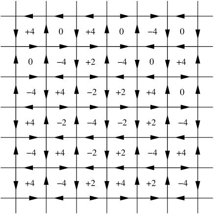
Figure 1: Transformation of the square-lattice 6-vertex model to a “spin” model on the dual lattice. The four links of each plaquette of the lattice are traversed counter-clockwise. The “spin” values written in the centres of the plaquettes are oriented sums of $\pm 1$ around the plaquettes. Thus, the occurring “spin” values are $0,\pm 2,\pm 4$.

In the new representation, the anti-ferroelectrically ordered state of the model again has a sub-lattice structure. However, in contrast to the sub-lattice decomposition of the original representation, now the dual lattice is broken down into “black” and “white” sub-lattices, such that no two plaquettes of the same colour share a link. Then, an order parameter for the anti-ferroelectric transition can be defined as the thermal average of the sum of the plaquette “spins”, e.g., on the “black” plaquettes. Reflecting the construction of the plaquette “spins” in Fig. 1 it is obvious that this definition of the order parameter exactly coincides with the original definition of Sec. 2.1 on the level of configurations. The difference is, however, that the new definition can be easily generalised to the case of arbitrary lattices, as long as their duals are bipartite. This is the case for the planar random $\phi^{4}$ graphs we are considering since any planar quadrangulation is bipartite. Thus, we can introduce a two-colouring of the faces of the graphs. While for the square lattice the numbers of black and white plaquettes are always the same, the black and white faces of the $\phi^{4}$ random graphs not necessarily occur at equal proportions. Thus, one should take the “spins” of both types of faces into account, however “weighted” with the colour of the faces. Therefore, the configurational value of the staggered polarisation of the $F$ model on a planar $\phi^{4}$ random graph ${\mathcal{G}}$ can be defined as $P\equiv\frac{1}{2}\sum_{v\in V({\mathcal{G}}^{\ast})}C_{v}S_{v}$, where ${\mathcal{G}}^{\ast}$ denotes the dual of the graph, i.e.  the quadrangulation, $V({\mathcal{G}}^{\ast})$ the set of vertices of ${\mathcal{G}}^{\ast}$, $C_{v}=\pm 1$ the “colour” of the plaquette of ${\mathcal{G}}$ corresponding to the vertex $v$ of ${\mathcal{G}}^{\ast}$ and $S_{v}$ the plaquette “spin” at $v$. Recalling the construction of the plaquette “spins”, this can also be written in terms of the $\phi^{4}$ graph ${\mathcal{G}}$ as

$$P=\frac{1}{2}\sum_{f\in F({\mathcal{G}})}\sum_{l_{f}\in f}C_{f}A(l_{f}),$$ (4)

where $F({\mathcal{G}})$ denotes the set of faces of ${\mathcal{G}}$, $l_{f}$ the links of face $f$, $C_{f}=\pm 1$ the “colour” of $f$ and $A(l_{f})=\pm 1$ the direction of the vertex-model arrow on link $l_{f}$ with respect to the prescribed anti-clockwise traversal of the faces. The thermal average $\langle P\rangle/2$ is now taken as the order parameter of a possibly occurring anti-ferroelectric phase transition of the $F$ model coupled to planar $\phi^{4}$ random graphs. Note, however, that due to the overall arrow reversal symmetry of the vertex model the expectation value $\langle P\rangle$ will vanish at any temperature for a finite graph. Thus, for finite graphs we consider the modulus $\langle|P|\rangle$ instead, analogous to the usual treatment of the magnetisation of the Ising model.

As mentioned above in the Introduction, a matrix model related to the $F$ model coupled to planar $\phi^{4}$ random graphs could be solved exactly in the thermodynamic limit [zinn, ]. The solution is related to a transformation of the $F$ model to a model of close-packed loops by using “breakups” of the vertices, i.e., prescriptions for connecting incoming and outgoing arrows. The original weights of the 6-vertex model translate into weights for the oriented loops by assigning a phase factor $\exp(i\mu\pi/2)$ to each left turn and a phase factor $\exp(-i\mu\pi/2)$ to each right turn of an oriented loop [baxter:76a, , baxter:book, ]. Here, the coupling $\mu$ is related to the weights of the $F$ model as

$$a/c=b/c=[2\cos(\pi\mu)]^{-1}.$$ (5)

On the square lattice the phase factors around each loop always multiply up to a total of $\exp(\pm i\mu 2\pi)$ due to the absence of curvature. On a random graph, however, a loop $l$ in general receives a non-trivial weight $\exp[i\mu\Gamma(l)]$ with $\Gamma(l)$ denoting the integral of the geodesic curvature along the curve $l$, i.e.,

$$\Gamma(l)=\frac{\pi}{2}\left(\mbox{\# left turns}-\mbox{\# right turns}\right).$$ (6)

This loop expansion is related to the well-known loop representation of the O($n$) model of Ref. [domany:81a, ]. There, on a regular lattice, due to the absence of curvature all loops receive the same constant fugacity $n=2\exp(\pm i\mu 2\pi)$, leading to the critical O($n$) model. On the considered random graphs this picture only remains valid for the limiting case $\mu=0$, where the curvature dependence cancels. Thus, the $\mu=0$ point of the $F$ model on random planar $\phi^{4}$ graphs is equivalent to the critical O($2$) loop model [kostov:89b, , dalley:92a, , zinn, ] and thus, by universality, the critical $XY$ model. Note that this corresponds to the same critical point $a/c=b/c=1/2$ as on the regular square lattice, which is natural since the symmetry breaking is induced by the choice of the vertex weights. By means of the mentioned matrix model techniques it is found that the $F$ model coupled to planar, “fat” $\phi^{4}$ graphs has a critical point for each value of the coupling $\mu$ (corresponding to the disordered phase III), in agreement with the behaviour on the square lattice. Exploring the vicinity of this critical point, it is found that the string susceptibility exponent $\gamma_{s}=0$ for all $\mu$, leading to only logarithmic divergences of the free energy [zinn, ]. This behaviour is indeed expected from the $C\rightarrow 1$ limit of the KPZ/DDK prediction Eq. (1). Thus, the general phase structure of the $F$ model coupled to planar random $\phi^{4}$ graphs in the grand-canonical ensemble of a varying number of vertices has been found in Ref. [zinn, ]. The existence of a BKT type phase transition at $\mu=0$ was obvious beforehand from the equivalence to the O(2) loop model at this point. Details of the behaviour of matter-related observables close to the critical point, such as the scaling of the staggered anti-ferroelectric polarisability, however, could naturally not be extracted from the matrix model ansatz.

3 The anti-ferroelectric phase transition

The critical point of the $F$ model on the square lattice provided the first example of an infinite-order phase transition of the BKT type. By virtue of the loop expansion sketched above, this behaviour is expected to persist as the model is coupled to a random lattice. In the vicinity of a phase transition of this type, the usual thermal and finite-size scaling (FSS) relations are profoundly changed. Using an elaborate set of simulational techniques specially tailored for simulations of this model, we present a detailed scaling analysis of its thermal properties. As a guideline for the rather involved analysis we used our newly performed set of loop-cluster update simulations of the square-lattice $F$ model [weigel:05a, ], which is computationally less demanding such that much larger system sizes could be investigated. For a general discussion of scaling and FSS at an infinite-order phase transition of the BKT type [kt, ], we refer the reader to this study and references found therein [weigel:05a, ]. Due to the nature of the occurring singularities the main strengths of FSS are found not to apply to the BKT phase transition, and the focus of numerical analyses of the $XY$ and related models has been on thermal scaling, see, e.g., Ref. [gupta, ]. In addition, renormalization group analyses predict logarithmic corrections to the leading scaling behaviour [amit, ], as expected for a $C=1$ theory, which have been found exceptionally hard to reproduce numerically due to the presence of higher order corrections of comparable magnitude [wj:97b, ]. Comparing the phase transitions in the two-dimensional planar and the six-vertex $F$ models, one should keep in mind that due to the dual relation of both models, the rôles of high- and low-temperature phases are exchanged in that the $F$ model has a critical low-temperature phase, whereas the high-temperature phase is massless in the $XY$ model. In contrast to the $XY$ model, the low-temperature phase of the $F$ model exhibits a non-vanishing order parameter, given by the spontaneous polarisation of Eq. (4), such that, although the critical points of both models are equivalent, the magnetisation of the planar model does not correspond to the polarisation of the $F$ model [weigel:05a, ].

3.1 Simulation techniques

For Monte Carlo simulations of two-dimensional combinatorial dynamical triangulations or the dual regular $\phi^{3}$ graphs, an ergodic set of updates for simulations of a fixed number of polygons or graph vertices (canonical ensemble) is given by the so-called Pachner moves [gross:92a, ]. An adaption of the link-flip move for canonical simulations of triangulations to the case of quadrangulations has been proposed in Refs. [johnston:93a, , baillie:95a, ]. By the construction of counter-examples it can be shown that the link-flip moves of Refs. [johnston:93a, , baillie:95a, ] do not in general constitute an ergodic dynamics for canonical simulations of dynamical quadrangulations. Introducing a second type of link-flip moves, we construct an algorithm for canonical simulations of dynamical quadrangulations, which does not show any signs of ergodicity breaking [weigel:02b, , doktor, , prep, ]. A scaling analysis of the thus constructed dynamics reveals that its performance — as expected from a local algorithm — is limited by the effect of critical slowing down. To alleviate this problem, we adapt the non-local “baby-universe surgery” method proposed in Ref. [ambjorn:94a, ] for triangulations to the case of quadrangulations and investigate its dynamical properties by means of a scaling analysis [doktor, , prep, ]. For the vertex model part, we also employ a non-local, cluster algorithm known as “loop-cluster algorithm”, which is known to drastically reduce autocorrelation times for vertex models on the square lattice [evertz:loop, ]. For the application of this simulation scheme to random-lattice models, certain modifications are necessary. The mentioned algorithmic developments for the graph and the vertex model part as well as the technical details of the necessary simulational set-up will be discussed in a separate publication [prep, ].

For the FSS study to be presented below, we simulated a series of spherical $\phi^{4}$ graphs of sizes ranging from $N_{2}=256$ up to $N_{2}=65\,536$ vertices. The simulations where performed at several computing facilities using about 100 000 hours of CPU time in total.

3.2 Scaling analysis

We assume a parameterisation of the $F$ model coupling parameters which involves a temperature variable and thus sticks more closely to the language of statistical mechanics than to that of field theory. It hence differs from the parameterisation (5) used in the context of the matrix model solution, which only covers the critical disordered phase of the $F$ model. Choosing the vertex energies as $\epsilon_{a}=\epsilon_{b}=1$, we have $a=b=e^{-\beta}$, $c=1$, where $\beta=1/k_{B}T$, such that the BKT point occurs for $\beta_{c}=\ln 2$, both for the square-lattice model and, conjectured by the matrix model solution discussed in Sec. 2.2, for the $F$ model coupled to planar $\phi^{4}$ random graphs.

3.2.1 The specific heat

The specific heat $C_{v}$ of the $F$ model coupled to planar $\phi^{4}$ random graphs exhibits a broad peak of around $C_{v}\approx 0.45$, shifted away from the critical point into the low-temperature phase to a centre of $\beta\approx 1.0$. The peak does not depend on the lattice size up to very small finite-size corrections, i.e., no FSS is observed. The expected essential, non-divergent singularity [lieb:domb, , weigel:05a, ] cannot in general be resolved, since it is covered by the presence of non-singular background terms. This non-scaling behaviour of the specific heat is commonly considered as a first good indicator for the presence of an infinite-order phase transition [barber:domb, ].

3.2.2 Location of the critical point

The critical coupling can be determined from the scaling of the shifts of suitably defined pseudo-critical couplings on finite graphs, see Ref. [weigel:05a, ]. Here, we use the locations $\beta_{\chi}$ of the maxima of the staggered anti-ferroelectric polarisability, defined from the generalised polarisation of Eq. (4). In terms of the inverse temperature $\beta$ to first order one has at a BKT transition [weigel:05a, ],

$$\beta_{\chi}(N_{2})=\beta_{c}+A_{\beta}(\ln N_{2})^{-1/\rho},$$ (7)

where $N_{2}$ is the size of the graphs and $\rho=1/2$ for the regular $XY$ and $F$ models barber:domb , baxter:book . For the determination of the peak positions we make use of the temperature-reweighting technique [ferrenberg, ]. Note that the quoted errors do not cover the potential bias induced by the reweighting procedure. We performed simulations for graph sizes between $N_{2}=256$ and $N_{2}=25\,000$ sites, taking some $10^{6}$ measurements after the systems had been equilibrated. Measurements were taken after every tenth sweep of the combined link-flip and “baby-universe surgery” dynamics, using “regular” graphs without self-energy and tadpole insertions [prep, ]. All statistical errors were determined by a combined binning/jackknife technique, cf. Ref. [efron, ].

Comparing the estimated peak locations to the corresponding results for the square-lattice model [weigel:05a, ] one notes that the accessible part of the scaling regime is strongly shifted towards lower temperatures, being rather far away from the conjectured critical coupling $\beta_{c}=\ln 2\approx 0.693$, cf. the “regular ensemble” data of Fig. 2 below. We start with fits of the simple form Eq. (7) without including any correction terms. Additionally, we assume $\rho=1/2$ here as in the square-lattice case, which has to be justified a posteriori by the thermal scaling analysis. Within this scheme, the influence of correction terms is taken into account by successively omitting lattice sizes from the small-$N_{2}$ side. Due to the strong corrections present, however, no fits with satisfactory fit quality can be found in this way such that it appears mandatory to include correction terms. Since the exact form of the present scaling corrections is not known, an effective description has to be employed. One possible ansatz is to relax the constraint $\rho=1/2$, introducing $\tilde{\rho}\neq\rho$ as an additional fit parameter. Even for this type of fit, acceptable fit qualities can only be attained by dropping many of the smaller graph sizes, thus strongly increasing the uncertainty in the estimated parameters. Additionally, we find that the fit results for small minimum included graph sizes $N_{2,\mathrm{min}}$ partly depend on the choice of the starting values for the fit parameters, i.e., that the fit routine gets stuck in local minima of the $\chi^{2}$ distribution. For $N_{2,\mathrm{min}}=4096$ we arrive at an estimate $\beta_{c}=0.83(58)$, $A_{\beta}=1.7(62)$, and $1/\tilde{\rho}=1.0(31)$ with a quality of $Q=0.69$. Statistically, this is in agreement with the expected value $\beta_{c}=\ln 2\approx 0.693$ for the critical coupling, but due to the large statistical error the estimate is of limited significance. The result for the exponent $\tilde{\rho}$ cannot be taken as a serious estimate for $\rho$, since it incorporates corrections effectively.

Table 1: Parameter results of linear fits of the form (8) to the simulation data for the peak locations of the staggered polarisability. Values of parameters held fixed are indicated by square brackets.

$N_{2,\mathrm{min}}$	$\beta_{c}$		$A_{\beta}$		$B_{\beta}$		$C_{\beta}$	$Q$
256	0.	8999(71)	17.	4(11)	$-69$.	4(47)	[0]	0.	02
512	0.	876(13)	21.	9(22)	$-92$.	0(108)	[0]	0.	08
1024	0.	817(24)	33.	7(46)	$-155$.	3(243)	[0]	0.	72
256	0.	779(39)	55.	4(122)	$-424$.	9(1140)	918(294)	0.	32
512	0.	693(75)	87.	0(263)	$-748$.	1(2647)	1838(741)	0.	39

For the square-lattice case, from the exact solution the leading corrections to the form (7) with $\rho=1/2$ could be expressed as a power series in $1/\ln N_{2}$ weigel:05a ,

$$\beta_{\chi}(N_{2})=\beta_{c}+A_{\beta}(\ln N_{2})^{-2}+B_{\beta}(\ln N_{2})^{-3}+C_{\beta}(\ln N_{2})^{-4},$$ (8)

hence we consider this form for the random graph data here as well. As can be seen from the collection of fit parameters in Table 1, this form provides a good description of the data, although some of the statistical errors of the fit parameters become very large. Neglecting the second correction first, i.e., holding $C_{\beta}=0$ fixed, the results are stable on successively omitting data points from the small-$N_{2}$ side, and the resulting estimates for the transition temperature are slowly drifting towards the asymptotic value $\beta_{c}=\ln 2=0.693\ldots$. Nevertheless, the result for, e.g., $N_{2,\mathrm{min}}=1024$, $\beta_{c}=0.817(24)$ is still far from being compatible with the asymptotic result in terms of the statistical error. Including the fourth-order term of (8), on the other hand, further reduces the estimates for $\beta_{c}$ to the extent of being compatible with $\beta_{c}=\ln 2$, however at the price of largely increased statistical errors. For $N_{2,\mathrm{min}}>512$, the fits get very unstable, such that we quote as our final result from this approach $\beta_{c}=0.693(75)$ for $N_{2,\mathrm{min}}=512$. If we finally fix $\beta_{c}$ at its asymptotic value, for $C_{\beta}=0$ we reach a fit quality of $Q=0.01$ only at $N_{2,\mathrm{min}}=2048$, while with variable $C_{\beta}$, $Q=0.52$ is reached already at $N_{2,\mathrm{min}}=512$. This clearly shows that both correction terms are necessary for resolving the scaling corrections, but the accuracy of the present data is only marginally sufficient to do so. It should be noted that also the other types of fits presented here still yield good quality-of-fits when fixing the parameter $\beta_{c}$ at $\ln 2$. For example, a fit of the form (7) with variable exponent $\tilde{\rho}$ to the data with $N_{2,\mathrm{min}}=2048$ gives $A_{\beta}=1.071(81)$, $1/\tilde{\rho}=0.541(35)$, and $Q=0.84$.

3.2.3 Universality of the critical coupling

One might be tempted to suspect that the observed rather large deviations of the finite-size positions of the polarisability maxima from the expected value $\beta_{c}=\ln 2\approx 0.693$ are due to the fact that we use graphs of the regular ensemble, i.e. those without self-energy and tadpole insertions, whereas the matrix model calculations of Ref. [zinn, ] naturally concern graphs of the unrestricted singular ensemble. Indeed, quite generally one does not expect the critical coupling of a model to be universal. In particular, for the Ising model coupled to dynamical polygonifications or the dual graphs, the location of the observed transition does depend on whether one considers spins located on the vertices of triangulations, quadrangulations, $\phi^{3}$ or $\phi^{4}$ graphs [boulatov:87a, , johnston:93a, , baillie:95a, ]. Additionally, depending on the considered ensemble of graphs with respect to the inclusion or exclusion of certain types of singular contributions, one arrives at different values for the critical coupling [boulatov:87a, , jurkiewicz:88a, , burda, , schneider:99a, ]. However, the situation is quite different for the case of the $F$ model coupled to random lattices. As has been mentioned above in Sec. 2.2, in the matrix model description of the problem, the matrix potential becomes equivalent to that of the O($2$) model in the limit $\mu=0$ [zinn, ], which corresponds to the choice $a/c=b/c=1/2$ or $\beta_{c}=\ln 2$. Thus, renormalizing the matrix model to remove some or all of the singular graph contributions does not change the location of the BKT point.

We have not performed extensive simulations of graphs of the “singular” ensemble including self-energy and tadpole insertions to demonstrate this behaviour numerically. This is due to the fact that simulations for graphs of the singular ensemble are by orders of magnitude less efficient for the considered graph sizes than simulations of the other graph ensembles due to details of the implementation of the simulation scheme, cf. Ref. [prep, ]. Nevertheless, we carried out some simulations for smaller graph sizes and analysed the FSS of the peak locations of the staggered polarisability just as for the case of “regular” graphs. The corresponding FSS data are shown in Fig. 2 together with the results for regular graphs. Using Eq. (8) with $C_{\beta}=0$, a fit to the data including all five points from $N_{2}=128$ to $N_{2}=2048$ yields the estimate $\beta_{c}=1.01(11)$, $Q=0.92$, letting $C_{\beta}$ vary gives $\beta_{c}=0.83(69)$, $Q=0.76$, which is in principle in agreement with $\beta_{c}=\ln 2$, although very inaccurate. Note that from Fig. 2 the finite-size corrections for the singular graph case are much larger than those for the regular graph model. This is in contrast to previous observations for the case of the Potts model coupled to random triangulations [ambjorn:95a, ] and the resulting common belief that the inclusion of singular graph contributions generically reduces FSS corrections.

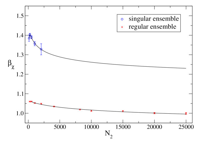
Figure 2: Finite-size approach of the peak locations of the staggered polarisability of the $F$ model on $\phi^{4}$ random graphs with (“singular ensemble”) and without (“regular ensemble”) tadpole and self-energy insertions. The solid lines show fits of the functional form (8) to the data.

As has been mentioned in the Introduction, the reason for the observed very slow approach to the expected asymptotic behaviour lies in the double effect of the presence of logarithmic corrections to scaling and the small effective linear extent of the highly fractal lattices. In principle it should be possible to resolve the resulting scaling corrections by including higher-order correction terms in the fit ansätze. However, it must be admitted that, refraining from any artificial “good-will” tinkering with the fit parameters, the accuracy of the present data is not sufficient for reliable many-parameter, possibly non-linear fits. The strength of this combined effect is nicely demonstrated numerically by the fact that the fits to the FSS of the polarisability peak locations with $\beta_{c}$ fixed to its true value $\beta_{c}=\ln 2$ come as close as $\beta_{\chi}(N_{2})=0.7$ to the critical value only for graph sizes $N_{2}\approx 10^{100}$ for the form (8) with variable $C_{\beta}$ or even $N_{2}\approx 10^{5000}$ for the form (7) with variable exponent $\tilde{\rho}$. Instead of figuring out more elaborate fits, we try to disentangle the two correction effects by a comparison to the square-lattice model, where only the logarithmic corrections are present, but the considered lattices are not fractal [weigel:05a, ]. For this purpose, we plot in Fig. 3 the polarisability peak locations as a function of the root mean square extent of the considered lattices defined as

$$\langle r^{2}\rangle_{N_{2}}^{1/2}=\left\langle\frac{\sum_{r=0}^{r_{\mathrm{max}}}r^{2}G_{11}(r)}{\sum_{r=0}^{r_{\mathrm{max}}}G_{11}(r)}\right\rangle_{N_{2}}^{1/2},$$ (9)

which is the relevant measure for the linear extent of the graphs. Here, we take the geometrical two-point function $G_{11}(r)$ as the number of graph vertices with a geodesic link distance $r$ from a randomly chosen reference point $p_{0}$. The root mean square extents $\langle r^{2}\rangle^{1/2}$ are related to the number of graph vertices according to $\langle r^{2}\rangle\sim N_{2}^{2/d_{h}}$, which defines the internal Hausdorff dimension $d_{h}$. Due to the fractal structure of the random graphs, largely differing values of the root mean square extent $\langle r^{2}\rangle^{1/2}$ are found for them in comparison to square lattices with the same number of vertices $N_{2}$. For the latter data (which are basically exact) this scaling ansatz without inclusion of any correction terms yields $d_{h}=2.000(20)$, where the error reflects discretisation effects for small lattices. For the case of $\phi^{4}$ random graphs the fit yields $d_{h}=3.336(11)$. Note, however, that the result for $d_{h}$ is slowly increasing as more and more of the small-$N_{2}$ lattices are excluded and we expect the true value of the Hausdorff dimension to be somewhat larger, see Refs. [kawamoto:92a, , ambjorn:97b, , ambjorn:98d, ] and Sec. 4 below. Hence, in order to obtain results for the $F$ model at comparable linear extents of the square and random lattices, one has to consider rather small volumes for the square-lattice case. For the comparison we use $L\times L$ square lattices, where the edge lengths $L$ were chosen such that the resulting root mean square extent comes as close as possible to the $\langle r^{2}\rangle^{1/2}$ values for the corresponding $\phi^{4}$ random graphs. The volumes of the $\phi^{4}$ random graphs were chosen between $N_{2}=256$ and $N_{2}=8192$, increasing in powers of two.

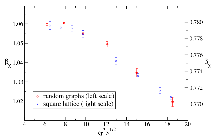
Figure 3: Collapse of the FSS approach of the scaling of the peak locations of the staggered anti-ferroelectric polarisability of the $F$ model on random $\phi^{4}$ graphs (left scale) and on the square lattice (right scale). The data for the square-lattice model are taken from a set of simulations presented in Ref. [weigel:05a, ].

In Fig. 3 we present a comparison of the FSS approach of the peak locations of the polarisability for the $\phi^{4}$ graph and square-lattice [weigel:05a, ] models plotted as a function of the linear extent $\langle r^{2}\rangle^{1/2}$ of the lattices. Here, the abscissae of the plot have been scaled such as to account for the difference in the overall correction amplitude, but assuming the same value $\ln 2$ for the offset. From the two simulation points near ${\langle r^{2}\rangle}^{1/2}\approx 10$ we find the ratio of the correction amplitudes as

$$A_{\beta}=\frac{\beta_{\chi}^{\mathrm{rl}}(N_{2}=1024)-\ln 2}{\beta_{\chi}^{\mathrm{sl}}(N_{2}=324)-\ln 2}\approx 4.23,$$ (10)

where $\beta_{\chi}^{\mathrm{rl}}$ denotes the peak position for the random $\phi^{4}$ graph model and $\beta_{\chi}^{\mathrm{sl}}$ the value for the square lattice. The thus achieved collapse of the FSS data is obvious from Fig. 3. Consequently, we come to the clear conclusion that the larger deviations of the peak locations for random graphs are simply due to an about four times larger overall amplitude of the correction terms as compared to the square-lattice model, the details of the FSS approach being otherwise surprisingly similar between the two considered lattice types. Especially, the fact that for the $\phi^{4}$ graph case the asymptotic value $\beta_{c}=\ln 2$ cannot be clearly resolved by the considered fits to the data is an obvious consequence of the comparative smallness of the accessible lattice sizes in terms of their effective linear extents $\langle r^{2}\rangle^{1/2}$. To underline this finding, we performed fits of the simple form (7) to the data for both types of lattices (there are not enough data points for fits with correction terms), including sizes starting from the points near $\langle r^{2}\rangle^{1/2}\approx 10$, which result in estimates $\beta_{c}=0.7554(18)$ for the square lattice and $\beta_{c}=0.9416(89)$ for the random graphs. In terms of the quoted statistical errors these are obviously both far away from the asymptotic result. The deviation from $\beta_{c}=\ln 2$ is, however, just about four times larger for the random graph case than for the square-lattice model, in agreement with the previous discussion of the scaling collapse of Fig. 3.

3.2.4 Critical energy and specific heat

As an aside, we note that for the largest $\phi^{4}$ random graphs we have simulated, i.e., for $N_{2}=65\,536$, at $\beta=\beta_{c}=\ln 2$ we find the following values of the internal energy and specific heat per site,

$$U(\beta=\ln 2)=0.333355(11),\;\;\;C_{v}(\beta=\ln 2)=0.2137(12).$$ (11)

Comparing these results to the values found analytically for the square-lattice $F$ model [lieb:domb, ], $U(\beta_{c})=1/3$, $C_{v}(\beta_{c})=28(\ln 2)^{2}/45\approx 0.2989$, we see that $U(\beta=\ln 2)$ is very close to the value found for the square lattice, whereas $C_{v}(\beta=\ln 2)$ is far away from the square-lattice result. On the basis of these findings, we conjecture that the critical value of the internal energy of the $F$ model is not affected by the coupling to random graphs, while the critical specific heat is. Thus, as one would expect, the critical distribution of vertex energies naturally changes its shape on moving from the square-lattice to the random graph model, but, curiously, its mean is not shifted by this procedure. Interestingly, this situation seems to be specific to the critical point $\beta_{c}=\ln 2$ common to both models, where the two curves cross. For other inverse temperatures the square-lattice and random graph energies diverge, see Fig. 4. This probably indicates the presence of an additional symmetry at criticality.

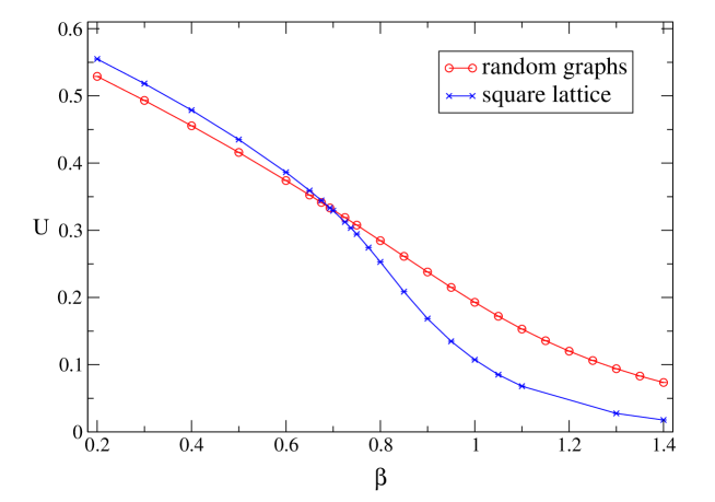
Figure 4: Temperature dependence of the internal energy $U$ of the square-lattice and random $\phi^{4}$ graph $F$ models. Simulations have been performed for a $N_{2}=46^{2}=2116$ square lattice and random graphs with $N_{2}=2048$ sites.

3.2.5 FSS of the polarisability

On coupling the vertex model to quantum gravity we expect a renormalization of the critical exponents as prescribed by the KPZ/DDK formula (1). In Ref. [kpzddk, ] KPZ/DDK focus on conformal minimal models with $C<1$ coupled to the Liouville field, but their work should also marginally apply to the limiting case $C=1$ of the model considered here. The KPZ/DDK formula prescribes a dressing of the conformal weights on coupling a matter system to the fluctuating background. To find the usual critical exponents from the weights, one assumes that the well-known scaling relations stay valid and thus arrives at

$$\begin{array}[]{l}\displaystyle\alpha=\frac{1-2\Delta_{\epsilon}}{1-\Delta_{\epsilon}},\;\;\;\beta=\frac{\Delta_{P}}{1-\Delta_{\epsilon}},\;\;\;\gamma=\frac{1-2\Delta_{P}}{1-\Delta_{\epsilon}},\\ \displaystyle d_{h}\nu=\frac{1}{1-\Delta_{\epsilon}},\;\;\;2-\eta=(1-2\Delta_{P})d_{h}.\end{array}$$ (12)

Here, $\Delta_{\epsilon}$ denotes the weight of the energy operator and $\Delta_{P}$ symbolises the weight of the scaling operator corresponding to the spontaneous staggered polarisation $P_{0}$, which here takes on the rôle of the magnetisation operator $\sigma$ of magnetic models. For the special case of the infinite-order phase transition considered here, the usual exponents written above are not well-defined in the sense of describing power-law singularities. However, the corresponding FSS exponents, i.e., $\beta/d_{h}\nu=\Delta_{P}$ and $\gamma/d_{h}\nu=1-2\Delta_{P}$, still have a well-defined meaning. From the exponent $\beta/d_{h}\nu=1/4$ for the square-lattice $F$ model (with $d_{h}=d=2$) [weigel:05a, ], we find $\Delta_{P}=1/4$. Note that this weight is different from the weight $\Delta_{\sigma}=1/16$ found for the magnetisation of the critical $XY$ model in two dimensions, see e.g. Ref. [henkel:book, ]. For central charge $C=1$ from Eq. (1) one arrives at $\tilde{\Delta}_{P}=1/2$ and the dressed critical exponents become $\beta/d_{h}\nu=\tilde{\Delta}_{P}=1/2$ and $\gamma/d_{h}\nu=1-2\tilde{\Delta}_{P}=0$, implying a merely logarithmic singularity of the staggered polarisability for dynamical graphs.

For a numerical check of these conjectured exponents, there are the two principal possibilities of considering the FSS of the staggered polarisability at its maxima for the finite graphs or at the fixed asymptotic transition coupling $\beta_{c}=\ln 2$. While in the asymptotic regime both approaches are expected to lead to identical results, this is not at all obvious in the presence of large, not completely controlled correction effects for the accessible graph sizes. In both cases, by analogy to the situation on the square lattice [weigel:05a, ] we start from an FSS form including a leading effective correction term, namely,

$$\chi(N_{2})=A_{\chi}N_{2}^{\gamma/d_{h}\nu}(\ln N_{2})^{\omega_{\chi}},$$ (13)

where $\chi(N_{2})$ is taken to be either the peak value as a function of $\beta$ or the value at $\beta=\beta_{c}=\ln 2$. We consider the peak value case first, taking the simulation results for the graph sizes $N_{2}=256,\ldots,25\,000$. Omitting the correction term, i.e., forcing $\omega_{\chi}=0$, and trying to control the effect of corrections to scaling by successively omitting data points from the small-$N_{2}$ side, results in quite poor fits with an exponent estimate $\gamma/d_{h}\nu\approx 0.7$ steadily decreasing with increasing lower cut-off $N_{2,\mathrm{min}}$. Allowing the effective correction exponent $\omega_{\chi}$ to vary, the resulting leading exponent estimate $\gamma/d_{h}\nu$ is considerably reduced, still showing a tendency to decline as $N_{2,\mathrm{min}}$ is increased, cf. Table 2(a). However, the fit quality is still not very good and the resulting exponent estimate for, e.g., $N_{2,\mathrm{min}}=2048$, $\gamma/d_{h}\nu=0.301(79)$ is not consistent in terms of the statistical error with the purely logarithmic singularity expected from the KPZ/DDK prediction. These results in principle might be improved by including corrections of the form $1/(\ln N_{2})^{n}$, $n=1,2,\ldots$ as in the square-lattice case weigel:05a , but the present data are not precise enough to reliably fit these terms.

Table 2: Results of fits of the functional form (13) to the simulation data for the staggered polarisability. (a) Fits to the data at the polarisability peak locations. (b) Fits to the data at the asymptotic critical coupling $\beta=\beta_{c}=\ln 2$.

(a)	$N_{2,\mathrm{min}}$ $A_{\chi}$ $\gamma/d_{h}\nu$ $\omega_{\chi}$ $Q$ 256 0. 1975(97) 0. 4749(81) 1. 698(55) 0. 00 512 0. 116(14) 0. 406(16) 2. 22(12) 0. 00 1024 0. 039(12) 0. 281(37) 3. 24(30) 0. 24 2048 0. 047(37) 0. 301(79) 3. 07(68) 0. 16
(b)	$N_{2,\mathrm{min}}$ $A_{\chi}$ $\gamma/d_{h}\nu$ $\omega_{\chi}$ $Q$ 256 0. 491(19) 0. 0194(55) 2. 117(40) 0. 66 512 0. 543(42) 0. 0304(91) 2. 026(72) 0. 91 1024 0. 569(75) 0. 035(14) 1. 98(12) 0. 85

For the data at fixed coupling $\beta_{c}=\ln 2$, simulations up to slightly larger graph sizes could be performed since no reweighting analysis is necessary there. Hence, results are available for graph sizes between $N_{2}=256$ and $N_{2}=32\,768$ sites, increasing by powers of two. For the constrained fits of the functional form (13) with $\omega_{\chi}=0$ we do not find a quality-of-fit of at least $10^{-2}$ for $N_{2,\mathrm{min}}$ up to $4096$ and thus do not consider this form further. The parameters of fits including the logarithmic term are collected in Table 2(b), revealing that the functional form including a logarithmic correction fits the data rather well already for quite small values of $N_{2,\mathrm{min}}$, leading to exponent estimates $\gamma/d_{h}\nu$ compatible with the conjecture $\gamma/d_{h}\nu=0$ in terms of the quoted statistical errors. In fact, if we assume a purely logarithmic increase of $\chi(N_{2})$, i.e., if we fix $\gamma/d_{h}\nu=0$, the data yield good-quality fits for $N_{2,\mathrm{min}}\gtrsim 512$; for $N_{2,\mathrm{min}}=2048$ the parameters of this purely logarithmic fit are $A_{\chi}=0.3960(96)$, $\omega_{\chi}=2.295(11)$, with $Q=0.39$.

The simulation data at $\beta=\ln 2$ together with this last fit are shown in Fig. 5. Note that for the peak-height data discussed before, such a purely logarithmic fit is not possible with acceptable values of $Q$. To enable a somewhat better judgement of the observed discrepancy between the scaling at the peak maxima and at $\beta_{c}=\ln 2$, we considered the same two lines for the square-lattice model [weigel:05a, ], using a range of lattice sizes comparable to that of the random graph case in terms of the effective linear extents as it has been discussed in Sec. 3.2.3. Fitting the functional form (13) with variable $\omega_{\chi}$ to these two square-lattice data sets, we find $\gamma/d_{h}\nu=0.475(46)$ for the scaling at $\beta=\ln 2$ also considered above, but an estimate of $\gamma/d_{h}\nu=0.598(36)$ from the scaling of the peak values of $\chi$. Thus, also for the square-lattice model, the scaling of the peak values yields an exponent estimate lying off the expected result ($\gamma/d_{h}\nu=1/2$ in this case), while fits at the critical coupling are in good agreement with the expectations. This is in agreement with the general observation of enhanced correction amplitudes of the random graph model compared to the square-lattice case reported in Sec. 3.2.3.

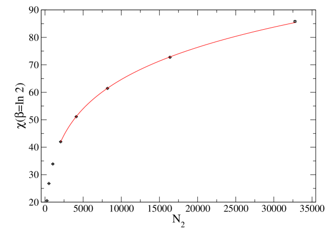
Figure 5: Finite-size simulation data of the polarisability of the $F$ model on random $\phi^{4}$ graphs at the asymptotic critical coupling $\beta_{c}=\ln 2$. The solid curve shows a fit of the form (13) to the data, where $\gamma/d_{h}\nu=0$ was kept fixed.

3.2.6 FSS of the spontaneous polarisation

For the scaling of the spontaneous polarisation the situation is found to be quite similar to the above discussed case of the polarisability. We assume the same leading FSS form as in the square-lattice case [weigel:05a, ], i.e.,

$$P_{0}(N_{2})=A_{P_{0}}N_{2}^{-\beta/d_{h}\nu}(\ln N_{2})^{\omega_{P_{0}}},$$ (14)

where, again, $P_{0}(N_{2})$ is taken to be either the value at the peak position of the polarisability or, alternatively, the result at the asymptotic critical coupling $\beta_{c}=\ln 2$. Fits without the logarithmic correction term ($\omega_{P_{0}}=0$) show unacceptable quality throughout the whole region of choices of the cut-off $N_{2,\mathrm{min}}$ and for both FSS series. For the polarisation at the peak locations of the polarisability, even fits including the logarithmic correction term of Eq. (14) show very poor fit quality and estimates for $\beta/d_{h}\nu$ which are clearly too small compared to the KPZ/DDK prediction $\beta/d_{h}\nu=1/2$ in terms of their statistical errors. We attribute this to the generally more pronounced corrections for the values at the polarisability peak locations already noted above. In addition, however, the non-divergent behaviour of the polarisation makes it even harder to resolve the correction terms properly, and the possible presence of systematic reweighting errors (bias) has much more severe effects here due to the higher statistical accuracy of the polarisation estimate. Again, the analogous analysis of the FSS of the square-lattice model reveals a similar behaviour for comparable graph sizes in terms of the linear extent, however with the size of the deviations from the expected result being much smaller.

Table 3: Parameters resulting from fits of the form (14) to the finite-graph spontaneous polarisation at the infinite-volume critical coupling $\beta_{c}=\ln 2$.

$N_{2,\mathrm{min}}$	$A_{P_{0}}$		$\beta/d_{h}\nu$		$\omega_{P_{0}}$		$Q$
256	1.	583(35)	0.	4633(30)	0.	726(22)	0.	74
512	1.	658(68)	0.	4581(50)	0.	684(39)	0.	91
1024	1.	58(11)	0.	4633(79)	0.	728(64)	0.	98
2048	1.	48(23)	0.	469(15)	0.	779(134)	1.	00

Table 3 shows the parameters resulting from least-squares fits of Eq. (14) to the simulation data at the fixed coupling $\beta=\beta_{c}=\ln 2$. The overall quality of the fits is much better than for the data at the polarisability peak locations discussed before. This is at least partially due to the fact that for the results at fixed coupling no bias effects induced by a reweighting procedure are present. We do not observe a clear overall drift of the exponent estimate $\beta/d_{h}\nu$ resulting from the fits as a function of the cut-off $N_{2,\mathrm{min}}$ and the quality-of-fit is found to be exceptionally high already for small values of $N_{2,\mathrm{min}}$. The result for $N_{2,\mathrm{min}}=2048$ is consistent with the KPZ/DDK conjecture $\beta/d_{h}\nu=1/2$ within about two times the quoted standard deviation. We note that the estimated correction exponents $\omega_{\chi}$ and $\omega_{p_{0}}$ are found to be clearly different from each other. In fact, from the exact solution of the square-lattice model, both exponents are found to be different even asymptotically [weigel:05a, ]. In addition, both exponents effectively capture the presence of sub-leading corrections for the two observables, leading to the occurrence of further differences.

3.2.7 Thermal scaling

In order to extract information about the critical exponent $\rho$ and possibly to find additional evidence for the location of the critical point, we tried to perform a thermal scaling analysis and considered the dependence of the staggered anti-ferroelectric polarisability on the inverse temperature $\beta$ in the vicinity of the critical point. Since the high-temperature phase of the $F$ model coupled to $\phi^{4}$ random graphs is expected to be critical as for the case of the square-lattice $F$ model, such a scaling analysis has to be performed on the low-temperature side of the polarisability peak. As for the square-lattice model [weigel:05a, ], we find scaling throughout the high-temperature phase. Due to an exponential slowing down of the link-flip and “baby-universe surgery” dynamics of the $\phi^{4}$ graphs above $\beta_{c}$ [prep, ], simulations cannot proceed arbitrarily deep into the ordered phase. Up to the attainable inverse temperatures of about $\beta=1.4$, we still observe strong finite-size effects and no asymptotic collapse of the curves for different graph sizes, which is again attributed to the large fractal dimension of the graphs.

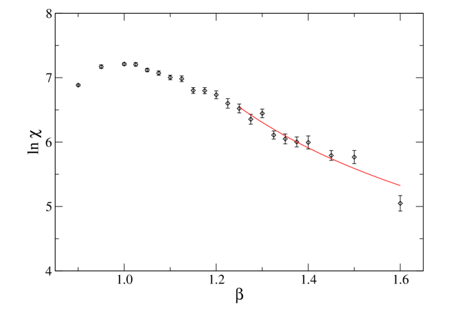
Figure 6: Thermal scaling of the polarisability of the random graph $F$ model for graphs with $N_{2}=30\,000$ sites. The curve shows a fit of the function (15) to the data, where $\beta_{c}=\ln 2$ and $\rho=1/2$ have been kept fixed.

The requirements of a proper thermal scaling analysis of the polarisability resulting from these observations are almost impossible to fulfil: one has to keep enough distance from the critical point for the linear extent of the graph to be large compared to the correlation length of the matter part to keep finite-size effects under control and, on the other hand, one should not proceed too deep into the ordered phase such as not to leave the thermal scaling region in the vicinity of the critical point. Thus, one would have to go to huge graph sizes to get rid of these constraints to a practically acceptable extent. Nevertheless, we attempt a thermal scaling analysis of the polarisability from simulations of graphs of size $N_{2}=30\,000$ with inverse temperatures ranging from $\beta=0.9$ up to $\beta=1.6$ taking about $800\,000$ measurements at each $\beta$. From the square-lattice results one expects the scaling form [weigel:05a, ],

$$\ln\chi(\beta)\sim A_{\chi}+B_{\chi}(\beta-\beta_{c})^{-\rho},$$ (15)

which should hold for $\beta\rightarrow\beta_{c}^{+}$ as $N_{2}\rightarrow\infty$ and where logarithmic corrections have already been omitted. We find it impossible to reliably fit all four of the parameters involved in Eq. (15) to the available data. Varying the starting values we find a multitude of local minima of the $\chi^{2}$ distribution, such that virtually any result can be “found” for $\beta_{c}$ and $\rho$ in this way. Fixing one or the other of the two parameters at the expected values $\beta_{c}=\ln 2$ or $\rho=1/2$, the fits become more stable. The dependency on the range of included values of $\beta$ is found to be rather small and for $\beta\geq 1.25$ we arrive at the fit parameters $A_{\chi}=-101(4662)$, $B_{\chi}=106(4662)$, $\rho=0.02(103)$, and $Q=0.03$, for $\beta_{c}$ fixed at $\ln 2$ or at the parameters $A_{\chi}=-86(1083)$, $B_{\chi}=324(5744)$, $\beta_{c}=-11(147)$, and $Q=0.04$, with $\rho$ fixed at $1/2$. Obviously both fits are not very useful, such that we are finally forced to fix both parameters, $\beta_{c}$ and $\rho$, at their expected values to find $A_{\chi}=0.91(41)$, $B_{\chi}=4.20(33)$, and $Q=0.03$. This fit is shown in Fig. 6 together with the simulation data. Thus, the best we can conclude about the thermal scaling behaviour of the polarisability is that there is no obvious contradiction with the expectations concerning the parameters $\beta_{c}$ and $\rho$. However, in view of the fact that already for the regular lattice model thermal scaling fits were not at all easily possible [weigel:05a, ], this finding is probably not too astonishing.

4 Geometrical properties

The annealed nature of disorder applied to the vertex model via its placement onto dynamical $\phi^{4}$ random graphs induces a back-reaction of the matter variables onto the underlying geometry and thus a possible change in the (local and global) geometrical properties of the graphs. Since the general mechanism of matter back-reaction onto the graphs is the tendency to minimise interfaces between pure-phase regions of the matter variables, a strong coupling between matter and graph variables is generically only expected if the combined system of spin model and underlying geometry is critical. Thus, the universal graph properties such as the graph-related critical exponents should remain at the values of pure Euclidean quantum gravity, unless the coupled matter system has a divergent correlation length [ambjorn:93b, ]. As indicators for changes of the geometry of the coupled system, we consider the co-ordination number distribution as a typical local property, as well as the string susceptibility exponent and the Hausdorff dimension as global geometrical features.

4.1 The co-ordination number distribution

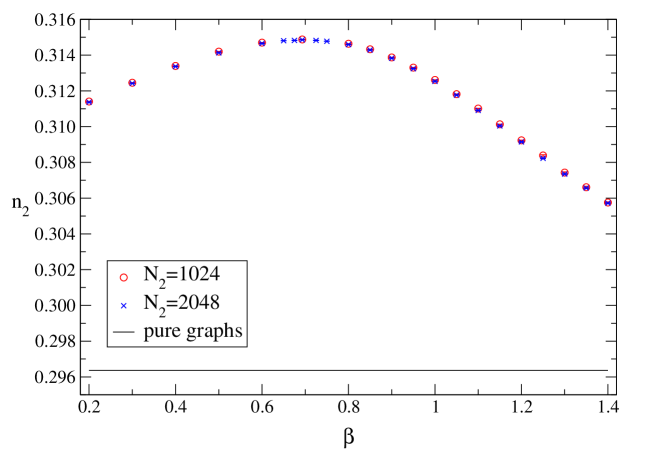
Figure 7: Fraction $n_{2}$ of faces of length two of planar $\phi^{4}$ “regular” random graphs with a coupled $F$ model as a function of the inverse temperature $\beta$. The drawn error bars are mostly covered by the size of the symbols. The solid line shows the value of $n_{2}$ for the case of pure $\phi^{4}$ random graphs of $N_{2}=2048$ sites.

The distribution of co-ordination numbers of the quadrangulations, which has been extensively considered for the case of pure $\phi^{4}$ graphs [doktor, ], could be possibly altered by the back-reaction of a coupled matter model. In particular, for the case of the vertex model considered here, the ice rule forbids certain link-flip update moves and thus changes the distribution $P_{N_{2}}(q)$ of co-ordination numbers. The vertex configurations forbidden by the ice rule effectively carry infinite energy, such that they stay excluded even in the infinite-temperature limit $\beta\rightarrow 0$. Thus, in contrast to, e.g., an Ising model a full decoupling of graph and matter variables for high temperatures does not occur here due to the entropic instead of energetic nature of the matter-graph back reaction.

From our numerical simulations we find that on the scale of the whole distribution $P_{N_{2}}(q)$ no changes as a function of the inverse simulation temperature $\beta$ can be distinguished and the distribution looks identical to that of pure planar $\phi^{4}$ graphs [doktor, ]. However, $P_{N_{2}}(q)$ can be determined to high precision, and concentrating on a single point of the distribution, e.g., $q=2$, a clear variation with the inverse temperature $\beta$ can be resolved, cf. Fig. 7. Also, in terms of the quoted statistical errors, which are of the order of $10^{-5}$ for the measurements of $n_{2}\equiv P_{N_{2}}(2)$, the pure graph result of $n_{2}=0.296\,365(32)$ for $N_{2}=2048$ [doktor, ] is very far away from the whole of the shown variation of the $F$ model case. We find a peak of $n_{2}$ around $\beta\approx 0.7$ with only rather small variations with the size of the considered graph. A similar peak of the fraction $P_{N_{2}}(3)$ of three-faces for different spin models coupled to dynamical triangulations has been observed before, see Ref. [baillie, ].

Since a pronounced back-reaction of the matter variables onto the underlying graphs is only expected at criticality, we interpret the location of the observed peak of $n_{2}(\beta)$ as a pseudo-critical point $\beta_{n_{2}}$ which should scale to the asymptotic critical coupling $\beta_{c}=\ln 2$. As for the thermal scaling analysis of Sec. 3.2, the precise location of the maxima can be determined from the simulation data via reweighting. This has been done for the data from simulations of graphs of sizes between $N_{2}=256$ and $N_{2}=4096$ sites with time series of lengths between $8\times 10^{5}$ and $4\times 10^{6}$ measurements. We find only very small changes of this peak position on variation of the size of the graphs, such that within the present statistical errors $\beta_{n_{2}}$ can be considered constant. Thus, we do not perform a finite-size scaling fit to the data of the peak locations, but instead quote the result from the largest considered lattice as an estimate for the asymptotic critical coupling, namely

$$\beta_{n_{2}}=0.6894(54),$$ (16)

resulting from the simulations for $N_{2}=4096$. This is in nice agreement with the expected value of $\beta_{c}=\ln 2\approx 0.693$ and almost two orders of magnitude more precise than the results found above from the scaling of the polarisability peak locations.

4.2 The string susceptibility exponent

In the grand-canonical ensemble of the dynamical polygonifications model the string susceptibility exponent $\gamma_{s}$ governs the leading singularity of the partition function for spherical graphs via $Z(\mu)\sim(\mu-\mu_{0})^{2-\gamma_{s}}$ [ambjorn:book, ], where $\mu$ denotes the chemical potential accounting for the cost of the insertion of a new vertex. Thus, a direct measurement of $\gamma_{s}$ requires computationally demanding simulations with a varying number of polygons or graph vertices. Additionally, since a shift of $\gamma_{s}$ due to the presence of some matter variables can only be expected at criticality, a numerical setup for the detection of such a change needs to tune two coupling constants, namely $\mu$ and $\beta$, to criticality. Due to the combination of these two problems a reliable estimation of $\gamma_{s}$ from grand-canonical Monte Carlo simulations has proved difficult, see e.g. Ref. [ambjorn:86, ].

It could be shown, however, that the string susceptibility exponent is related to the “baby-universe” structure of the dynamical polygonifications [jain:92a, ]. This observation can be turned into a method for the determination of $\gamma_{s}$ from simulations at a fixed number of polygons or graph vertices (canonical ensemble) [ambjorn:93b, ]. The basic building blocks of this “‘baby-universe” structure are taken as so-called “minimal-neck baby universes” (minBUs), which we define as subgraphs which typically contain a “macroscopic” number of vertices, but are connected to the main graph body by only four links for the case of dynamical quadrangulations. A simple decomposition argument of the graphs into “baby universes” yields the following scaling relation for the distribution $\langle n_{N_{2}}(B)\rangle$ of volumes $B$ contained in minBUs of the ensemble of pure graphs of size $N_{2}$ [ambjorn:93b, ],

$$\langle n_{N_{2}}(B)\rangle\sim N_{2}^{2-\gamma_{s}}[B(N_{2}-B)]^{\gamma_{s}-2},$$ (17)

where $B\gg 1$ and $N_{2}-B\gg 1$ is assumed. Also, it can be shown that the same relation should hold for the case of $C<1$ conformal matter coupled to the polygonifications or dual graphs with $\gamma_{s}$ then denoting the corresponding dressed string susceptibility exponent [jain:92a, ]. For the limiting case $C=1$, on the other hand, it is argued in Ref. [jain:92a, ] that the distribution of minBUs should acquire logarithmic corrections and look like,

$$\langle n_{N_{2}}(B)\rangle\sim N_{2}^{2-\gamma_{s}}[B(N_{2}-B)]^{\gamma_{s}-2}[\ln B\,\ln(N_{2}-B)]^{\kappa},$$ (18)

with $\kappa=-2$. An estimate $\bar{n}_{N_{2}(B)}$ for the volume distribution of minBUs can be easily found numerically from a decomposition of the graphs into “baby universes”. When the minBU surgery algorithm (cf. Refs. [prep, , doktor, ]) is applied, such an estimate can even be produced as a simple by-product of the updating scheme. Then, an estimate for $\gamma_{s}$ can be found from a fit of the conjectured functional form (17) or (18) to the estimated distribution $\bar{n}_{N_{2}(B)}$ [ambjorn:93b, ]. In order to honour the constraints $B\gg 1$ and $N_{2}-B\gg 1$ of Eqs. (17) and (18) one has to introduce cut-offs $B_{\mathrm{min}}$ and $B_{\mathrm{max}}$, such that only data with $B_{\mathrm{min}}\leq B\leq B_{\mathrm{max}}$ are included in the fit. Here, the choice of the lower cut-off $B_{\mathrm{min}}$ is found to be much more important for the outcome of the fit than the choice of $B_{\mathrm{max}}$. We use the following recipe for the determination of the cut-offs: as a rule of thumb, we choose $B_{\mathrm{max}}=N_{2}/8$, which has turned out to be a good initial guess for most situations. With $B_{\mathrm{max}}$ fixed, the lower cut-off $B_{\mathrm{min}}$ is steadily increased from $B_{\mathrm{min}}\approx 0$, monitoring the effect of those increases on the resulting fit parameters, especially the estimated string susceptibility exponent $\gamma_{s}$. Finally, with the resulting value of $B_{\mathrm{min}}$ fixed, a second adaption of $B_{\mathrm{max}}$ is attempted, usually changing $B_{\mathrm{max}}$ by factors of two or one half. Additionally, the quality-of-fit parameter $Q$ is utilised as an indicator of whether neglected corrections to scaling are important for the considered window of minBU volumes $B$. As far as corrections to the leading scaling behaviour are concerned, it is speculated in Ref. [ambjorn:93b, ] that a good effective description of the leading correction term results from the substitution $B^{\gamma_{s}-2}\rightarrow B^{\gamma_{s}-2}[1+D_{\gamma_{s}}/B]$. Hence, the actual fits were performed to the functional form

$$\ln\bar{n}_{N_{2}}(B)=A_{\gamma_{s}}+(\gamma_{s}-2)\ln\left[B(N_{2}-B)\right]+\frac{D_{\gamma_{s}}}{B},$$ (19)

for $C<1$, resp. to the form

$$\ln\bar{n}_{N_{2}}(B)=A_{\gamma_{s}}+(\gamma_{s}-2)\ln[B(N_{2}-B)]+\kappa\ln[\ln B\ln(N_{2}-B)]+\frac{D_{\gamma_{s}}}{B},$$ (20)

for the limiting case of $C=1$. Here, the dependency on the total volume $N_{2}$ has been condensed into the constant $A_{\gamma_{s}}$. Note that both of these fits are linear and the number of data points is of the order of $10^{3}$ for the lattice sizes we have considered, such that a fit with four independent parameters is not unrealistic. In Eq. (20) we keep $\kappa$ as a free parameter since the value $\kappa=-2$ is only a conjecture and, additionally, further corrections to scaling can be covered in an effective way by letting $\kappa$ vary.

4.2.1 Results for pure $\phi^{4}$ graphs

Matrix model calculations for pure, planar dynamical triangulations yield the exact result $\gamma_{s}=-1/2$, cf. Ref. [ambjorn:book, ]. As a gauge for the method and as a check for the expected universality of $\gamma_{s}$ with respect to the change from triangulations to quadrangulations, we apply the described technique first to the case of pure $\phi^{4}$ random graphs. We adapt the lower and upper cut-offs $B_{\mathrm{min}}$ and $B_{\mathrm{max}}$ iteratively as described above, taking into account that the usual error estimates of least-squares fits of (19) to the data could be misleading due to the apparent correlations of the points of $\bar{n}_{N_{2}}(B)$ for different sizes $B$ of the minBUs, which generically lead to an underestimation of variances. We refrain from an additional extrapolation of the resulting estimates of $\gamma_{s}$ towards $B_{\mathrm{min}}\rightarrow\infty$ suggested by the authors of Ref. [ambjorn:93b, ] since we do not see a proper justification for a specific extrapolation ansatz and in general find extrapolations of noisy (and here also strongly correlated) data questionable.

Table 4: Parameters of fits of (19) to the simulation data for the distribution $\bar{n}_{N_{2}}(B)$ of minBUs for pure $\phi^{4}$ random graphs. The small values of the quality-of-fit parameter $Q$ for the two largest graph sizes are a side effect of the cross-correlations in $\bar{n}_{N_{2}}(B)$.

$N_{2}$	$B_{\mathrm{min}}$	$B_{\mathrm{max}}$	$A_{\gamma_{s}}$		$\gamma_{s}$		$D_{\gamma_{s}}$		$Q$
1024	60	128	18.	36(49)	$-0$.	474(40)	$-2$.	9(30)	0.79
2048	70	256	20.	34(14)	$-0$.	495(10)	$-3$.	8(12)	0.56
4096	70	512	22.	030(90)	$-0$.	4915(63)	$-3$.	78(74)	0.05
8192	100	1024	23.	853(72)	$-0$.	4977(47)	$-4$.	80(87)	0.04

Statistically reliable error estimates for $\gamma_{s}$ are found by jackknifing over the whole fitting procedure: first the upper and lower cut-offs in $B$ are determined as described using the full estimate $\bar{n}_{N_{2}}(B)$. Then, of the order of ten jackknife blocks are built from the time series the estimate $\bar{n}_{N_{2}}(B)$ is based on and fits with the same constant cut-offs are performed for each block to yield jackknife-block estimates of $\gamma_{s}$ and the other fit parameters. Table 4 summarises the final results for pure $\phi^{4}$ graphs of sizes $N_{2}=1024$ up to $N_{2}=8192$, taking about $10^{9}\times N_{2}$ minBUs into account for each graph size. Obviously, finite-size effects are relatively weak here, and we quote as final result the value for $N_{2}=8192$, $\gamma_{s}=-0.4977(47)$, which is perfectly compatible with $\gamma_{s}=-1/2$.

4.2.2 Results for the $F$ model case

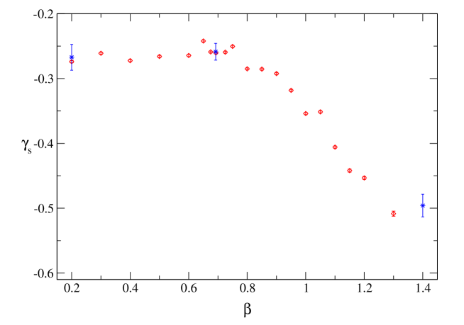
Figure 8: Estimates of the string susceptibility exponent $\gamma_{s}$ from fits of (19) to the measured distribution of minBUs for graphs of size $N_{2}=2048$ coupled to the $F$ model. The displayed error bars do not represent the full statistical error. The true amount of statistical fluctuations is indicated by the three data points with larger error bars at couplings $\beta=0.2$, $\beta=\ln 2$, and $\beta=1.4$, where the errors have been evaluated by a full jackknife analysis. Note that the displayed exponent estimates in the high-temperature phase are effective exponents since there are large finite-size corrections (see text).

For the case of the $F$ model coupled to the $\phi^{4}$ graphs, we expect a variation of the string susceptibility exponent $\gamma_{s}$ with the inverse temperature $\beta$ of the $F$ model. Since the whole high-temperature phase is critical with central charge $C=1$, in the thermodynamic limit $\gamma_{s}$ should vanish for all $\beta\leq\beta_{c}=\ln 2$, whereas in the non-critical ordered phase the exponent should stick to the pure quantum gravity value of $\gamma_{s}=-1/2$. To get an overview of the temperature dependence of $\gamma_{s}$ we measured the distribution $\bar{n}_{N_{2}}(B)$ of minBUs over an inverse temperature range of $0.2\leq\beta\leq 1.4$ for graphs of size $N_{2}=2048$ and performed fits of the functional form (19) to the data to extract $\gamma_{s}$ [thus first neglecting the possibility of additional logarithmic corrections indicated in Eq. (20)]. The resulting estimates for $\gamma_{s}$ presented in Fig. 8 show a plateau value of $\gamma_{s}\approx-0.25$ within the critical phase $\beta\leq\ln 2$ and a slow drop down to $\gamma_{s}\approx-0.5$ at $\beta=1.4$ in the low-temperature phase. Note that the error bars displayed in Fig. 8 are those resulting from the fit procedure itself and are thus not representing the full statistical variation due to the above mentioned cross-correlations between the values of $\bar{n}_{N_{2}}(B)$. For comparison the correct error bars as obtained from a more elaborate jackknife analysis are shown for three selected $\beta$-values, which are discussed in more detail below. As will be shown there, the fact that $\gamma_{s}$ is found to be still considerably smaller than zero in the high-temperature phase is due to a finite-size effect. We do not employ the corrected fit (20) at this point, which is found to be unstable for the small graph size considered here.

More precise estimates for $\gamma_{s}$ are found from a FSS study of three series of simulations, one at the critical point $\beta_{c}=\ln 2$, one in the critical high-temperature phase at $\beta=0.2$ and one deep in the ordered phase at $\beta=1.4$. For the latter case, the exponential slowing down of the combined link-flip and surgery dynamics of the graphs reported in Refs. [prep, , doktor, ] limited the maximum accessible graph size to $N_{2}=16\,384$, while for the simulations at the critical point and in the high-temperature phase graphs with up to $N_{2}=65\,536$ sites were considered. At $\beta=1.4$, this maximal size is anyway sufficient since we find no finite-size drift in the estimate for $\gamma_{s}$ with increasing graph sizes, all results being compatible with the conjectured value of $\gamma_{s}=-1/2$. Thus, as our final estimate for $\beta=1.4$ we report the value found for $N_{2}=16\,384$, $\gamma_{s}=-0.478(17)$. For the quoted statistical error estimates the jackknifing procedure described above for pure dynamical $\phi^{4}$ graphs was used, thus taking full account of the present fluctuations.

At the critical point $\beta_{c}=\ln 2$ fits of the form (19) without logarithmic corrections show considerable finite-size effects, with $\gamma_{s}$ slowly increasing with the graph size. For the largest graph size considered, $N_{2}=65\,536$, the thus found estimate $\gamma_{s}=-0.2075(17)$ is still far away from the expected result $\gamma_{s}=0$. Taking the logarithmic corrections into account, however, these results can be considerably improved, with the numerical estimates for $\gamma_{s}$ now being fully consistent with the theoretical prediction. The parameters of fits of the corresponding functional form (20) are collected in Table 5. Including this correction, no further finite-size dependence of the estimate $\gamma_{s}$ is visible. The occurring values for the “correction exponent” $\kappa$ are not too far away from and indeed statistically compatible with the conjectured value of $\kappa=-2$. Since for the case of $N_{2}=65\,536$ only a much shorter time series than for the smaller graph sizes was recorded, we present as our final estimate of the critical value of $\gamma_{s}$ the result at $N_{2}=32\,768$, $\gamma_{s}=0.013(70)$.

Table 5: Parameters of fits of the form (20) to the distribution $\bar{n}_{N_{2}}(B)$ of minBUs for $\phi^{4}$ random graphs coupled to the $F$ model at $\beta=\beta_{c}=\ln 2$.

$N_{2}$	$B_{\mathrm{min}}$	$B_{\mathrm{max}}$	$A_{\gamma_{s}}$		$\gamma_{s}$		$\kappa$		$D_{\gamma_{s}}$
16 384	100	2048	25.	7(15)	$0$.	05(13)	$-1$.	97(89)	$-10$.	9(69)
32 768	110	4096	27.	08(93)	$0$.	013(70)	$-1$.	80(50)	$-12$.	6(47)
65 536	120	4096	27.	5(14)	$-0$.	05(12)	$-1$.	27(82)	$-6$.	9(71)

Finally, in the high-temperature phase at $\beta=0.2$ the simulation results behave very similar to the critical point case. When applying fits of the form (19) without logarithmic corrections, considerable finite-size effects are found, and the approach of the resulting exponent estimates $\gamma_{s}$ to the expected value of $\gamma_{s}=0$ is very slow. On the other hand, the estimates resulting from fits of the form (20) to the data are compatible with $\gamma_{s}=0$ for the larger of the considered graph sizes. For $N_{2}=32\,768$ we find $\gamma_{s}=-0.041(73)$, $\kappa=-1.38(47)$, $Q=0.05$ with cut-offs $B_{\mathrm{min}}=100$ and $B_{\mathrm{max}}=2048$. To complete the picture, it should be mentioned that the functional form (20) does not fit the data in the low-temperature phase at $\beta=1.4$ well and does not give estimates of $\gamma_{s}$ compatible with $\gamma_{s}=0$, in agreement with theoretical expectations.

4.3 The Hausdorff dimension

The internal Hausdorff dimension $d_{h}$ of the dynamical polygonifications is one of its most striking features. Apart from the physical implications, its large value causes a quite inconvenient obstacle for the numerical analysis of the model, namely the comparable smallness of the effective linear extent of the graphs at a given total volume $N_{2}$ as compared to flat lattices. As matter variables are coupled to the dynamical graphs, the strong coupling between graph and matter variables at criticality could lead to a change of the fractal dimension of the lattices. In a phenomenological scaling picture, such a strong coupling of matter and geometry should set in as soon as the correlation length of the matter system becomes comparable to the intrinsic length scale of the graphs or polygonifications. For conformal minimal matter, there has been quite some debate about how $d_{h}$ should depend on the central charge $C$ of the coupled matter system, see, e.g., Refs. [catterall:95a, , ambjorn:95d, , ambjorn:95e, , ambjorn:97b, , ambjorn:98b, , ambjorn:98d, ]. For $C=0$ the result $d_{h}=4$ is exact [kawai, ]. Furthermore, the branched polymer model [ambjorn:86, ], describing the $C\rightarrow\infty$ limit [david:97a, ], yields $d_{h}=2$ (see, e.g., Ref. [jurkiewicz:97a, ]). For the intermediate region $0\leq C\leq 1$ two differing conjectures have been made for $d_{h}$, namely [watabiki:93a, ]

$$d_{h}=2\frac{\sqrt{25-C}+\sqrt{49-C}}{\sqrt{25-C}+\sqrt{1-C}}\;\stackrel{{\scriptstyle C\rightarrow 1}}{{\longrightarrow}}\;2(1+\sqrt{2})\approx 4.83,$$ (21)

and [ishibashi:94a, ]

$$d_{h}=\frac{24}{\sqrt{1-C}(\sqrt{1-C}+\sqrt{25-C})}\;\stackrel{{\scriptstyle C\rightarrow 1}}{{\longrightarrow}}\;\infty.$$ (22)

All numerical investigations up to now, on the other hand, are consistent with a constant $d_{h}=4$ for $0\leq C\leq 1$ [ambjorn:95d, , ambjorn:95e, , ambjorn:97a, , ambjorn:98d, ]. Naturally, the limiting case $C=1$ considered here is of special interest for the investigation of the transition to the branched polymer regime $C\gg 1$. Numerically, it has proved exceptionally difficult to extract the Hausdorff dimensions from the statistics of the practically accessible graph sizes [billoire:86a, , agishtein:91b, , ambjorn:95e, ]. Only more recently, the development and application of suitable FSS techniques allowed for a more successful and precise determination of $d_{h}$ [catterall:95a, , ambjorn:97b, , ambjorn:98d, ].

4.3.1 Scaling and the two-point function

The fractal structure of the polygonifications is encoded in their geometrical two-point function. Here, different definitions are possible. While in Eq. (9) a definition in terms of the vertices of the graphs has been used, here, instead, the number of vertices of the quadrangulation is counted. Thus, we define the geometrical two-point function $G_{11}^{N_{2}}(r)$ as the average number of vertices of the polygonifications at a distance $r$ from a marked vertex, where “distance” denotes the unique minimal number of links one has to traverse to connect both vertices. Since the intrinsic length of the model scales as $N_{2}^{1/d_{h}}$ by definition of the internal Hausdorff dimension $d_{h}$, from the usual FSS arguments one can make the following scaling ansatz (see, e.g., Ref. [catterall:95a, ]),

$$G_{11}^{N_{2}}(r)\sim N_{2}^{\alpha}\,F(r/N_{2}^{1/d_{h}}),$$ (23)

i.e., $G_{11}^{N_{2}}(r)$ is a generalised homogeneous function and one can define a scaling function $F(x)$ of the single scaling variable $x=r/N_{2}^{1/d_{h}}$ and a critical exponent $\alpha$. Due to the obvious constraint $N_{2}=\sum_{r}G_{11}^{N_{2}}(r)$, the exponent $\alpha$ is not independent, but given by $\alpha=1-1/d_{h}$. It turns out that for practical purposes the scaling variable has to be shifted to yield reliable results, see, e.g., Refs. [ambjorn:97b, , ambjorn:98b, , ambjorn:99a, ]. The necessity of such a shift can be most easily seen by a phenomenological scaling discussion of the mean extent defined by

$$\langle r\rangle_{N_{2}}=\frac{1}{N_{2}}\sum_{r}r\,G_{11}^{N_{2}}(r)\sim F_{0}N_{2}^{1/d_{h}},$$ (24)

with $F_{0}=\sum_{r}F(r)$. On general grounds, one expects the presence of analytical scaling corrections,

$$\frac{\langle r\rangle_{N_{2}}}{N_{2}^{1/d_{h}}}\sim F_{0}-\frac{a}{N_{2}^{1/d_{h}}}-\frac{b}{N_{2}^{2/d_{h}}}+\cdots.$$ (25)

Combining the terms proportional to $1/N_{2}^{1/d_{h}}$ on both sides, the mean extent is found to be $\langle r+a\rangle_{N_{2}}\sim F_{0}N_{2}^{1/d_{h}}+O(N_{2}^{-1/d_{h}})$. Thus, to incorporate first-order corrections to scaling, the ansatz (23) is replaced by

$$G_{11}^{N_{2}}(r)\sim N_{2}^{\alpha}\,F[(r+a)/N_{2}^{1/d_{h}}],$$ (26)

i.e., the scaling variable is now defined to be $x=(r+a)/N_{2}^{1/d_{h}}$.

4.3.2 Scaling of the maxima

The two-point function $G_{11}^{N_{2}}(r)$ exhibits a peak at intermediate distances and declines exponentially as $r\rightarrow\infty$, cf. Fig. 10 below. From the scaling ansatz (26) one infers the following leading scaling behaviour of the position and height of the maxima,

$$\begin{array}[]{rcl}r_{\mathrm{max}}+a&=&A_{r}N_{2}^{1/d_{h}},\\ G_{11}^{N_{2}}(r_{\mathrm{max}})&=&A_{n}N_{2}^{1-1/d_{h}}+B_{n}.\end{array}$$ (27)

Since the location and height of these maxima can be determined numerically from simulation data, these relations can be used to estimate the intrinsic Hausdorff dimension $d_{h}$. A technical difficulty is given by the fact that $r$ can only take on integer values for the discrete graphs considered. This problem is circumvented by a smoothing out of the vicinity of the maximum by a fit of a low-order polynomial to $G_{11}^{N_{2}}(r)$ around its maximum. For practical purposes, we find a fourth-order polynomial sufficient for this fit. Reliable error estimates are found by jackknifing over this whole fitting procedure, where the individual statistical errors of the data points included in the fits are taken to be equal. Thus, one arrives at estimates for the peak locations $r_{\mathrm{max}}$ and heights $G_{11}^{N_{2}}(r_{\mathrm{max}})$ as a function of the graph size $N_{2}$, to which then the functional forms of Eq. (27) are fitted. The effect of neglected FSS corrections is accounted for by successively dropping data points from the small-$N_{2}$ side. For simulations of pure $\phi^{4}$ random graphs, in this way we find the value of $d_{h}$ to steadily increase on omitting more and more points. For the range $N_{2}=4096$ up to $N_{2}=32\,768$ we thus arrive at the estimates $d_{h}=3.803(28)$, $Q=0.22$ from the scaling of the peak locations and $d_{h}=3.814(63)$, $Q=0.44$ from the peak heights. Both estimates are still noticeably away from the asymptotic values $d_{h}=4$, owing to the neglect of higher-order correction terms [catterall:95a, ]. We note that introducing the shift parameter $a$ already largely improved the estimates, since fixing $a=0$ we arrive at $d_{h}=3.4313(20)$ from the peak locations. Further improvement is gained from the inclusion of the next-order correction term for the scaling of the peak locations,

$$r_{\mathrm{max}}+a=A_{r}N_{2}^{1/d_{h}}+B_{r}N_{2}^{-1/d_{h}},$$ (28)

which yields an estimate of $d_{h}=3.964(42)$, $Q=0.24$ for the range $N_{2}=512,\ldots,32\,768$, in perfect agreement with $d_{h}=4$.

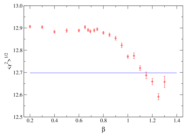
Figure 9: Root mean square extent $\langle r^{2}\rangle^{1/2}$ of regular $\phi^{4}$ random graphs with $N_{2}=2048$ sites coupled to the $F$ model. The horizontal line indicates the root mean square extent of pure $\phi^{4}$ random graphs of the same size.

For random $\phi^{4}$ graphs coupled to the $F$ model, we find a small dependence of the root mean square extent on the inverse temperature $\beta$ of the coupled $F$ model and also a slight shift of $\langle r^{2}\rangle^{1/2}$ as compared to the case of pure $\phi^{4}$ random graphs, cf. Fig. 9. Thus, one might expect the Hausdorff dimension $d_{h}$ to be temperature dependent, too. We performed simulations for three inverse temperatures, namely $\beta=0.2$, $\beta=\ln 2$ and $\beta=1.4$, covering the cases of interest. The results for $d_{h}$ from fits of the functional form (27) to the data are found to steadily increase on omitting more and more points from the small-$N_{2}$ side. In agreement with the case of pure $\phi^{4}$ graphs, the final estimates for $d_{h}$ are found to be significantly smaller than $d_{h}=4$ for all three inverse temperatures due to the presence of higher-order corrections to scaling. For the peak heights, this analysis yields the estimates $d_{h}=3.446(68)$ for $\beta=0.2$, $d_{h}=3.426(92)$ for $\beta=\ln 2$ and $d_{h}=3.94(23)$ for $\beta=1.4$, where the rather different result for $\beta=1.4$ again indicates the presence of competing local minima in the $\chi^{2}$ distribution. The found higher-order scaling corrections are resolved by using the fit ansatz (28) for the peak locations. Here, we do not find a significant sensitivity of the parameter estimates on the cut-off $N_{2,\mathrm{min}}$ and for all three inverse temperatures the resulting values for $d_{h}$ are in agreement with the pure gravity value $d_{h}=4$, cf. the fit data collected in Table 6.

Table 6: Parameters of fits of the form (28) to the peak locations of the two-point functions of the random graph $F$ model. The maximum graph size was $N_{2}=65\,536$ for $\beta=0.2$ and $\beta=\ln 2$ and $N_{2}=32\,768$ for $\beta=1.4$.

$\beta$	$N_{2,\mathrm{min}}$	$A_{r}$		$B_{r}$		$a$		$d_{h}$		$Q$
0.2	2048	2.	34(43)	9.	2(39)	5.	5(21)	4.	13(20)	0.	86
$\ln 2$	2048	1.	96(39)	5.	6(43)	3.	7(20)	3.	93(21)	0.	11
1.4	1024	2.	18(49)	6.	0(37)	4.	4(22)	4.	07(26)	0.	44

4.3.3 Scaling of the mean extent

As an alternative to the scaling of the maxima of the two-point function, one can also consider the behaviour of mean properties of the distribution $G_{11}^{N_{2}}(r)$, especially the scaling of the mean extent (24). Taking the next sub-leading analytic correction term into account, we make the scaling ansatz

$$\langle r+a\rangle_{N_{2}}=A_{\langle r\rangle}N_{2}^{1/d_{h}}+B_{\langle r\rangle}N_{2}^{-1/d_{h}}.$$ (29)

We again consider the case of pure $\phi^{4}$ graphs first. When fixing $B_{\langle r\rangle}=0$ and adapting the lower cut-off $N_{2,\mathrm{min}}$, the resulting values of $d_{h}$ are significantly too small in terms of the statistical errors with an obvious tendency to increase as more and more of the points from the small-$N_{2}$ side are omitted. On the other hand, including the correction term of Eq. (29) largely reduces the dependency on the cut-off $N_{2,\mathrm{min}}$. For $N_{2,\mathrm{min}}=256$ we find $d_{h}=3.90(15)$, $Q=0.01$, in nice agreement with $d_{h}=4$. Here, the fits become very unstable as less points are included; this explains the use of the cut-off $N_{2,\mathrm{min}}=256$, although the quality-of-fit is rather poor.

The authors of Ref. [ambjorn:97b, ] have proposed a different and less conventional method to extract $a$ and $d_{h}$ from data of the mean extent, which they claim to be especially well suited for obtaining high-precision results. They consider the combination $R_{a,N_{2}}(d_{h})\equiv\langle r+a\rangle_{N_{2}}N_{2}^{-1/d_{h}}$, and evaluate it for a series of simulations for different graph sizes $N_{2}$. Then, for a given $a$ and for each pair $(N_{2}^{i},N_{2}^{j})$ they define $d_{h}^{ij}(a)$ such that $R_{a,N_{2}^{i}}(d_{h}^{ij})=R_{a,N_{2}^{j}}(d_{h}^{ij})$, i.e.,

$$d_{h}^{ij}(a)=\frac{\ln N_{2}^{i}-\ln N_{2}^{j}}{\ln(\langle r\rangle_{N_{2}^{i}}+a)-\ln(\langle r\rangle_{N_{2}^{j}}+a)}.$$ (30)

By a binning technique, an error estimate $\sigma(d_{h}^{ij})$ is evaluated and the estimates $d_{h}^{ij}(a)$ are averaged over all pairs $(N_{2}^{i},N_{2}^{j})$ of volumes, $\bar{d}_{h}(a)=\sum_{i<j}d_{h}^{ij}(a)/{\mathcal{N}}$, where ${\mathcal{N}}$ denotes the number of pairs $(N_{2}^{i},N_{2}^{j})$. Then, the optimal choice $a_{\mathrm{opt}}$ of the shift is found by minimising

$$\chi^{2}(a)=\sum_{i<j}\frac{[d_{h}^{ij}(a)-\bar{d}_{h}(a)]^{2}}{\sigma^{2}[d_{h}^{ij}(a)]},$$ (31)

being accompanied by an optimal estimate $\bar{d}_{h}(a_{\mathrm{opt}})$. The authors of Ref. [ambjorn:97b, ] suggest to estimate the statistical error of this final estimate by considering the variation of $(a,\bar{d}_{h})$ in an interval of $a$ around $a_{\mathrm{opt}}$ defined by $\chi^{2}(a)<\min[1,2\chi^{2}(a_{\mathrm{opt}})]$. We implemented this procedure to compare with the results of the fits to Eq. (29) with $B_{\langle r\rangle}=0$ for the case of pure $\phi^{4}$ graphs. We find the ad hoc assumption for the estimation of the errors of $(a,\bar{d}_{h})$ not adequate. Instead, we apply a second-order jackknifing technique (cf. Ref. [doktor, ]) to be able to give error estimates for $d_{h}^{ij}(a)$ as well as the final estimate $(a,\bar{d}_{h})$ which are found to be largely differing from those resulting from the rule $\chi^{2}(a)<\min[1,2\chi^{2}(a_{\mathrm{opt}})]$, ranging from four times smaller to ten times larger error estimates. The estimates of $d_{h}$ itself are found to be indeed slightly increased as compared to the fit method (which yielded estimates clearly smaller than $d_{h}=4$). This, however, can be traced back to the fact that the individual estimates $d_{h}^{ij}(a)$ all receive the same weight in the average $\bar{d}_{h}(a)$ above, irrespective of their precision, giving an extra weight to the results for larger graphs, which cannot be justified on statistical grounds. If, instead, we use a variance-weighted average

$$\bar{d}_{h}(a)=\frac{\sum_{i<j}d_{h}^{ij}(a)/\sigma^{2}[d_{h}^{ij}(a)]}{\sum_{i<j}1/\sigma^{2}[d_{h}^{ij}(a)]},$$ (32)

the resulting estimates for $d_{h}$ and $a$ are statistically equivalent to those found from the fits to (29). For a cut-off $N_{2,\mathrm{min}}=2048$, for instance, we find $\bar{d}_{h}=3.97(12)$ compared to $d_{h}=3.99(12)$ from a simple fit of the form (29) with $B_{\langle r\rangle}=0$. Thus, we do not find any special benefits of this computationally rather demanding method as compared to a plain fit to (29) with $B_{\langle r\rangle}=0$ and hence do not present further detailed results for this method.

For the case of the $F$ model coupled to the $\phi^{4}$ random graphs we proceeded as before, again using simulation data for $\beta=0.2$, $\beta=\ln 2$ and $\beta=1.4$. The results from fits of the mean extent $\langle r\rangle_{N_{2}}$ to the form (29) with $B_{\langle r\rangle}=0$ show very much the same behaviour as the results from the scaling of the maxima of the two-point function, with estimates of $d_{h}$ clearly below $d_{h}=4$ and slowly increasing as more and more points from the small-$N_{2}$ side are omitted from the fits. The outcomes of the method of Ref. [ambjorn:97b, ] described above, with the average (32) and the $\chi^{2}(a)$ rule replaced by a jackknife error estimate, are again very close to the fit results. Including the correction term of (29), i.e., relaxing the constraint $B_{\langle r\rangle}=0$, on the other hand, yields estimates consistent with $d_{h}=4$ for $\beta=0.2$ and $\beta=1.4$, however with rather large statistical errors, cf. the parameters collected in Table 7. Note that, as mentioned before, the results for $\beta=1.4$ are in general less precise than those for the other two inverse temperatures, which is due to the exponential slowing down of the combined link-flip and surgery dynamics in the low-temperature phase, cf. Ref. [prep, ]. The fit for $\beta=\ln 2$ settles down at a completely different minimum of the $\chi^{2}$ distribution, yielding an almost unchanged $d_{h}$ compared to the outcome of the corresponding fit without correction term. This underlines the fact that the complexity of the chosen fit is at least at the verge of being too high for the available data. Nevertheless, combining the data for $d_{h}$ from the presented methods and including the comparison to the pure gravity case, we find no reason to assume that $d_{h}$ differs from $d_{h}=4$ for the case of the $F$ model coupled to $\phi^{4}$ random graphs. At any rate, the values $d_{h}\approx 4.83$ and $d_{h}=\infty$ resulting from the analytical conjectures Eqs. (21) and (22) for $C=1$, respectively, are clearly incompatible with the results found here.

Table 7: Parameters of fits of the form (29) including the correction term to the mean extent of dynamical $\phi^{4}$ graphs coupled to the $F$ model at different inverse temperatures $\beta$.

$\beta$	$N_{2,\mathrm{min}}$	$A_{\langle r\rangle}$		$B_{\langle r\rangle}$		$a$		$d_{h}$		$Q$
0.2	512	2.	58(48)	11.	4(33)	7.	0(22)	4.	08(21)	0.	10
$\ln 2$	512	1.	37(22)	0.	4(29)	1.	1(12)	3.	45(14)	0.	41
1.4	512	2.	6(10)	9.	1(58)	6.	2(42)	4.	15(47)	0.	29

Finally, we note that the parameters $a$ and $d_{h}$ determined from the fits discussed above lead to a nice scaling collapse of the two-point functions $G_{11}^{N_{2}}(r)$ when re-scaled according to the scaling ansatz of Eq. (26). Figure 10 shows this collapse of distributions for the case of $\beta=0.2$ and the choice of parameters found from a fit to the form (29) with $B_{\langle r\rangle}=0$, i.e., $d_{h}=3.57(12)$ and $a=1.60(74)$. The visible deviations around the peaks of the distributions indicate the presence of higher-order corrections not incorporated into the scaling ansatz (26).

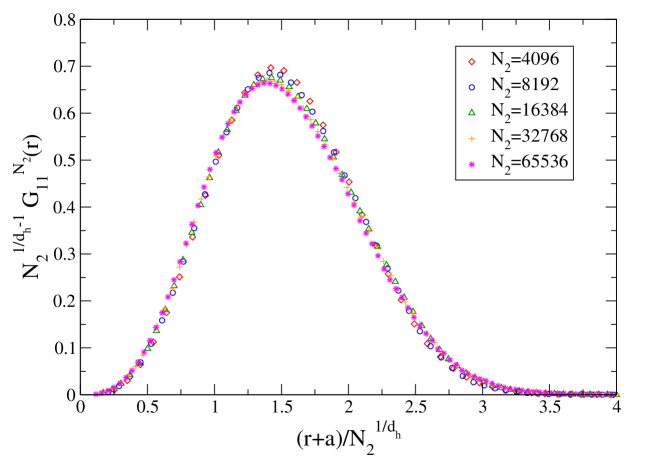
Figure 10: Scaling collapse of the two-point functions $G_{11}^{N_{2}}(r)$ of $\phi^{4}$ graphs coupled to the $F$ model at $\beta=0.2$, re-scaled according to Eq. (26) with $d_{h}=3.57$ and $a=1.60$.

5 Conclusions

The six-vertex $F$ model represents an example of the limiting case of a critical theory at the “barrier” of central charge $C=1$, where the Liouville approach to Euclidean quantum gravity in two dimensions breaks down [kpzddk, ] and the ensemble of planar random graphs coupled to such matter is at the verge of a presumable collapse towards a phase of minimally connected, tree-like surfaces termed “branched polymers” [david:97a, ]. At the same time, the family of ice-type vertex models of statistical mechanics includes as sub-classes a variety of well-known lattice spin models and combinatorial counting problems and hence the analysis of its coupling to two-dimensional Euclidean quantum gravity is that of a prototype model of statistical mechanics subject to annealed, correlated connectivity disorder from random graphs (see also Ref. [wj:04a, ]).

For studying the effect of a coupled six-vertex $F$ model, we generalised the well-established methods of simulating dynamical triangulations to the case of planar quadrangulations and the dual “fat” $\phi^{4}$ random graphs; the details of this simulational machinery will be presented in a forthcoming publication [prep, ]. We have analysed the critical and off-critical behaviour of this model using a series of extensive Monte Carlo simulations and subsequent finite-size and thermal scaling analyses. On the square lattice, this model undergoes an infinite-order phase transition of the Kosterlitz-Thouless type to an anti-ferroelectric phase of staggered order. Expecting similar ordering behaviour to occur for the model on a random quadrangulation, we generalised the corresponding staggered polarisation (the order parameter) to the random graph case by a duality transformation of the vertex model.

The scaling analysis of the simulation data is hampered by the presence of extraordinarily strong corrections, which can be traced back to the combined effect of the comparable smallness of the effective linear extents of the considered (two-dimensional) lattices due to their large fractal dimension close to four and the presence of logarithmic corrections generically expected for a $C=1$ critical point. Additionally, the form of the critical singularities for a Kosterlitz-Thouless phase transition severely limits the effectivity of the usual finite-size scaling techniques. General symmetry considerations imply that the $C=1$ critical point of the random-graph model should occur at the coupling $\beta_{c}=\ln 2$, which is quite remarkably identical to the critical coupling of the square-lattice model. Additionally, this is in agreement with a matrix model treatment of the system [zinn, , zinn-justin:03a, ]. Due to the aforementioned strength of scaling corrections, a precise determination of the critical coupling from the scaling of the polarisability alone is found to be hard. A comparison of the peak positions re-scaled according to the mean linear extents of the lattices between the random graph and square-lattice models [weigel:05a, ], however, shows that the finite-size scaling approaches of both models are indeed very similar, but with larger correction amplitudes for the random graph model. Subsequently, however, a precise and consistent estimate of the transition point could be extracted from the scaling of the co-ordination number distribution of the graphs. A cursory comparison of the scaling behaviour of the model for different ensembles regarding the inclusion of singular contributions in the graphs reveals that corrections to scaling increase as more and more singular contributions are included. This contrasts with the findings for pure gravity and Potts models coupled to the polygonifications model [ambjorn:95a, , doktor, ]. As far as the critical exponents related to the order parameter are concerned, a finite-size scaling analysis of the spontaneous polarisation and the polarisability at the asymptotic critical coupling yields critical exponents in good agreement with the predictions from the KPZ/DDK formula. An attempted thermal scaling analysis of the polarisability around its peak remains inconclusive due to the extraordinary magnitude of finite-size corrections. As a curiosity, we report the finding of a critical internal energy of the model, $U(\beta_{c})=1/3$, which is identical between the square-lattice and random graph cases.

Several aspects of the back-reaction of the matter variables onto the properties of the $\phi^{4}$ random graphs are analysed as a function of temperature. The distribution of co-ordination numbers of the quadrangulations can be determined very accurately. The fraction of quadrangulation sites of co-ordination number two is found to be peaked around the asymptotic critical coupling, thus defining a pseudo-critical point which determines the infinite-volume critical coupling very accurately. A scaling analysis of the distribution of “baby universes” of the graphs in the spirit of Refs. [jain:92a, , ambjorn:93b, ] allows to extract the string susceptibility exponent $\gamma_{s}$ of the model. It is found to coincide with the value $\gamma_{s}=0$ expected for a $C=1$ theory throughout the critical high-temperature phase. The pure-gravity value $\gamma_{s}=-1/2$ is found in the non-critical low-temperature phase. Exploiting finite-size scaling relations, we finally analyse the geometrical two-point function of the graphs and extract the fractal Hausdorff dimension. We find it to be consistent with the pure gravity value $d_{h}=4$ for all temperatures of the coupled vertex model. The analogous analyses for the case of pure $\phi^{4}$ random graphs convincingly demonstrate the universality of these graph-related critical exponents with respect to a change from triangulations to quadrangulations.

In summary, despite of the presence of scaling corrections of extraordinary size, a careful analysis of our simulation data allows for an independent confirmation of the location of the critical point and the behaviour of the string susceptibility exponent predicted by the matrix model treatment [zinn, , zinn-justin:03a, ]. In addition, the behaviour and critical exponents related to the order parameter, energy-related observables, as well as further geometrical properties such as the Hausdorff dimension can be reliably determined. An even richer behaviour can be expected for the 8-vertex model coupled to dynamical quadrangulations, such that its analysis by a series of simulations similar to the one presented here would be a promising future enterprise.

References

- [1] L. Smolin, How far are we from the quantum theory of gravity?, Preprint hep-th/0303185.
- [2] J. Ambjørn, B. Durhuus, and T. Jonsson, Quantum Geometry — A Statistical Field Theory Approach (Cambridge University Press, Cambridge, 1997).
- [3] J. Ambjørn, J. Jurkiewicz, and R. Loll, in M-Theory and Quantum Geometry, eds. L. Thorlacius and T. Jonsson, NATO Science Series (Kluwer Academic Publishers, 2000), pp. 382–449.
- [4] N. Seiberg and E. Witten, JHEP 9909 (1999) 032.
- [5] A. Connes, J. Math. Phys. 41 (2000) 3832.
-
[6]
D. Weingarten, Nucl. Phys. B 210 (1982) 229.
J. Ambjørn, B. Durhuus, and J. Fröhlich, Nucl. Phys. B 257 (1985) 433.
F. David, Nucl. Phys. B 257 (1985) 45.
V. A. Kazakov, I. Kostov, and A. A. Migdal, Phys. Lett. B 157 (1985) 295. - [7] E. Brézin, C. Itzykson, G. Parisi, and J.-B. Zuber, Commun. Math. Phys. 59 (1978) 35.
- [8] D. V. Boulatov, V. A. Kazakov, I. K. Kostov, and A. A. Migdal, Nucl. Phys. B 275 (1986) 641.
- [9] V. A. Kazakov, JETP Lett. 44 (1986) 133.
- [10] D. V. Boulatov and V. A. Kazakov, Phys. Lett. B 186 (1987) 379.
- [11] Z. Burda and J. Jurkiewicz, Phys. Lett. B 214 (1988) 425; Acta Phys. Polon. B 20 (1989) 949.
-
[12]
F. David, Mod. Phys. Lett. A 3 (1988) 1651.
V. G. Knizhnik, A. M. Polyakov, and A. B. Zamolodchikov, Mod. Phys. Lett. A 3 (1988) 819.
J. Distler and H. Kawai, Nucl. Phys. B 321 (1989) 509. - [13] F. David, Nucl. Phys. B 487 (1997) 633.
- [14] J. Ambjørn, K. N. Anagnostopoulos, and R. Loll, Phys. Rev. D 61 (2000) 044010.
- [15] E. H. Lieb and F. Y. Wu, in Phase Transitions and Critical Phenomena, eds. C. Domb and M. S. Green, vol. 1 (Academic Press, London, 1972), p. 331.
- [16] R. J. Baxter, Exactly Solved Models in Statistical Mechanics (Academic Press, London, 1982).
-
[17]
P. Zinn-Justin, Europhys. Lett. 50 (2000) 15.
I. Kostov, Nucl. Phys. B 575 (2000) 513. - [18] V. A. Kazakov and P. Zinn-Justin, Nucl. Phys. B 546 (1999) 647.
- [19] J. Ambjørn, J. Jurkiewicz, R. Loll, and G. Vernizzi, JHEP 0109 (2001) 022.
- [20] P. Zinn-Justin, Europhys. Lett. 64 (2003) 737.
- [21] G. ’t Hooft, Nucl. Phys. B 538 (1999) 389.
- [22] V. Pachner, Europ. J. Combinatorics 12 (1991) 129.
- [23] J. Ambjørn, P. Bialas, J. Jurkiewicz, Z. Burda, and B. Petersson, Phys. Lett. B 325 (1994) 337.
- [24] D. A. Johnston, Phys. Lett. B 314 (1993) 69.
- [25] C. F. Baillie and D. A. Johnston, Phys. Lett. B 357 (1995) 287.
- [26] J. Ambjørn, P. Bialas, Z. Burda, J. Jurkiewicz, and B. Petersson, Phys. Lett. B 342 (1995) 58.
- [27] M. Weigel and W. Janke to be published.
- [28] L. Pauling, J. Am. Chem. Soc. 57 (1935) 2680.
- [29] F. Rys, Helv. Phys. Acta 36 (1963) 537.
- [30] E. H. Lieb, Phys. Rev. 162 (1967) 162; Phys. Rev. Lett. 18 (1967) 1046; Phys. Rev. Lett. 19 (1967) 108.
- [31] B. Sutherland, Phys. Rev. Lett. 19 (1967) 103.
-
[32]
V. L. Berezinskii, Zh. Eksp. Teor. Fiz. 61 (1971) 1144.
J. M. Kosterlitz and D. J. Thouless, J. Phys. C 6 (1973) 1181.
J. M. Kosterlitz, J. Phys. C 7 (1974) 1046. - [33] G. E. Andrews, R. J. Baxter, and P. Forrester, J. Stat. Phys. 35 (1984) 193.
- [34] D. A. Huse, Phys. Rev. B 30 (1984) 3908.
- [35] B. Nienhuis, in Phase Transitions and Critical Phenomena, eds. C. Domb and J. L. Lebowitz, vol. 11 (Academic Press, London, 1987), p. 1.
- [36] H. van Beijeren, Phys. Rev. Lett. 38 (1977) 993.
-
[37]
V. Pasquier, J. Phys. A 20 (1987) L1229.
P. di Francesco, H. Saleur, and J.-B. Zuber, Nucl. Phys. B 300 (1988) 393. - [38] R. J. Baxter, J. Phys. A 9 (1976) 397.
- [39] E. Domany, M. Schick, J. S. Walker, and R. B. Griffiths, Phys. Rev. B 18 (1981) 2209.
- [40] I. K. Kostov, Mod. Phys. Lett. A 4 (1989) 217.
- [41] S. Dalley, Mod. Phys. Lett. A 7 (1992) 1651.
- [42] I. Kostov and M. Staudacher, Nucl. Phys. B 384 (1992) 459.
- [43] M. Weigel and W. Janke, The square-lattice model revisited: a loop-cluster update scaling study, Preprint cond-mat/0501222, to appear in J. Phys. A (in print).
-
[44]
R. Gupta, J. DeLapp, G. G. Batrouni, G. C. Fox, C. F. Baillie, and
J. Apostolakis, Phys. Rev. Lett. 61 (1988) 1996.
U. Wolff, Nucl. Phys. B 322 (1989) 759.
R. G. Edwards, J. Goodman, and A. D. Sokal, Nucl. Phys. B 354 (1991) 289.
W. Janke and K. Nather, Phys. Rev. B 48 (1993) 7419. -
[45]
D. J. Amit, Y. Y. Goldschmidt, and S. Grinstein, J. Phys. A 13 (1980) 585.
L. P. Kadanoff and A. B. Zisook, Nucl. Phys. B 180 (1981) 61. - [46] W. Janke, Phys. Rev. B 55 (1997) 3580.
- [47] M. Gross and S. Varsted, Nucl. Phys. B 378 (1992) 367.
- [48] M. Weigel and W. Janke, Nucl. Phys. B (Proc. Suppl.) 106–107 (2002) 986.
- [49] M. Weigel, Vertex Models on Random Graphs, Ph.D. thesis, University of Leipzig (2002).
- [50] H. G. Evertz, Adv. Phys. 52 (2003) 1.
- [51] M. E. Barber, in Phase Transitions and Critical Phenomena, eds. C. Domb and J. L. Lebowitz, vol. 8 (Academic Press, New York, 1983), p. 146.
- [52] A. M. Ferrenberg and R. H. Swendsen, Phys. Rev. Lett. 61 (1988) 2635; Phys. Rev. Lett. 63 (1989) 1658(E).
-
[53]
B. Efron, The Jackknife, the Bootstrap and Other Resampling Plans
(Society for Industrial and Applied Mathematics [SIAM], Philadelphia, 1982).
B. Efron and R. J. Tibshirani, An Introduction to the Bootstrap (Chapman and Hall, Boca Raton, 1998). - [54] J. Jurkiewicz, A. Krzywicki, B. Petersson, and S. Söderberg, Phys. Lett. B 213 (1988) 511.
- [55] A. Schneider and T. Filk, Eur. Phys. J. C 8 (1999) 523.
- [56] J. Ambjørn, G. Thorleifsson, and M. Wexler, Nucl. Phys. B 439 (1995) 187.
- [57] N. Kawamoto, V. A. Kazakov, Y. Saeki, and Y. Watabiki, Phys. Rev. Lett. 68 (1992) 2113.
- [58] J. Ambjørn, K. N. Anagnostopoulos, T. Ichihara, L. Jensen, N. Kawamoto, Y. Watabiki, and K. Yotsuji, Phys. Lett. B 397 (1997) 177.
- [59] J. Ambjørn, K. N. Anagnostopoulos, and G. Thorleifsson, Nucl. Phys. B (Proc. Suppl.) 63 (1998) 742.
- [60] M. Henkel, Conformal Invariance and Critical Phenomena (Springer, Berlin/Heidelberg/New York, 1999).
- [61] J. Ambjørn, S. Jain, and G. Thorleifsson, Phys. Lett. B 307 (1993) 34.
- [62] C. F. Baillie and D. A. Johnston, Phys. Lett. B 291 (1992) 233; Phys. Lett. B 286 (1992) 44; Mod. Phys. Lett. A 7 (1992) 1519.
-
[63]
J. Ambjørn, B. Durhuus, J. Fröhlich, and P. Orland, Nucl. Phys. B 270
(1986) 457.
J. Ambjørn, B. Durhuus, and J. Fröhlich, Nucl. Phys. B 275 (1986) 161. - [64] S. Jain and S. D. Mathur, Phys. Lett. B 286 (1992) 239.
- [65] S. Catterall, G. Thorleifsson, M. Bowick, and V. John, Phys. Lett. B 354 (1995) 58.
- [66] J. Ambjørn, J. Jurkiewicz, and Y. Watabiki, Nucl. Phys. B 454 (1995) 313.
- [67] J. Ambjørn, K. N. Anagnostopoulos, T. Ichihara, L. Jensen, N. Kawamoto, Y. Watabiki, and K. Yotsuji, Nucl. Phys. B 511 (1998) 673.
-
[68]
H. Kawai, N. Kawamoto, T. Mogami, and Y. Watabiki, Phys. Lett. B 306 (1993)
19.
Y. Watabiki, Nucl. Phys. B 441 (1995) 119.
J. Ambjørn and Y. Watabiki, Nucl. Phys. B 445 (1995) 129. - [69] J. Jurkiewicz and A. Krzywicki, Nucl. Phys. B 392 (1997) 291.
- [70] Y. Watabiki, Prog. Theor. Phys. Suppl. 114 (1993) 1.
- [71] N. Ishibashi and H. Kawai, Phys. Lett. B 322 (1994) 67.
- [72] J. Ambjørn and K. N. Anagnostopoulos, Nucl. Phys. B 497 (1997) 445.
- [73] A. Billoire and F. David, Nucl. Phys. B 275 (1986) 617.
- [74] M. E. Agishtein and A. A. Migdal, Nucl. Phys. B 350 (1991) 690.
- [75] J. Ambjørn, P. Bialas, and J. Jurkiewicz, JHEP 9902 (1999) 005.
- [76] W. Janke and M. Weigel, Phys. Rev. B 69 (2004) 144208.