A model independent determination of $|V_{ub}|$ using the global $q^{2}$ dependence of the dispersive bounds on the $B\rightarrow\pi l\nu$ form factors

Abstract

We propose a method to determine the CKM matrix element $|V_{ub}|$ using the global $q^{2}$ dependence of the dispersive bound on the form factors for $B\rightarrow\pi l\nu$ decay. Since the lattice calculation of the $B\rightarrow\pi l\nu$ form factor is limited to the large $q^{2}$ regime, only the experimental data in a limited kinematic range can be used in a conventional method. In our new method which exploits the statistical distributions of the dispersive bound proposed by Lellouch, we can utilize the information of the global $q^{2}$ dependence for all kinematic range. As a feasibility study we determine $|V_{ub}|$ by combining the form factors from quenched lattice QCD, the dispersive bounds, and the experimental data by CLEO. We show that the accuracy of $|V_{ub}|$ can be improved by our method.

I Introduction

Precise determination of the Cabibbo-Kobayashi-Maskawa (CKM) matrix elements from the B, D, and K decays is one of the major goals in flavor physics. By measuring both the sides and the angles of the unitarity triangle, one can test the consistency of the standard model, which can either verify the standard model or probe a signal of new physics. Although useful for the consistency check against $\sin(2\phi_{1})$, the CKM matrix element $|V_{ub}|$ is one of the most poorly known quantities at present. It would be important to reduce the uncertainties further.

There are two ways to determine $|V_{ub}|$, i.e. the determination from the inclusive semileptonic decay $B\rightarrow X_{u}l\nu$ , and the determination from the exclusive semileptonic decay $B\rightarrow\pi l\nu$ or $B\rightarrow\rho l\nu$. Since both methods suffers from different systematic errors from the experiment and the theory, having independent results from the inclusive and the exclusive processes are necessary for the reliable determination of $|V_{ub}|$.

In the former method, the hadronic matrix element in the inclusive process is the operator product expansion (OPE) in $1/m_{b}$. It is suggested by Bauer et al. Bauer:2001rc that with an appropriate choice of the combined kinematical cut ($m_{X}^{2}$ and $q^{2}$) to remove the charm background, theoretical errors from various higher order corrections in OPE are controlled so that $|V_{ub}|$ can be determined at the level of around 10% or below.

The latter method requires the computations of the form factors which describe the hadronic weak matrix elements for the exclusive processes. Lattice QCD is a promising tool for this purpose. However at large recoil, the cutoff effects of order $O(aE)$ becomes non negligible where $a$ is the lattice spacing and $E$ is the recoil energy of the daughter mesons such as $\pi$ or $\rho$. Therefore the precise computation of the form factor is limited only for large $q^{2}$ region in the lattice QCD method. Although B factory experiments can measure the differential decay rate at high $q^{2}$ regime, they are statistically limited while the rich experimental data for the low $q^{2}$ region will remain untouched. It would be ideal if one could make a precise prediction of the semileptonic decay form factors for the whole $q^{2}$ range.

Lellouch proposed a statistical method in which one uses the form factor values with theoretical errors for $B\rightarrow\pi l\nu$ at high $q^{2}$ from lattice QCD to give a distribution of the dispersive bound for the form factors for the small $q^{2}$ region Lellouch:1995yv . Although the idea is attractive, with his original idea one could only obtain a loose bound for the form factor. Later several authors pointed out that this bound can be improved with additional inputs near $q^{2}_{max}$  Becirevic:vw ; Mannel:1998kp . Recently CLEO gave the $q^{2}$ dependence of the $B\rightarrow\pi l\nu$ decay Athar:2003yg . Although the overall normalization for the form factor is unknown up to $|V_{ub}|$, the CLEO results give a strong constraint on the $q^{2}$ dependence of the $B\rightarrow\pi l\nu$ form factor. In this paper, we propose to use the information on the $q^{2}$ dependence of the $B\rightarrow\pi l\nu$ from the experiment to restrict the statistical distribution of the dispersive bound. We show that this additional input leads to a better determination of $|V_{ub}|$.

This paper is organized as follows. In II, we explain our basic idea for $|V_{ub}|$ for determination using lattice data, dispersive bounds, and the experimental data. The explicit method how to combine those data explained in detail in section III. In section IV, our results on the improved bound for the form factor as well as $|V_{ub}|$ are presented. In section V, we discuss the systematic errors. We summarize our results in section VI. The appendix is devoted to a review of dispersive bound.

II Basic Idea

The matrix element of the heavy-to-light semileptonic decay $B\rightarrow\pi l\nu$ is parameterized as

$$\langle\pi^{+}(k)\rvert V^{\mu}(0)\lvert{B}^{0}(p)\rangle = \left(p+k-q\frac{m_{B}^{2}-m_{\pi}^{2}}{q^{2}}\right)^{\mu}f^{+}(q^{2})$$ (1)

$$+q^{\mu}\frac{m_{B}^{2}-m_{\pi}^{2}}{q^{2}}f^{0}(q^{2}),$$

where $V^{\mu}=\bar{q}\gamma^{\mu}b$ and $q^{2}$ ranges from $q^{2}_{min}=m_{l}^{2}(\sim 0)$ GeV² to $q^{2}_{max}=(m_{\pi}-m_{l})^{2}$. The differential decay rate is written as

$$\frac{d\Gamma(B\to\pi l\nu)}{dq^{2}}=\frac{G_{F}^{2}}{24\pi^{3}}|V_{ub}|^{2}[(v\cdot k)^{2}-m_{\pi}^{2}]^{3/2}|f^{+}(q^{2})|^{2}.$$ (2)

Since the discretization error becomes uncontrollable for the momentum much larger than $\Lambda_{\mathrm{QCD}}$, the calculation of the form factors is feasible only in the large $q^{2}$ (small recoil) region ($q^{2}\gtrsim$ 16 GeV²), where the spatial momentum of pion is lower than roughly 1 GeV. The CKM matrix element $|V_{ub}|$ can be obtained by combining the experimental data integrated above some $q^{2}$ value, and the lattice results for the form factor $|f^{+}(q^{2})|^{2}$ integrated in the same region with an appropriate kinematical factor. However, due to the limited statistics the experimental measurement for this energy range still has a large error. Although in principle there is nothing wrong with this method, one disadvantage is that the experimental data for the rest of the kinematic range with much better statistics cannot be used.

An alternative way is to extrapolate the form factor to all kinematic range and combine with the full experimental data. For this purpose, we need to have the following three ingredients

1. the experimental data of the partial decay rate $\int_{q_{i}^{2}}^{q_{i+1}^{2}}dq^{2}d\Gamma/dq^{2}$ for the kinematic ranges $q_{i}^{2}\leq q^{2}\leq q_{i+1}^{2}$,

2. the lattice results on the form factor $f^{+}(q^{2})$ for large $q^{2}$ region,

3. a reliable method to extrapolate the form factor to lower $q^{2}$ region.

In order to avoid model dependences, we exploit the dispersive bound to extrapolate the form factor. The dispersive bound is an exact bound on the form factors $f^{0}(q^{2})$ and $f^{+}(q^{2})$ for all kinematic range of $q^{2}$ Okubo:ih ; Bourrely:1980gp ; deRafael:1993ib ; Boyd:1994tt . This is derived from the dispersion relation and the operator product expansion (OPE) of the two-point correlation function of the heavy-light (bu) current in deep Euclidean region. If we have an additional information on the form factors $f^{0},f^{+}$ at some physical kinematic points $q_{i_{1}}^{2},\cdots,q_{i_{N}}^{2}$ (from the lattice calculation, for instance), the bound can be improved further. In this case, the upper and the lower bounds are the solutions of the quadratic equations whose coefficients are determined by the lattice inputs as well as other inputs such as OPE results. For a set of lattice data $\mbox{\boldmath$f$}=\{\mbox{\boldmath$f^{+}$},\mbox{\boldmath$f^{0}$}\}$ where $\mbox{\boldmath$f^{+}$}\equiv\{f^{+}(q_{1}^{2}),\cdots f^{+}(q_{N}^{2})\}$ and $\mbox{\boldmath$f^{0}$}\equiv\{f^{0}(q_{1}^{2}),\cdots f^{0}(q_{N}^{2})\}$, the upper and lower bounds are uniquely determined as a function of $q^{2}$ as long as the solution of the quadratic equation exists. Let us denote the bounds as

$$F_{up/lo}^{+}(q^{2};\mbox{\boldmath$f$}),F_{up/lo}^{0}(q^{2};\mbox{\boldmath$f$}).$$ (3)

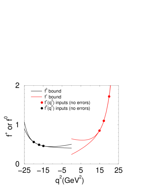
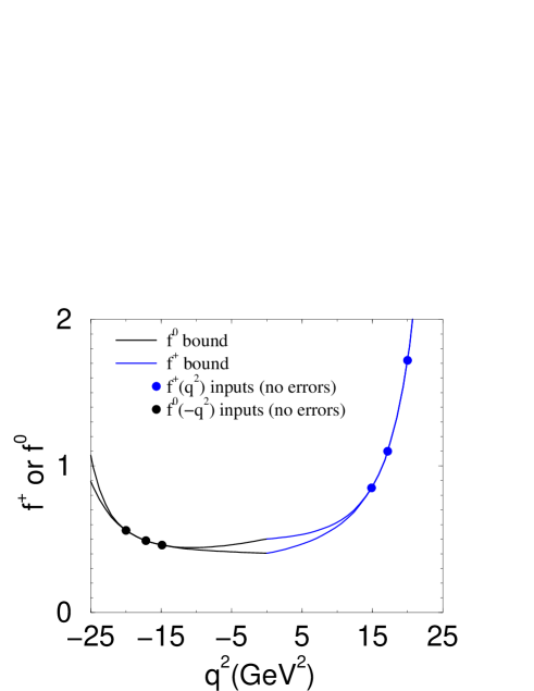
Figure 1: bound of $f^{+}(t),f^{0}(-t)$ for one example set of inputs $f$

The top figure shows the independent bounds for $F^{0}_{up/lo}$ and $F^{+}_{up/lo}$ and the bottom figure shows the bounds with the kinematical constraint $f^{+}(0)=f^{0}(0)$

Fig. 1 shows a typical shape of the dispersive bound using a mock data and it is suggested that the inputs at three points could give rather stringent constraints.

One problem is that in practice the additional inputs from the lattice calculation always has some theoretical errors so that this bound has uncertainties. Lellouch proposed a statistical treatment and derived a probability distribution the dispersive bound  Lellouch:1995yv . He made a random sample set of form factors which obey the Gaussian distributions where the central value and the deviations are taken from the central values and the error of the lattice data. For each sample set, the quadratic equations which determine the upper and lower bounds are solved. He imposed the following condition,

Condition A

(consistency condition):

• The quadratic equations to determine the upper/lower bounds should have real solutions.

• The solutions of the upper/lower bounds should allow the kinematical condition $f^{+}(0)=f^{0}(0)$.

The sample is accepted when condition A is satisfied and discarded otherwise. Then he makes a distributions of the upper and lower bounds from only the accepted solution, which are conditional distributions.

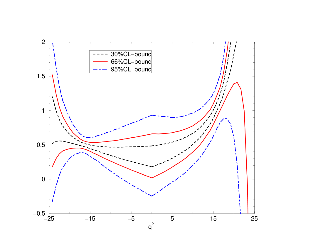
Figure 2: The confidence level bound for $f^{+}(t)$, $f^{0}(-t)$. The input data is lattice data(Lellouch).

As shown in Fig. 2, the confidence level bound at $q^{2}\sim 0$ and $q^{2}=q^{2}_{max}$ has a huge spread. Although the dispersive bound method gives bounds at certain confidence levels, they are not strong enough to constrain the CKM matrix element $|V_{ub}|$ with high accuracy.

In the following we would like to consider how to make the best use of the experimental data and the theoretical results. The large width of the dispersive bound arises because the statistical bound was obtained at each $q^{2}$ without considering the correlation in $q^{2}$. However, as shown in Fig. 1, each sample of the dispersive bound from the Monte Carlo sample based on the lattice data gives a very stringent bound and the $q^{2}$ dependence can be obtained with, say, 10% accuracy. On the other hand, from CLEO experiment we also know the $q^{2}$ dependence up to an overall normalization from unknown factor $|V_{ub}|$. The knowledge of the $q^{2}$ dependence of the form factors from both the theory and experiment can be an additional input for the determination of $|V_{ub}|$. To extract $|V_{ub}|$, instead of combining the experimental data and the lattice results for a single $q^{2}$ bin, we make a kind of simultaneous fit for all the $q^{2}$ bins. Precisely speaking, since the lattice results are transformed into the distributions of the upper and lower bounds, a little modifications are necessary, namely rather than fitting $|V_{ub}|$ we obtain a conditional distributions of $|V_{ub}|$ using all information from the experimental and the lattice results. In other words, we can reweight the statistical distribution of the form factor bounds using the $q^{2}$ distribution from the experiment as an additional input, which we will explain more in detail in the next section.

We also note that the soft pion theorem can also be used for additional inputs. The soft pion predicts that the form factor near the zero pion recoil limit ($q^{2}\rightarrow q^{2}_{max}$), the form factor behaves as

$$f^{0}(q^{2}_{max}) \rightarrow \frac{f_{B}}{f_{\pi}}$$ (4)

$$f^{+}(q^{2}_{max}) \rightarrow \frac{gf_{B^{*}}}{f_{\pi}}\frac{1}{1-q^{2}/m_{B^{*}}^{2}},$$ (5)

where $g$ is the $B^{*}B\pi$ coupling and $f_{B}\sim f_{B^{*}}$ are the decay constants of $B$ and $B^{*}$ mesons Burdman:1993es . Therefore provided that $g$, $f_{B}$, $f_{B^{*}}$ are known, the soft pion relation can be used to gives additional inputs of the form factor at $q^{2}_{max}$ for the dispersive bounds.

III Method

In the previous section, we explained the basic idea for extracting the CKM element $|V_{ub}|$ by combing the lattice results, experimental data, and the dispersive bound. In this section we explain our method more in detail.

Due to limited statistics and limited energy resolution in $q^{2}$ etc, usually the whole kinematic range is divided into $N_{bin}$ bins ($q^{2}_{i}<q^{2}<q^{2}_{i+1},i=1,\cdots,N_{bin}$ ) and we only know the partial decay rates for those $q^{2}$ bins

$$\Gamma^{exp}_{i}\equiv\int_{q^{2}_{i}}^{q^{2}_{i+1}}dq^{2}\frac{d\Gamma}{dq^{2}}=\frac{G^{2}|V_{ub}|^{2}}{192\pi^{3}m_{B}^{3}}\int_{q^{2}_{0}}^{q^{2}_{1}}dq^{2}|f^{+}(q^{2})|^{2}\lambda(q^{2})^{3/2}.$$ (6)

This partial decay rates are indeed measured by CLEO collaboration Athar:2003yg .

By integrating the dispersive bounds of the form factor $F^{+}_{up/lo}(q^{2};\mbox{\boldmath$f$})$ , we can predict the upper and lower bounds of the partial decay rate over certain $q^{2}$ bins up to the overall factor $|V_{ub}|^{2}$.

$$\gamma^{up/lo}_{i}(\mbox{\boldmath$f$})$$ (7)

$$\equiv \frac{G^{2}}{192\pi^{3}m_{B}^{3}}\int^{t_{i+1}}_{t_{i}}dt\left|F^{+}_{up/lo}(t;\mbox{\boldmath$f$}^{+},\mbox{\boldmath$f$}^{0})\right|^{2}\lambda(t)^{3/2},$$

where the theoretical upper/lower bounds of the partial decay rates are $\Gamma^{up/lo}_{i}(\mbox{\boldmath$f$})=|V_{ub}|^{2}\times\gamma^{up/lo}_{i}(\mbox{\boldmath$f$})$ .

Let us now explain our methods, which is composed of five steps.

1. We generate samples of $f$ from the Gaussian distribution with central values and errors from the lattice data. The samples of $B^{*}B\pi$ coupling $g$ and $f_{B}\sim f_{B^{*}}$ are also generated from the some distributions based on the best knowledge of $g$ and $f_{B}$, from which the samples of $\mbox{\boldmath$f$}_{max}\equiv\{f^{+}(q^{2}_{max}),f^{0}(q^{2}_{max})\}$ are produced. They can be used as additional data of the form factor for the dispersive bounds.

2. From each sample of $\{\mbox{\boldmath$f$},\mbox{\boldmath$f$}_{max}\}$, the dispersive bounds $F^{+}_{up/lo}(q^{2};\mbox{\boldmath$f$},\mbox{\boldmath$f$}_{max})$ (and $F^{0}_{up/lo}(q^{2};\mbox{\boldmath$f$},\mbox{\boldmath$f$}_{max})$) are derived and each sample is accepted or rejected under the Condition A, so that a conditional distribution is produced.

3. For each accepted sample, we compute the upper and lower bounds of the partial decay rate $\gamma^{up/lo}_{i}(\mbox{\boldmath$f$},\mbox{\boldmath$f$}_{max})$’s for a given set of $q^{2}$ bins.

4. We create samples of $|V_{ub}|$ and $\Gamma^{exp}_{i}$’s. We assume $|V_{ub}|$ distributes uniformly within a conservatively wide range, i.e. $|V_{ub}|=[1\times 10^{-3},6\times 10^{-3}]$. and $\Gamma^{exp}_{i}$’s are distributed by a Gaussian around their central values with variances given by the CLEO data.

5. We further impose the following physical condition for the set of samples $\{\mbox{\boldmath$f$},g,f_{B},|V_{ub}|,\Gamma^{exp}_{i}\}_{CondA}$.

   Condition B

   (physical condition):

   • The experimental data $\Gamma^{exp}_{i}$’s should lie within the upper and lower bounds from the theory simultaneously for all $i$ , i.e.
     $|V_{ub}|^{2}\gamma^{lo}_{i}<\Gamma^{exp}_{i}<|V_{ub}|^{2}\gamma^{up}_{i}$ (i=$1,\cdots,N_{bin}$).

   Try this test for all samples, select only those combinations which satisfies the condition B and reject others. This makes another conditional distribution of the set of samples $\{\mbox{\boldmath$f$},g,f_{B},|V_{ub}|,\Gamma^{exp}_{i}\}_{CondAB}$ which satisfies both Condition A and B.

Mathematically the original probability for the set of samples $\{\mbox{\boldmath$f$},g,f_{B},|V_{ub}|,\mbox{\boldmath$\Gamma$}^{exp}\}$ is given by the following product

$$P(\mbox{\boldmath$f$},g,f_{B},|V_{ub}|,\mbox{\boldmath$\Gamma$}^{exp})$$ (8)

$$= N\mathcal{P}_{\mbox{\boldmath$f$}}(\mbox{\boldmath$f$})\mathcal{P}_{g}(g)\mathcal{P}_{f_{B}}(f_{B})\mathcal{P}_{exp}(\mbox{\boldmath$\Gamma$}^{exp})\mathcal{P}_{|V_{ub}|}(|V_{ub}|),$$

where N is the normalization constant. The probability $\mathcal{P}_{\mbox{\boldmath$f$}},\mathcal{P}_{f_{B}},\mathcal{P}_{exp}$ are Gaussian distributions based on theoretical or experimental data, where as $\mathcal{P}_{g},\mathcal{P}_{|V_{ub}|}$ are uniform distributions.

After imposing the Condition A, the probability becomes

$$P_{A}(\mbox{\boldmath$f$},g,f_{B},|V_{ub}|,\mbox{\boldmath$\Gamma$}^{exp})$$ (11)

$$= \left\{\begin{array}[]{@{\,}ll}N^{\prime}P(\mbox{\boldmath$f$},g,f_{B},|V_{ub}|,\mbox{\boldmath$\Gamma$}^{exp})&\mbox{(if Cond A is satisfied), }\\ 0&\mbox{(otherwise),}\end{array}\right.$$

where $N^{\prime}$ is another normalization constant to make the total probability unity. By further imposing the Condition B, the probability then becomes

$$P_{AB}(\mbox{\boldmath$f$},g,f_{B},|V_{ub}|,\mbox{\boldmath$\Gamma$}^{exp})$$ (14)

$$= \left\{\begin{array}[]{@{\,}ll}N^{\prime\prime}P(\mbox{\boldmath$f$},g,f_{B},|V_{ub}|,\mbox{\boldmath$\Gamma$}^{exp})&\mbox{(if Cond A+B is satisfied),}\\ 0&\mbox{(otherwise),}\end{array}\right.$$

where $N^{\prime\prime}$ is another normalization constant.

Using this last conditional distribution $P_{AB}$, the distributions of any quantities defined from the set of samples $\{\mbox{\boldmath$f$},g,f_{B},|V_{ub}|,\mbox{\boldmath$\Gamma$}^{exp}\}_{AB}$, can be derived, which of course includes that of $|V_{ub}|$.

IV Results

IV.1 The setup

In this section we explain our results based on the lattice results and experimental data. The experimental data are taken from the results from CLEO collaboration Athar:2003yg . Table 1 shows the partial branching fraction $\Gamma_{i}/\Gamma_{total}$.

$q^{2}$bin	$[(\int d\Gamma/dq^{2})*dq^{2}]/\Gamma_{total}$
$0\leq q^{2}\leq 8GeV^{2}$	$(0.43\pm 0.11)\times 10^{-4}$
$8GeV^{2}\leq q^{2}\leq 16GeV^{2}$	$(0.65\pm 0.11)\times 10^{-4}$
$16GeV\leq q^{2}\leq q^{2}_{max}$	$(0.25\pm 0.09)\times 10^{-4}$

Table 1: CLEO data of partial branching ratio for $B\rightarrow\pi l\nu$

In order to convert $\Gamma_{i}$ we take $\Gamma_{total}=[4.29\pm 0.04]\times 10^{-13}GeV$  ref:PDG . There are lattice calculations from four different lattice groups in the quenched approximation Bowler:1999xn ; Abada:2000ty ; El-Khadra:2001rv ; Aoki:2001rd . In this section, we take the lattice result from JLQCD collaboration Aoki:2001rd . We picked the form factor data at three points of $q^{2}$’s for our analysis, which are listed in Table 2.

$q^{2}(GeV^{2})$	$f^{+}(q^{2})$	$f^{0}(q^{2})$
$17.79$	$1.03\pm 0.22$	$0.407\pm 0.092$
$19.30$	$1.24\pm 0.21$	$0.45\pm 0.11$
$20.82$	$1.54\pm 0.27$	$0.51\pm 0.14$

Table 2: lattice results of $f^{+}(q^{2})$ and $f^{0}(q^{2})$ by JLQCD

The recent $B^{*}B\pi$ coupling $g$ in quenched lattice QCD gives $g=0.48\pm 0.03\pm 0.11$ for the static limit and $g=0.58\pm 0.06\pm 0.10$ for the b quark from the quenched lattice calculations Abada:2003un . The QCD sum rule gives $g=0.36\pm 0.10$  Khodjamirian:1999hb . The predictions from quark models are in the range $0.3<g<0.8$ quark_models . In our analysis we took uniform distribution $g=[0.3,0.9]$. The decay constant $f_{B}$ is known with 30% error. Since this error is much larger than the splitting of $f_{B^{*}}$ and $f_{B}$, we took $f_{B^{*}}=f_{B}=190\pm 30$ MeV for simplicity, taking the best estimate by the lattice calculation Kronfeld:2003sd ; Aoki:2003xb .

In step 1 and 4, based on the above information we generated ${\cal O}(10^{7})$ set of samples for $\{\mbox{\boldmath$f$},g,f_{B}\}$ , 2,000 set of samples for $\{\mbox{\boldmath$\Gamma$}^{exp}\}$, and 2,000 samples for $|V_{ub}|$.

Imposing the condition A in step 2, 2000 set of samples of $\{\mbox{\boldmath$f$},g,f_{B}\}$ survives. In Fig. 3, the histogram for the samples of $f$ is shown. We find that the dispersive bound actually reduces the variance of the lattice data significantly.

Figure 3: distribution of form factor $f^{+}(q^{2}=17.79GeV^{2})$. The Top figure is the original samples from Gaussian distribution and the bottom is the samples which survived condition A.

In step 3, we compute the upper/lower bounds for the partial decay rate divided by $|V_{ub}|^{2}$ for each $q^{2}$ bins. To illustrate how it works, we pick up 3 generic set of samples ( samples 1, 2 and 3 ). In Fig. 4 we show the upper/lower bounds of the form factors for each sample. It should be noted the open window for each sample from $F^{+}_{up/lo}(q^{2})$ is very small.

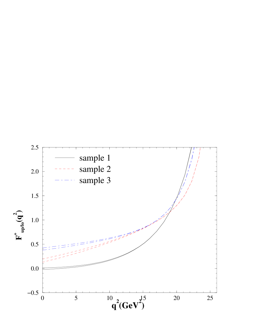
Figure 4: Upper/lower bounds of the form factors $f^{+}$ for sample 1, 2, 3.

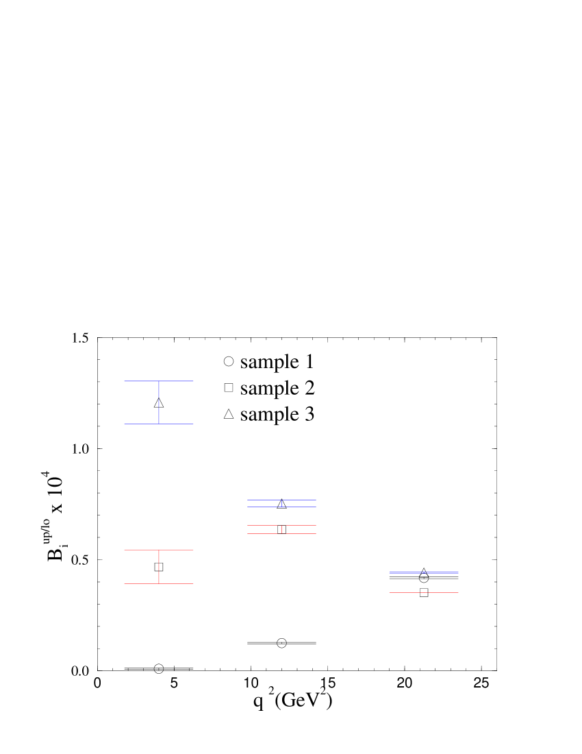
Figure 5: Upper/lower bounds of the partial branching fraction over the three energy bins for sample 1, 2, 3, where $B_{i}^{up/lo}\equiv\gamma_{i}^{up/lo}|V_{ub}|^{2}/\Gamma_{total}$. While the overall normalization is unknown up to $|V_{ub}|$, we have set $|V_{ub}|=3.71\times 10^{-3}$ for illustration.

Integrating the squares of these upper/lower bounds for the form factors for each sample, we obtain the upper/lower bounds for $\gamma^{up/lo}_{i}$ and the partial branching fraction $B_{i}^{up/lo}\equiv\gamma_{i}^{up/lo}|V_{ub}|^{2}/\Gamma_{total}$ for each $q^{2}$ bin as shown in Fig. 5. For comparison we also show the the partial branching fraction by CLEO collaboration in Fig. 6.

Figure 6: The partial branching fraction $B_{i}$’s over the three energy bins from CLEO, where $B_{i}\equiv\Gamma_{i}/\Gamma_{total}$.

In step 5, we impose condition B. As can be seen from Fig. 5 and Fig. 6, it is expected that the conditional probability with condition A+B would be highly suppressed for samples 1 and 3 but not so suppressed for sample 2.

The histogram for the samples of $f$ after imposing condition B is shown in Fig. 7. We find that the condition B reduces the variance of the form factor distribution even further.

Figure 7: distribution of $f^{+}(q^{2}=17.79GeV^{2})$ from the samples which survived condition A and B .

In order to understand the mechanism of the reduction of the variance, we show show the scatter plot of $\gamma_{3}/\gamma_{2}$ vs $\gamma_{2}$ or $\gamma_{1}/\gamma_{2}$ vs $\gamma_{2}$ in Fig. 8 . We find that there are clear correlations.

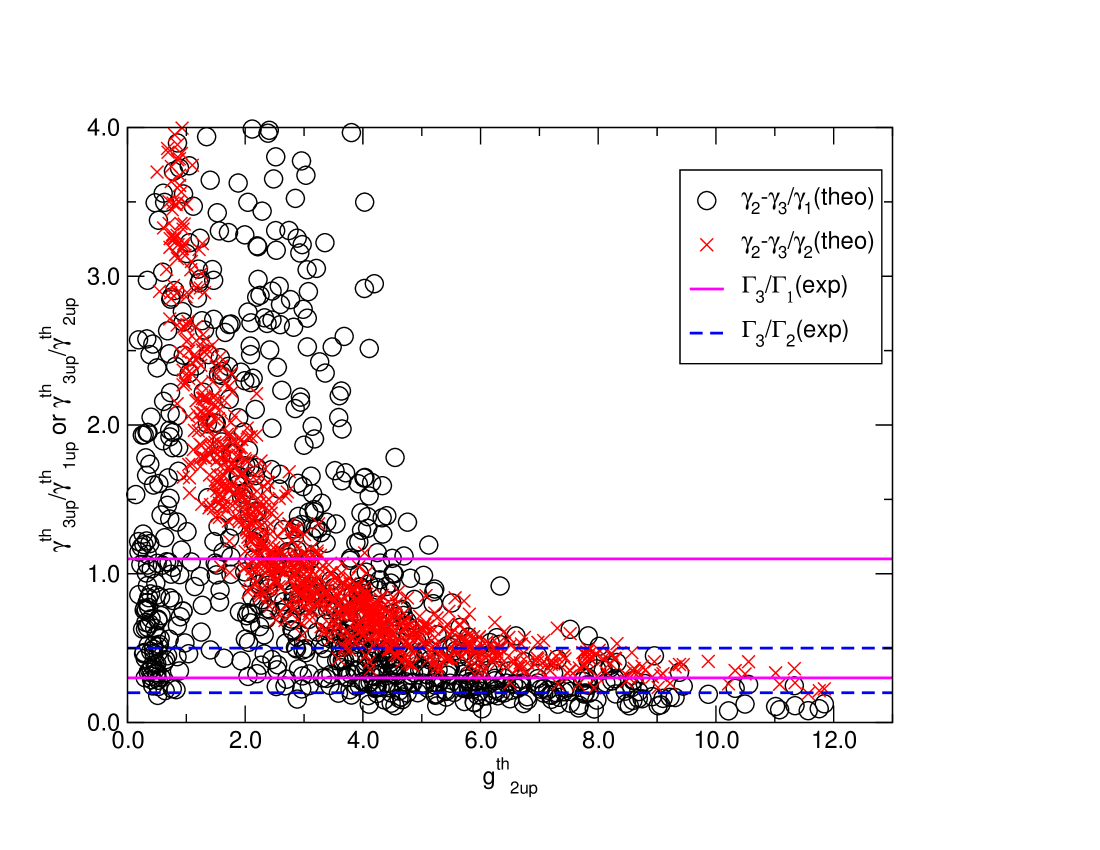
Figure 8: scatter plot of $\gamma^{th}_{3}/\gamma^{th}_{2}$ vs $\gamma^{th}_{2}$ and $\gamma^{th}_{1}/\gamma^{th}_{2}$ vs $\gamma^{th}_{2}$ under condition A. As a reference we also show the favored region of $\Gamma^{exp}_{3}/\Gamma^{exp}_{2}$ and $\Gamma^{exp}_{1}/\Gamma^{exp}_{2}$

From the CLEO data in Fig. 6, it can be shown that the experimental data favors the range $\Gamma^{exp}_{3}/\Gamma^{exp}_{2}\sim 0.2-0.5$ and $\Gamma^{exp}_{1}/\Gamma^{exp}_{2}\sim 0.4-0.9$.

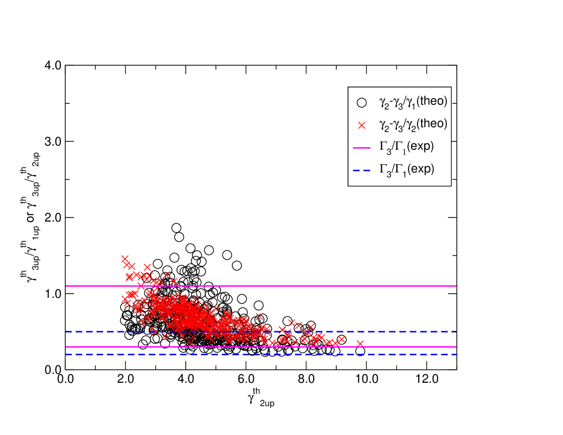
Figure 9: scatter plot of $\gamma^{th}_{3}/\gamma^{th}_{2}$ vs $\gamma^{th}_{2}$ and $\gamma^{th}_{1}/\gamma^{th}_{2}$ vs $\gamma^{th}_{2}$ after imposing condition A+B. As a reference we also show the favored region of $\Gamma^{exp}_{3}/\Gamma^{exp}_{2}$ and $\Gamma^{exp}_{1}/\Gamma^{exp}_{2}$.

.

Since the open window of upper/lower bounds for each sample is quite small, imposing condition B is similar to restricting $\gamma_{3}/\gamma_{2}=0.2-0.5$ and $\gamma_{1}/\gamma_{2}=0.4-0.9$ in Fig. 8. Since there is a strong correlation this restricts $\gamma_{2}$. In fact after imposing condition B, the scatter plot corresponding to Fig. 8 looks as Fig. 9.

IV.2 results

We give our final results for various physical quantities by looking their distributions which can be extracted from the conditional distribution $P_{AB}$.

First, the dispersive bound is shown in Fig. 10.

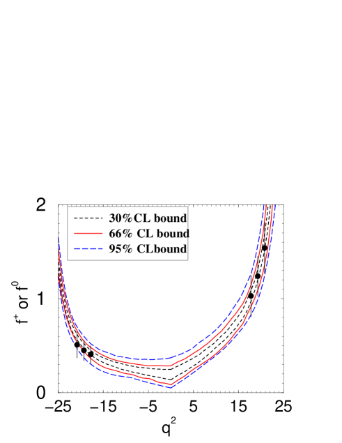
Figure 10: CLB for $f^{+}(q^{2})$. Here we used JLQCD’s lattice input, and CLEO’s experimental data.

Figure 11: Histograms of $|V_{ub}|$. The original distribution was assumed to be flat in the range $|V_{ub}|=[1,6]^{-3}$ (left). After imposing condition B, the resulting distribution distributes with small variance.

Fig. 11 shows the histogram of $|V_{ub}|$. From this distribution we obtain

$$|V_{ub}| = [3.73\pm 0.53]\times 10^{-3}.$$ (15)

This can be compared to the $|V_{ub}|$ determination using only the raw lattice data and the CLEO result at highest $q^{2}$ bin. For example, if we use the JLQCD results of the differential decay rate for $q^{2}>16$ GeV², we obtain $|V_{ub}|=[3.1\pm 0.9]\times 10^{-3}$. This means that the $|V_{ub}|$ error of 30% in the conventional method is reduced to 14 % in our new method.

This error reduction is rather remarkable and requires some explanation on which part of the analysis contributed most. One important ingredient is the condition A and the other important ingredient is the condition B. Also, whether or not we have a soft pion input is another important point. In order to see the effect of each ingredients, in addition to our full analysis we also carried out analyses with the following three cases.

1. Condition A only without soft pion input,

2. Condition A only and with soft pion input,

3. Condition A + B but without soft pion input.

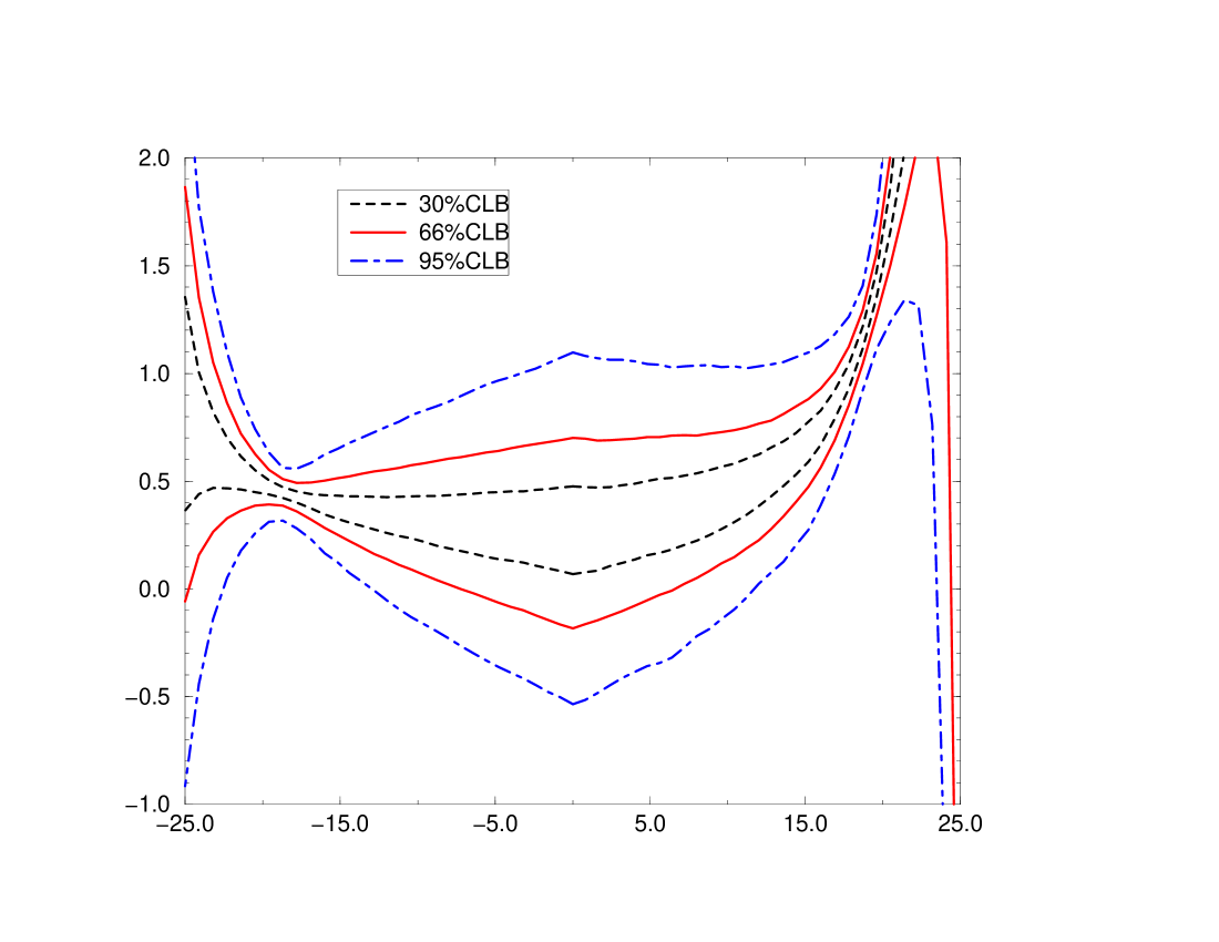
Figure 12: the case of Condition A only, without soft pion input.

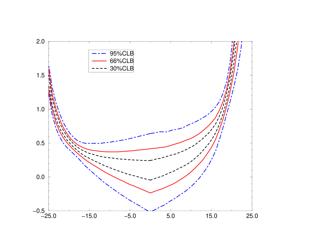
Figure 13: the case of Condition A only, with soft pion input.

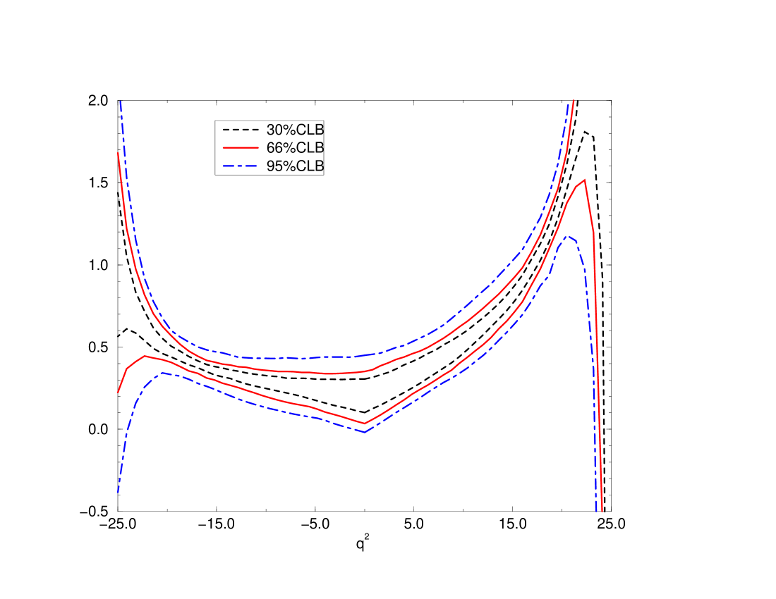
Figure 14: the case of Condition A+B, without soft pion input.

Fig. 12, Fig. 13, and Fig. 14 show the corresponding results.

The figures suggests that both condition A and condition B reduces the error. In fact, the corresponding $|V_{ub}|$ values are

$$|V_{ub}| = [2.92^{+0.65}_{-0.60}]\times 10^{-3}\mbox{ for case 1},$$ (16)

$$|V_{ub}| = [2.99^{+0.63}_{-0.49}]\times 10^{-3}\mbox{ for case 2},$$ (17)

$$|V_{ub}| = [3.61^{+0.55}_{-0.46}]\times 10^{-3}\mbox{ for case 3},$$ (18)

so that the error for $|V_{ub}|$ is has 20%, 20% and 14% for cases 1, 2 and 3 respectively. Thus we find both condition A and condition B reduces the error and having both of them together gives the significant reduction. It is also found that the input from the soft pion theorem does not change the result of $|V_{ub}|$ so much.

We also obtain product we also obtain bounds at 66% confidence level (66% CL) for $f^{+}(0)$ as a byproduct

$$0.126<f(0)<0.293.$$ (19)

which will be very useful for predicting the two body decay rate in QCD factorization .

V Systematic Errors

In this section we discuss possible systematic errors in our analysis.

The main systematic error arise from the lattice data and from the experimental data. These errors are of course already included in the errors of our input data. However, it would be nice if we could estimate these errors in a different fashion. One way to do so is to use the input data from other groups which has different systematic errors. In the following we present our result using different lattice inputs. Although we should also perform analyses using other experimental data such as those from Belle or BaBar, this will be left as a future problem since there is no publicly available data. Therefore we will not discuss the systematic errors from experimental data in this paper.

There are four quenched lattice calculations with different systematic errors. JLQCD collaboration used nonrelativistic effective theory for the heavy quark on a coarse lattice, in which the dominant systematic errors are the momentum dependent discretization error and chiral extrapolation error. Fermilab collaboration also used a different type of nonrelativistic effective theory on relatively coarse lattices, using different chiral extrapolation method. APE collaboration and UKQCD collaboration used relativistic action for the heavy quark on finer lattices, in which the dominant error is the presumably momentum independent discretization error from the large heavy quark mass in lattice units. In Table 3, we give the input parameters from APE, UKQCD and Fermilab collaborations.

collaboration	$q^{2}(GeV^{2})$	$f^{+}(q^{2})$	$f^{0}(q^{2})$
Fermilab	$17.23$	$1.13^{+0.29}_{-0.19}$	$0.64^{+0.13}_{-0.10}$
	$20.35$	$1.72^{+0.31}_{-0.27}$	$0.83^{+0.16}_{-0.13}$
	$23.41$	$2.10^{+0.43}_{-0.40}$	$1.00^{+0.20}_{-0.15}$
APE	$13.6$	$0.70^{+0.13}_{-0.09}$	$0.46^{+0.09}_{-0.11}$
	$17.9$	$1.05^{+0.15}_{-0.13}$	$0.59^{+0.07}_{-0.11}$
	$22.1$	$1.96^{+0.24}_{-0.30}$	$0.80^{+0.06}_{-0.13}$
UKQCD	$16.7$	$0.90\pm 0.22$	$0.57^{+0.06}_{-0.11}$
	$18.1$	$1.10^{+0.28}_{-0.22}$	$0.61^{+0.06}_{-0.11}$
	$22.3$	$2.30^{+0.67}_{-0.36}$	$0.79^{+0.05}_{-0.11}$

Table 3: lattice results of $f^{+}(q^{2})$ and $f^{0}(q^{2})$ by Fermilab, APE and UKQCD.

The setups for the numerical analysis are almost the same except for the number of generated samples for $\{\mbox{\boldmath$f$},g,f_{B}\}$ in step 1. In the analyses using Fermilab, APE and UKQCD data, we have generated ${\cal O}(10^{5})$ samples. The results using Fermilab data are

$$|V_{ub}|=[3.59^{+0.42}_{-0.40}]\times 10^{-3},$$ (20)

$$0.128<f(0)<0.339\mbox{ (at 66\% CL)},$$ (21)

those using APE data are

$$|V_{ub}|=[3.35^{+0.45}_{-0.49}]\times 10^{-3},$$ (22)

$$0.132<f(0)<0.302\mbox{ (at 66\% CL)},$$ (23)

those using UKQCD data are

$$|V_{ub}|=[3.37^{+0.46}_{-0.49}]\times 10^{-3},$$ (24)

$$0.154<f(0)<0.353\mbox{ (at 66\% CL)}.$$ (25)

Another possible source of systematic errors are the theoretical input values of $\chi_{L}(0)$, $\chi_{T}(0)$ for the dispersive bound which is obtained by the operator product expansion (OPE) using perturbative QCD and some estimate of vacuum condensation values. (See appendix for more details.) As is explained in the appendix these input values are

$$\chi_{T} = [5.60\pm 0.17]\times 10^{-4},$$ (26)

$$\chi_{L} = [1.50\pm 0.03]\times 10^{-2},$$ (27)

where the errors are from unknown 2-loop perturbative corrections and uncertainties in the vacuum condensation values. By changing the input values of $\chi_{T}$ and $\chi_{L}$ by 1 $\sigma$, the central values of $|V_{ub}|$ changes by 2% when JLQCD data are used, which is negligible compared to other errors. We also found that the same is true when Fermilab, APE, or UKQCD data are used.

Yet another systematic error is the quenching error in the lattice results. Since there is no way to control this error other than performing unquenched lattice calculations, which is beyond the scope of this paper. We leave it an open question and wait for the unquenched lattice results, which is expected to appear near future.

VI Conclusion

In this paper, we have proposed a method to determine $|V_{ub}|$ by combining lattice results, dispersive bounds, and experimental data. Based on Lellouch’s idea we considered the statistical distributions of the form factors and their bounds. Our proposal is to restrict the distribution by imposing a physical condition using the experimental data. This gives a significant reduction in the errors of $|V_{ub}|$ . As as result we obtained

$$|V_{ub}| = [3.73\pm 0.53]\times 10^{-3}.$$ (28)

As a by product we also obtained a 66% confidence level bound for the form factor at small $q^{2}$,

$$0.293 <f(0)<0.126$$ (29)

which will be very useful for predicting the two body decay rate in QCD factorization.

The recent Belle results of $|V_{ub}|$ from $B\rightarrow X_{u}l\nu$  Kakuno:2003fk is

$$|V_{ub}|=[4.66\pm 0.28\pm 0.35\pm 0.17\pm 0.08\pm 0.58]\times 10^{-3},$$ (30)

where the errors is the statistical, systematic, $b\rightarrow c$, $b\rightarrow u$, and theoretical. The lattice QCD based $|V_{ub}|$ values by CLEO collaboration from $B\rightarrow\pi l\nu$ is

$$|V_{ub}| = [2.88\pm 0.55\pm 0.30{}^{+0.45}_{-0.35}\pm 0.18]\times 10^{-3},$$ (31)

where the errors are statistical, experimental systematic, theoretical and $\rho l\nu$ form factor shape. It should be noted that this discrepancies are reduced by our method although the input lattice data are the same.

For future studies, we should elaborate our method in such a way that we treat the systematic and statistical errors separately which would give a more careful analysis of errors. This is in principle straightforward but requires more numerical calculation since the generation of random samples should be much increased.

Another improvement is to update the input data of form factors from lattice, especially the unquenched one, and the input data of partial decay rates from B factories such as Belle and BaBar. Both of these will be available near future.

Appendix: Review of the Dispersive Bound

In this appendix, we briefly summarize the dispersive bounds on the form factors, which is fully discussed in Ref. Lellouch:1995yv . The matrix element of the heavy-to-light semileptonic decay $B\rightarrow\pi l\nu$ is parameterized as Eq. (1). The form factors $f^{+}$ and $f^{0}$ satisfies the following kinematical constraint

$$f^{+}(0)=f^{0}(0).$$ (32)

In order to derive bound on $f^{+}(q^{2})$ and $f^{0}(q^{2})$ we consider the following two-point function

$$\Pi^{\mu\nu}(q) \equiv i\int d^{4}x\rm{e}^{iqx}\langle 0\rvert TV^{\mu}(x)V^{\nu}(0)\lvert 0\rangle$$ (33)

$$= -(g^{\mu\nu}q^{2}-q^{\mu}q^{\nu})\Pi_{T}(q^{2})+q^{\mu}q^{\nu}\Pi_{L}(q^{2}),$$

where $\Pi_{T(L)}$ corresponds to the contribution from the intermediate states with $J^{P}=1^{-}(0^{+})$. In the deep Euclidean region which is far from the physical cut, this two point function can be evaluated by perturbative QCD reliably.

Inserting all possible intermediate states $|\Gamma\rangle$ we obtain the following result for the imaginary part of $\Pi_{\mu\nu}$:

$$-(g^{\mu\nu}q^{2}-q^{\mu}q^{\nu}){\rm Im}\Pi_{T}+q^{\mu}q^{\nu}{\rm Im}\Pi_{L}$$ (34)

$$= \frac{1}{2}\sum_{\Gamma}(2\pi)^{4}\delta^{4}(q-p_{\Gamma})\langle 0\rvert V^{\mu}\lvert\Gamma\rangle\langle\Gamma\rvert V^{\nu^{\dagger}}\lvert 0\rangle,$$

We now restrict ourselves to include only contributions of the $B\pi$ and the $B^{*}$ states. Since each hadron state contributes positively to the spectral function, we derive the following two bounds for the form factors

$${\rm Im}\Pi_{L}(t) \geq \frac{3t_{+}t_{-}}{32\pi}\sqrt{(t-t_{+})(t-t_{-})}\frac{|f^{0}(t)|^{2}}{t^{3}}\theta(t-t_{+}),$$

$${\rm Im}\Pi_{T}(t) \geq \pi\left(\frac{m_{B^{*}}}{f_{B^{*}}}\right)^{2}\delta(t-{m_{B^{*}}}^{2})$$

$$+\frac{1}{32\pi}\frac{[(t-t_{+})(t-t_{-})]^{3/2}}{t^{3}}|f^{+}(t)|^{2}\theta(t-t_{+}),$$

where $t\equiv q^{2}$ and $t_{\pm}\equiv(m_{B}\pm m_{\pi})^{2}$ . In the above equations we have limited ourselves to contribution of the $B^{*}$ state with

$$\langle 0\rvert V^{\mu}\lvert B^{*}(r,p)\rangle=\frac{m_{B^{*}}^{2}}{f_{B^{*}}}\epsilon^{\mu}_{r}$$ (35)

In QCD, the polarization functions $\Pi_{L}$ and $\Pi_{T}$ obey once and twice subtracted dispersion relation($q^{2}=-Q^{2}$), i.e.:

$$\chi_{L}(Q^{2}) \equiv -\frac{\partial}{\partial Q^{2}}(-Q^{2}\Pi_{L}(Q^{2}))$$ (36)

$$= \int^{\infty}_{0}\frac{dt}{\pi}\frac{t{\rm Im}\Pi_{L}(t)}{(t+Q^{2})^{2}}$$

$$\chi_{T}(Q^{2}) \equiv \frac{1}{2}\left(-\frac{\partial}{\partial Q^{2}}\right)^{2}(-Q^{2}\Pi_{T}(Q^{2}))$$ (37)

$$=\int^{\infty}_{0}\frac{dt}{\pi}\frac{t{\rm Im}\Pi_{T}(t)}{(t+Q^{2})^{3}}$$

Thus it is now possible to get bounds on the form factors to inserts Eqs.(36,37) to Eqs.(Appendix: Review of the Dispersive Bound,Appendix: Review of the Dispersive Bound)

$$J_{L}(Q^{2}) \geq \frac{1}{\pi}\int_{t_{+}}^{\infty}dtk_{L}(t,Q^{2})|f_{0}(t)|^{2}$$ (38)

$$J_{T}(Q^{2}) \geq \frac{1}{\pi}\int_{t_{+}}^{\infty}dtk_{T}(t,Q^{2})|f_{+}(t)|^{2}$$ (39)

where $J_{L(T)},k_{L(T)}$ are

$$J_{L} = \chi_{L}(Q^{2}),$$ (40)

$$J_{T} = \chi_{T}(Q^{2})-\frac{1}{(m_{B^{*}}+Q^{2})^{3}}\left(\frac{m_{B^{*}}^{2}}{f_{B^{*}}}\right)^{2},$$ (41)

$$k_{L} = \frac{3}{32\pi}\frac{[(t-t_{+})(t-t_{-})]^{1/2}t_{+}t_{-}}{(t+Q^{2})^{2}t^{2}},$$ (42)

$$k_{T} = \frac{3}{96\pi}\frac{[(t-t_{+})(t-t_{-})]^{3/2}}{(t+Q^{2})t^{2}}.$$ (43)

To obtain the bounds of the form factor for values of t in the range $[0,t_{-}]$, we map the complex t-plane into the unit disc in complex z-plane with the conformal transformation

$$\frac{1+z}{1-z}=\sqrt{\frac{(t_{+}-t)(t_{-}-t)}{t_{+}-t_{-}}}.$$

This maps the contour along the physical cut in Eqs.(38,39) onto a unit circle in z-plane so that

$$J_{L}(Q^{2}) \geq \oint_{c}\frac{dz}{2\pi iz}|\phi_{L}(z,Q^{2})f_{0}(z)|^{2},$$ (44)

$$J_{T}(Q^{2}) \geq \oint_{c}\frac{dz}{2\pi iz}|\phi_{T}(z,Q^{2})f_{+}(z)|^{2},$$ (45)

where we have used the fact that $k(t,Q^{2})$ is positive definite quantity. The functions $\phi_{L(T)}$ are defined as

$$\phi_{L} = \sqrt{\frac{3t_{+}t_{-}}{4\pi}}\frac{1}{t_{+}-t_{-}}\frac{1+z}{(1-z)^{5/2}}\left(\sqrt{\frac{t_{+}}{t_{+}-t_{-}}}+\frac{1+z}{1-z}\right)^{-2}$$

$$\left(\sqrt{\frac{t_{+}-Q^{2}}{t_{+}-t_{-}}}+\frac{1+z}{1-z}\right)^{-2},$$

$$\phi_{T} = \sqrt{\frac{1}{\pi(t_{+}-t_{-})}}\frac{(1+z)^{2}}{(1-z)^{9/2}}\left(\sqrt{\frac{t_{+}}{t_{+}-t_{-}}}+\frac{1+z}{1-z}\right)^{-2}$$

$$\left(\sqrt{\frac{t_{+}-Q^{2}}{t_{+}-t_{-}}}+\frac{1+z}{1-z}\right)^{-3},$$

and satisfy $\phi(z,Q^{2})\geq 0$ for $t\in[0,t^{-}]$. For simplicity, we define an inner product on the unit circle

$$\langle g|h\rangle=\oint_{|z|=1}\frac{dz}{2\pi iz}g^{*}(z)h(z),$$ (46)

so that the inequality Eq. (44), Eq. (45) can be written

$$J\geq\langle\phi f|\phi f\rangle.$$ (47)

And define the function $g_{t}(z)$ and the matrix $M(f(t))$ as

$$g_{t}(z) \equiv \frac{1}{1-z^{*}(t)z},$$

$$M(f(t)) = \begin{pmatrix}\langle\phi f|\phi f\rangle&\langle\phi f|g_{t}\rangle\\ \langle g_{t}|\phi f\rangle&\langle g_{t}|g_{t}\rangle,\end{pmatrix}$$

then if $f(z(t))$ has no pole in the range $[0,t_{-}]$, $f(z(t))$ can be related the inner-product of $g_{t}$ and $\phi f$ as

$$\langle g_{t}|\phi f\rangle=\phi(z(t),Q^{2})f(z(t))$$ (48)

Now, because positivity of inner products

$$\det M(f(t),f(t_{1}))\geq 0$$ (49)

is satisfied, by eliminating $\langle\phi f|\phi f\rangle$ with (44,45) we get the form factors bound as

$$|f(t)|^{2}\leq J(Q^{2})\frac{1}{1-|z(t)|^{2}}\frac{1}{\phi(z(t),Q^{2})}.$$ (50)

If we want to get more conditionality bound, using some values of the form factors at $t_{1},t_{2},\cdots,t_{L}$ and defining the matrix $M(f(t),\mbox{\boldmath$f$})$ as

$$M(f(t),\mbox{\boldmath$f$})=\begin{pmatrix}\langle\phi f|\phi f\rangle&\langle\phi f|g_{t}\rangle&\langle\phi f|g_{t_{3}}\rangle&\cdots&\langle\phi f|g_{t_{N}}\rangle\\ \langle g_{t}|\phi f\rangle&\langle g_{t}|g_{t}\rangle&\langle g_{t}|g_{t_{3}}\rangle&\cdots&\langle g_{t}|g_{t_{N}}\rangle\\ \langle g_{t_{3}}|\phi f\rangle&\langle g_{t_{3}}|g_{t}\rangle&\langle g_{t_{3}}|g_{t_{3}}\rangle&\cdots&\langle g_{t_{3}}|g_{t_{N}}\rangle\\ \vdots&\vdots&\vdots&\vdots&\vdots\\ \langle g_{t_{N}}|\phi f\rangle&\langle g_{t_{N}}|g_{t}\rangle&\langle g_{t_{N}}|g_{t_{3}}\rangle&\cdots&\langle g_{t_{N}}|g_{t_{N}}\rangle\end{pmatrix},$$ (51)

where $f$ stand for $\{f(z(t_{1})),f(z(t_{2})),\cdots,f(z(t_{L}))\}$. This matrix $M(f(t),\mbox{\boldmath$f$})$ satisfies

$$detM(f(t),\mbox{\boldmath$f$})\geq 0,$$

By eliminating $\langle\phi f|\phi f\rangle$ using (44,45), the inequality (Appendix: Review of the Dispersive Bound) leads to bounds on the form factors $f(t)$,

$$F_{lo}(t;\mbox{\boldmath$f$})\leq f(t)\leq F_{up}(t;\mbox{\boldmath$f$}).$$

This upper and lower functions $F_{up(lo)}$ stand for

$$F_{up/lo}=\frac{-\beta(t)+/-\sqrt{c(Q^{2})\cdot\Delta(t)}}{\alpha\cdot\phi(t,Q^{2})},$$ (52)

where $\alpha$, $\beta(t)$, and $\sqrt{c(Q^{2})\cdot\Delta(t)}$ are known functions of $Q^{2}$, $t_{i}$, and $f(z(t_{i}))$ ($i=1,\cdots,L$). The particular form of the Eqs. (52) can be found in Ref. Lellouch:1995yv .

Now, if $f_{+}(t)$ has a single pole at $t=t_{p}$ away from the cut (in fact $t_{p}=m_{B^{*}}\in[t_{-},t_{+}]$), Eqs. (48) becomes

$$\langle g_{t}|\phi f\rangle=\phi(z(t))f(z(t))+\frac{Res(\phi f;z(t_{p}))}{z(t_{p})-z(t)}$$

so $\langle g_{t}|\phi f\rangle$ have the single pole at $z=z(t_{p})$. In this case we define the function $\phi_{p}(z)$, which satisfies $|\phi_{p}|=|\phi|$ at $|z|=1$, as,

$$\phi_{p}(z,Q^{2})\equiv\phi(z,Q^{2})\frac{z-z(t_{p})}{1-z^{*}(t_{p})z}.$$

This function $\phi_{p}f_{p}$ dose not have a pole at $z=z(t_{p})$, so

$$\langle\phi_{p}f_{p}|g_{t}\rangle = \phi_{p}(t)f_{p}(t)$$

$$\langle\phi_{p}f_{p}|\phi_{p}f_{p}\rangle = \langle\phi f|\phi f\rangle\leq J(Q^{2})$$

are satisfied. Thus, the bound of Eqs. (52)holds

$$F_{lo}^{p}(t;\mbox{\boldmath$f$})\leq f(t)\leq F_{up}^{p}(t;\mbox{\boldmath$f$}).$$

where $F_{lo,up}^{p}$ are the functions $F_{lo,up}$ obtained by replacing $\phi$ with $\phi_{p}$ . In this paper we denote $\phi_{p},F_{lo,up}^{p}$ as $\phi,F_{lo,up}$ for $f^{+}$. In this way, we get the the independent bounds on the form factors using the given values of the discrete set of points ,for example top figure of Fig. 1 with no kinematical constraint. But form factors not independent but satisfy the kinematical constraint Eqs.32. So we make a new dispersive bound, use

$$f^{+}(0)_{up}=F_{up}^{0}(0,\mbox{\boldmath$f$})$$ (53)

as the additional input of the new bound for $f^{+}(t)$, and consider this upper bound as new appear bound for $f^{+}(t)$. And equally make a new lower bound for $f^{+}(t)$, using the additional input

$$f^{+}(0)_{lo}=F_{lo}^{+}(0,\mbox{\boldmath$f$}).$$ (54)

So we can make kinematical constraint dispersive bound like bottoms of fig1. There may exist 4 pattern no kinematical constraint bound, from there kinematical constraint bound can be made respectively same method.

In this calculation, they use OPE and calculate the coefficient by perturbative QCD. In this paper, we take $\chi_{T}(0)=(5.60\pm 0.17)\times 10^{-4},\chi_{L}(0)=(1.50\pm 0.03)\times 10^{-2}$ (See Ref. Lellouch:1995yv ). The values of $\chi$ in $\overline{MS}$ scheme are given in Table. 4. These coefficients are obtained from the operator product expansion of hadron current correlators in perturbative approximation. In order to control the higher order contributions which grow for larger $-Q^{2}$, we take $Q^{2}=0$. The table shows that the $O(\alpha_{s})/1Loop$ are 17%,7% for $\chi_{T},\chi_{L}$ so that the perturbative expansion is under control. The unknown 2-loop errors can be estimated by either naive order counting or by comparing results with different renormalization schemes, which amount to less than or equal to 1%. We therefore estimate the uncertainties in $\chi$ from the condensates, which are of order 2% and 3% for $\chi_{L}$ and $\chi_{T}$.

	$\chi_{L}(Q^{2}=0)$	$\chi_{T}(Q^{2}=0)$
$1Loop$	$1.3\times 10^{-2}$	$5.1\times 10^{-4}$
$O(\alpha_{s})/1Loop$	$17\%$	$7\%$
total pert	$1.5\times 10^{-2}$	$5.5\times 10^{-4}$
$m_{u}<\bar{u}u>/1Loop$	$-2\%$	$3\%$
$<\alpha_{s}G^{2}>/1Loop$	$0.04\%$	$-0.05\%$
$total$	$1.5\times 10^{-2}$	$5.6\times 10^{-4}$

Table 4: perturbative and non-perturbative contributions to subtracted polarization function $\chi_{L}$ and $\chi_{T}$ by $\bar{MS}$-scheme. “1 Loop” stands for the 1-loop result and “totalpart” stands for the results through $O(\alpha_{s})$. $m_{u}<\bar{u}u>/1loop$,$<\alpha_{s}G^{2}>$ are the higher twist contributions from the condensates.

References

• (1) C. W. Bauer, Z. Ligeti and M. E. Luke, Phys. Rev. D 64, 113004 (2001).
• (2) L. Lellouch, Nucl. Phys. B 479, 353 (1996).
• (3) S. B. Athar et al. [CLEO Collaboration], Phys. Rev. D 68, 072003 (2003).
• (4) Particle Data Group.
• (5) T. Mannel and B. Postler, Nucl. Phys. B 535, 372 (1998).
• (6) D. Becirevic, Phys. Lett. B 399, 163 (1997).
• (7) S. Okubo and I. F. Shih, Phys. Rev. D 4 (1971) 2020.
• (8) C. Bourrely, B. Machet and E. de Rafael, Nucl. Phys. B 189, 157 (1981).
• (9) C. G. Boyd, B. Grinstein and R. F. Lebed, Phys. Rev. Lett.  74, 4603 (1995).
• (10) E. de Rafael and J. Taron, Phys. Rev. D 50, 373 (1994).
• (11) H. Kakuno et al. [BELLE Collaboration], Phys. Rev. Lett.  92, 101801 (2004).
• (12) G. Burdman, Z. Ligeti, M. Neubert and Y. Nir, Phys. Rev. D 49, 2331 (1994).
• (13) A. Abada, D. Becirevic, P. Boucaud, G. Herdoiza, J. P. Leroy, A. Le Yaouanc and O. Pene, JHEP 0402, 016 (2004).
• (14) A. Khodjamirian, R. Ruckl, S. Weinzierl and O. I. Yakovlev, Phys. Lett. B 457, 245 (1999). quark_models
• (15) D. Melikhov and M. Beyer, Phys. Lett. B 452, 121 (1999); J. L. Goity and W. Roberts, Phys. Rev. D 64, 094007 (2001); M. Di Pierro and E. Eichten, Phys. Rev. D 64, 114004 (2001); W. Jaus, Phys. Rev. D 67, 094010 (2003).
• (16) A. S. Kronfeld, Nucl. Phys. Proc. Suppl.  129, 46 (2004) [arXiv:hep-lat/0310063].
• (17) S. Aoki et al. [JLQCD Collaboration], Phys. Rev. Lett.  91, 212001 (2003).
• (18) S. Aoki et al. [JLQCD Collaboration], Phys. Rev. D 64, 114505 (2001).
• (19) A. Abada, D. Becirevic, P. Boucaud, J. P. Leroy, V. Lubicz and F. Mescia, Nucl. Phys. B 619, 565 (2001).
• (20) A. X. El-Khadra, A. S. Kronfeld, P. B. Mackenzie, S. M. Ryan and J. N. Simone, Phys. Rev. D 64, 014502 (2001).
• (21) K. C. Bowler et al. [UKQCD Collaboration], Phys. Lett. B 486, 111 (2000).