Calorons with non-trivial holonomy on and off the lattice HU-EP-04/44, ITEP-LAT/2004-16

Abstract

We discuss recent solutions for SU(2) calorons with non-trivial holonomy at higher charge, both through analytic means and using cooling, as well as extensive lattice studies for SU(3).

1 Introduction

We first briefly summarize the essential features of instantons at finite temperature $T$, so-called calorons [1]. A non-trivial Polyakov loop at spatial infinity (the so-called holonomy), which in some sense plays the role of a Higgs field, reveals the monopole constituent nature of these calorons [2, 3, 4]. Trivial holonomy, i.e. with values in the center of the gauge group, is typical for the deconfined phase. Non-trivial holonomy is therefore expected to play a role in the confined phase ($T<T_{c}$) where the trace of the Polyakov loop fluctuates around zero. The properties of instantons are therefore coupled to the order parameter for the deconfining phase transition.

Finite action requires the Polyakov loop at spatial infinity to be constant which for SU($n$) can be parametrized by

$${{\cal P}_{\infty}}=g^{\dagger}\exp(2\pi i{\rm diag}(\mu_{1},\mu_{2},\ldots,\mu_{n}))g,$$ (1)

where $\sum_{m=1}^{n}\mu_{m}=0$ and $g$ is chosen to bring ${{\cal P}_{\infty}}$ to its diagonal form, with the $n$ eigenvalues being ordered as $\mu_{1}\leq\mu_{2}\leq\ldots\leq\mu_{n}\leq\mu_{n+1}\equiv 1+\mu_{1}$. Caloron solutions are such that the total magnetic charge vanishes. A single caloron with topological charge one contains $n\!-\!1$ monopoles with a unit magnetic charge in the $j$-th U(1) subgroup, which are compensated by the $n$-th monopole of so-called type $(1,1,\ldots,1)$, having a magnetic charge in each of these subgroups [5]. At topological charge $Q$ there are $|Q|n$ constituents, $|Q|$ monopoles of each of the $n$ types. The monopole of type $m$ has a mass $8\pi^{2}\nu_{m}/b$ and its core has a size $b/(4\pi\nu_{m})$, with $\nu_{m}\!\equiv\!\mu_{m\!+\!1}\!-\!\mu_{m}$. The sum rule $\sum_{m=1}^{n}\!\nu_{m}\!=\!1$ guarantees the correct action $8\pi^{2}|Q|$ for calorons with topological charge $Q$. We can use the classical scale invariance to set $b\!=\!1/kT$, the period in the imaginary time direction, to 1.

Perturbative fluctuations give rise to an effective potential as a function of the background Polyakov loop, whose minima occur where the latter takes values in the center of the gauge group [6]. Recently the non-perturbative contribution due to the calorons at non-trivial holonomy was calculated [7], and when added to the perturbative contribution, the minima at trivial holonomy turn unstable for decreasing temperature, right around the expected value of $T_{c}$. This lends some support to monopole constituents being the relevant degrees of freedom which drive the transition from a phase in which the center symmetry is broken at high temperatures to one in which the center symmetry is restored at low temperatures.

The charge one SU($n$) action density, ${\cal{S}}(x)=-{\scriptstyle{\frac{1}{2}}}{\rm Tr}F_{\mu\nu}^{2}(x)$, has a particularly simple form [5],

$$\hskip-17.07164pt{\rm Tr}F_{\mu\nu}^{\,2}(x)\!=\!\partial_{\mu}^{2}\partial_{\nu}^{2}\log\left[{\scriptstyle{\frac{1}{2}}}{\rm tr}({\cal{A}}_{n}\cdots{\cal{A}}_{1})-\cos(2\pi t)\right],$$

$$\hskip-17.07164pt{\cal{A}}_{m}\equiv\frac{1}{r_{m}}\Biggl{(}\!\!\!\begin{array}[]{cc}r_{m}\!\!&|\vec{y}_{m}\!\!-\!\vec{y}_{m+1}|\\ 0\!\!&r_{m+1}\end{array}\!\!\!\Biggr{)}\Biggl{(}\!\!\!\begin{array}[]{cc}c_{m}\!\!&s_{m}\\ s_{m}\!\!&c_{m}\end{array}\!\!\!\Biggr{)},$$ (6)

with $r_{m}\!=\!|\vec{x}\!-\!\vec{y}_{m}|$ the distance to the $m^{\rm th}$ constituent monopole at $\vec{y}_{m}$, $c_{m}\!\equiv\!\cosh(2\pi\nu_{m}r_{m})$, $s_{m}\!\equiv\!\sinh(2\pi\nu_{m}r_{m})$, $r_{n+1}\!\equiv\!r_{1}$ and $\vec{y}_{n+1}\!\equiv\!\vec{y}_{1}$. The chiral fermion zero mode is localized [8, 9] to the $m^{\rm th}$ constituent monopole, provided one uses $\mu_{m}\!<\!z\!<\!\mu_{m+1}$ for the boundary condition $\hat{\Psi}_{z}(t+1,\vec{x})\!=\exp(-2\pi iz)\hat{\Psi}_{z}(t,\vec{x})$. “Cycling” through the values of $z$ gives the distinct signature of “jumping” zero modes through which one can identify well-dissociated calorons, as observed in lattice studies for SU(2) [10] and SU(3) [11].

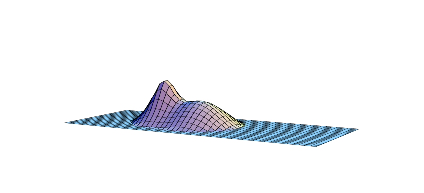
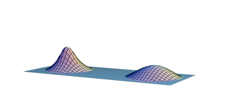
Figure 1: Two charge one SU(2) caloron profiles at $t\!=\!0$ with $b\!=\!1$ and $\mu_{2}\!=\!-\mu_{1}\!=\!0.125$, for $\rho\!=\!1.6$ (bottom) and 0.8 (top) on equal logarithmic scales (action density cutoff at $1/(2e^{2})$).

At any topological charge $Q$, well-separated constituents can be shown to act as point sources for the so-called far field, that is at large distance from any of the cores, where the gauge field is abelian [12]. When constituents of complementary charge ($n$ constituents of different type) come together, the action density no longer deviates significantly from that of a standard instanton. Its scale parameter $\rho$ is related to the constituent separation $d$ through $\pi\rho^{2}/b=d$. A typical example for a charge one SU(2) caloron with far and nearby constituents is shown in Fig. 1. When $\rho\ll b$ no difference would be seen with the action density of the Harrington-Shepard solution [1], the gauge field is nevertheless vastly different, as follows from the fact that within the confines of the peak there are $n$ locations where two of the eigenvalues of the Polyakov loop coincide [13, 14, 15]. When, on the other hand, constituents of equal charge come together (which requires $|Q|>1$) an extended core structure appears [12]. For two coinciding constituents this gives the typical doughnut structure also observed for monopoles [16], see Fig. 2.

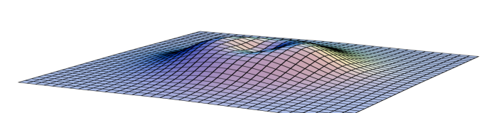
Figure 2: The action density (on a linear scale) of a typical SU(2) caloron with topological charge 2 and $\mu_{2}\!=\!-\mu_{1}\!=\!0.25$ for which two constituents of equal magnetic charge are closer than their individual sizes (but not exactly on top). The other two constituents are far away, for which this becomes a static charge two monopole solution.

2 Analytic SU(2) results at higher charge

Also at higher topological charge the zero modes, denoted by $\hat{\Psi}_{z}^{a}(x)$, where $a=1,\ldots,|Q|$, play an important role. We can write

$$\hat{\Psi}_{z}^{a}(x)^{\dagger}\hat{\Psi}_{z}^{b}(x)=-(2\pi)^{-2}\partial_{\mu}^{2}\hat{f}^{ab}_{x}(z,z).$$ (7)

where $\hat{f}^{ab}(z,z^{\prime})$ is a Green’s function that appears in the construction to be discussed below.

2.1 The far field limit

The trace, i.e. the sum over the zero-mode densities, has a remarkably simple form in the far field limit (denoted by ${\rm{ff}}$ and defined by neglecting terms that decay exponentially with the distance to any of the constituent cores)

$${\rm tr}\hat{f}^{\rm{ff}}_{x}(z,z)=4\pi^{2}{\cal{V}}_{m}(\vec{x}),\ \mbox{for}\ \mu_{m}<z<\mu_{m+1}.$$ (8)

As is implicit in the notation, ${\cal{V}}_{m}$ is static and independent of $z$ within its interval of definition. In addition ${\cal{V}}_{m}$ has to be harmonic (up to singularities), because the zero modes decay exponentially as long as $z\neq\mu_{j}$ (for any $j$), and therefore do not survive in the far field limit. For $Q=1$ one simply has ${\cal{V}}_{m}(\vec{x})=1/(4\pi|\vec{x}-\vec{y}_{m}|)$, whereas for $Q=2$ we found [12]

$${\cal{V}}_{m}(\vec{x})\!=\!\frac{1}{2\pi|\vec{x}|}+\frac{{\cal{D}}}{4\pi^{2}}\!\int_{r<{\cal{D}}}\hskip-14.22636ptdrd\varphi~{}\frac{\partial_{r}|\vec{x}-r\vec{y}(\varphi)|^{-1}}{\sqrt{{\cal{D}}^{2}-r^{2}}},$$ (9)

where $\vec{y}(\varphi)\!=\!(\sqrt{1-{\bf k}^{2}}\cos\varphi,0,\sin\varphi)$, up to an arbitrary coordinate shift and rotation. Here ${\cal{D}}$ is a scale and ${\bf k}$ a shape parameter to characterize arbitrary SU(2) charge 2 solutions. In this representation it is clear that ${\cal{V}}_{m}(\vec{x})$ is harmonic everywhere except on a disk bounded by an ellipse with minor axes $2{\cal{D}}\sqrt{1\!-\!{\bf k}^{2}}$ and major axes $2{\cal{D}}$. Although not directly obvious, when ${\bf k}\to 1$ the support of the singularity structure is on just two points, separated by a distance $2{\cal{D}}$. Taking an arbitrary test function $f(\vec{x})$ one proves that [12]

$$-\lim_{{\bf k}\to 1}\int f(\vec{x})\partial_{i}^{2}{\cal{V}}_{m}(\vec{x})d^{3}x=\sum_{z=\pm{\cal{D}}}f(0,0,z).$$ (10)

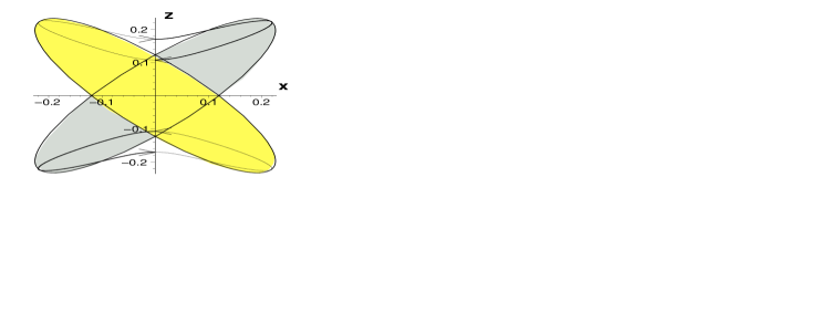
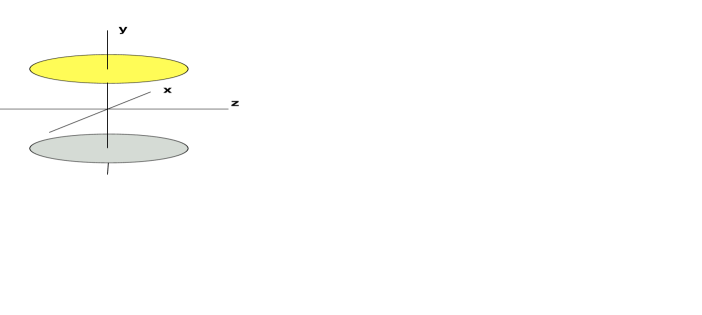
Figure 3: Location of the disk singularities (shading according to magnetic charge) for a so-called “rectangular” (left) and “crossed” (right) configuration, as used for the $Q=2$ solutions shown in resp. Fig. 2 and Fig. 4. Curves for the “crossed” give a one parameter family of solutions interpolating between two axially symmetric solutions for which ${\bf k}=1$ independent of ${\cal{D}}$ (see Ref. [12]).

Monopoles of different charges have to adjust to each other to form an exact caloron solution, such that ${\bf k}$ and ${\cal{D}}$ are in general not independent. So far we constructed two classes of solutions illustrated in Fig. 3 for both of which a large value of ${\cal{D}}$ implies that ${\bf k}$ approaches 1 exponentially. Hence we find point-like constituents, a necessary requirement to describe the field configurations at larger distances in terms of these objects. When all constituents of other types are sent to infinity, we recover the exact multi-monopole solutions of a given type of magnetic charge, and our results therefore also provide explicit solutions for the monopole zero modes, which were not known before for the multi-monopole configurations.

Surprisingly, the charge distribution giving rise to the abelian field far from any of the constituent cores (even when extended due to overlap) can be calculated exactly from ${\cal{V}}_{m}(\vec{x})$. For SU(2) we can parametrize the holonomy by ${{\cal P}_{\infty}}=\exp(2\pi i\vec{\omega}\cdot\vec{\tau})$ ($\mu_{2}\!=\!-\mu_{1}\!=\!|\vec{\omega}|$), where $\tau_{a}$ are the usual Pauli matrices. The field asymptotically becomes abelian, and is necessarily proportional to $\hat{\omega}\cdot\vec{\tau}$. Hence $A^{\rm{ff}}_{0}(\vec{x})=2\pi i\vec{\omega}\cdot\vec{\tau}-{\scriptstyle{\frac{1}{2}}}i\hat{\omega}\cdot\vec{\tau}\Phi(\vec{x})$, where the constant term shows again how $A_{0}$ plays the role of a Higgs field. For $Q=1$ and $2$ we have shown that $\Phi(\vec{x})=2\pi({\cal{V}}_{1}(\vec{x})-{\cal{V}}_{2}(\vec{x}))$. Therefore, the singularity structure in the zero-mode density agrees exactly with the abelian charge distribution, as given by $\partial_{i}^{2}\Phi(\vec{x})$. Outside the cores there is no source for the abelian field, implying $A_{0}$ to be harmonic in the far field (as is also clear from the relation to ${\cal{V}}_{m}$), and we find for the action density

$${\cal{S}}^{\rm{ff}}(\vec{x})=-2{\rm Tr}(\partial_{i}A_{0}(\vec{x}))^{2}=-\partial_{i}^{2}\Phi^{2}(\vec{x}).$$ (11)

Our expectation is that the result for $A_{0}^{\rm{ff}}(\vec{x})$ will hold for arbitrary $Q$ and will generalize to SU($n$) with each ${\cal{V}}_{m}(\vec{x})$ simply associated to the U(1) generator with respect to which the magnetic charge of the monopole of type $m$ is defined.

2.2 The construction – in brief

A charge $Q$ caloron with non-trivial holonomy is found with the Atiyah-Drinfeld-Hitchin-Manin formalism [17] by placing $|Q|$ instantons in the time interval $[0,b]$, which are repeated for each shift of $t$ over $b$, after a color rotation with ${{\cal P}_{\infty}}$. The resulting infinite topological charge is dealt with by Fourier transformation, relating it to the Nahm transformation for calorons [2]. The variable $z$ we introduced in formulating the generalized boundary conditions for the chiral fermions is precisely the dual of $t$ under this transformation. Singularities are introduced at $z=\mu_{m}$ through the powers of ${{\cal P}_{\infty}}$, as is seen from writing ${{\cal P}_{\infty}}=\sum_{m}e^{2\pi i\mu_{m}}P_{m}$ in terms of the $n$ projectors $P_{m}$. The Fourier transformation also produces $\hat{A}(z)$ as a U($|Q|$) gauge field on a circle, which satisfies the Nahm equation

$$\!\!\!\!\!{\frac{d}{dz}}\hat{A}_{j}(z)+[\hat{A}_{0}(z),\hat{A}_{j}(z)]+{\scriptstyle{\frac{1}{2}}}\varepsilon_{jk\ell}[\hat{A}_{k}(z),\hat{A}_{\ell}(z)]$$

$$\hskip 56.9055pt=2\pi i\sum_{m}\delta(z-\mu_{m})\rho_{m}^{\,j},$$ (12)

where $2\pi\zeta_{a}^{\dagger}P_{m}\zeta_{b}\!\equiv\!\Eins_{2}\hat{S}_{m}^{ab}\!-\!\vec{\tau}\cdot\vec{\rho}_{m}^{\,ab}$, with $\zeta_{b}$ two-component spinors in the $\bar{n}$ representation of SU($n$). Between the singularities $\hat{A}(z)$ is constant when $Q\!=\!1$, and for $Q\!=\!2$ it can be given [18] in terms of the Jacobi elliptic functions ${\rm sn}_{\bf k}$, ${\rm cn}_{\bf k}$ and ${\rm dn}_{\bf k}$.

The Green’s function $\hat{f}_{x}(z,z^{\prime})$ (cmp. Eq. (7)) is given by $\hat{g}^{\dagger}(z)f_{x}(z,z^{\prime})\hat{g}(z^{\prime})$, defined through

$$\left\{-\frac{d^{2}}{dz^{2}}+V(z;\vec{x})\right\}\!f_{x}(z,z^{\prime})=4\pi^{2}\delta(z\!-\!z^{\prime})\Eins,$$ (13)

with $V(z;\vec{x})\equiv 4\pi^{2}\vec{R}^{2}(z;\vec{x})+2\pi\sum_{m}\delta(z-\mu_{m})S_{m}$, $R_{j}(z;\vec{x})\equiv x_{j}-(2\pi i)^{-1}\hat{g}(z)\hat{A}_{j}(z)\hat{g}^{\dagger}(z)$ and $S_{m}\equiv\hat{g}(\mu_{m})\hat{S}_{m}\hat{g}^{\dagger}(\mu_{m})$. Note the latter play the role of “impurities”. The “dual” gauge function $\hat{g}(z)\equiv\exp(2\pi i(\xi_{0}-x_{0}\Eins)z)$, defined in terms of the dual holonomy $\exp(2\pi i\xi_{0})\equiv{\rm Pexp}(\int_{0}^{1}\hat{A}_{0}(z)dz)$, can be used to transform $\hat{A}_{0}-2\pi ix_{0}\Eins$ to zero, in order to simplify as much as possible the Green’s function equation. Although $\hat{f}_{x}(z,z^{\prime})$ is periodic in $z$ and $z^{\prime}$ with period $b$, $f_{x}(z,z^{\prime})$ no longer is.

Given a solution for the Green’s function, there are straightforward expressions for the gauge field [19] only involving the Green’s function evaluated at the “impurity” locations and for the fermion zero modes [12]. For the zero-mode density see Eq. (7). As an example we give the Green’s function at $z^{\prime}=z$, which formally can be expressed as (the $x$ dependence of ${\cal{F}}_{z}$ is implicit) $f_{x}(z,z)\!=\!-4\pi^{2}\left((\Eins\!-\!{\cal{F}}_{z})^{-1}\right)_{12}$, where the $(1,2)$ component on the right-hand side of the first identity is with respect to the $2\!\times\!2$ block matrix structure, each of size $|Q|\!\times\!|Q|$, and

$${\cal{F}}_{z}\!\equiv\!\hat{g}^{\dagger}(1){\rm Pexp}\!\int_{z}^{z+1}\!\!dw\pmatrix{0&\Eins\cr V(w;\vec{x})&0\cr}.$$ (14)

This has allowed us to find a compact formula for the action density [19],

$${\rm Tr}F_{\mu\nu}^{2}(x)\!=\!\partial_{\mu}^{2}\partial_{\nu}^{2}\log\det\left(ie^{-\pi ix_{0}}(\Eins\!-\!{\cal{F}}_{z})\right)\!,$$ (15)

which is actually independent of $z$ and reduces for Q=1 to Eq. (6).

The formal expression for ${\cal{F}}_{z}$ can be simplified with ${\cal{F}}_{z}\!=\!W_{m}(z)W_{m}^{-1}(\mu_{m}){\cal{F}}_{\mu_{m}}W_{m}(\mu_{m})W_{m}^{-1}(z)$, and decomposing ${\cal{F}}_{\mu_{m}}$ into “impurity” contributions at $z\!=\!\mu_{m}$ and the “propagation” between them, resp. $T_{m}$ and $H_{m}\!\equiv\!W_{m}(\mu_{m+1})W^{-1}(\mu_{m})$, with $T_{m}$, $W_{m}(z)$ and ${\cal{F}}_{\mu_{m}}$ given by

$$\hskip-11.38109ptT_{m}\!\!\equiv\!\!\pmatrix{\!\Eins&\!\!\!\!0\cr\!2\pi S_{m}&\!\!\!\!\Eins\cr}\!,\,W_{m}(z)\!\equiv\!\!\pmatrix{\ f_{m}^{+}(z)&f_{m}^{-}(z)\!\cr\!{\frac{d}{dz}}f^{+}_{m}(z)\!&\!\!{\frac{d}{dz}}f^{-}_{m}(z)\!\!\cr}\!,\!\!\!\!\!\!$$

$$\hskip-42.67912pt{\cal{F}}_{\mu_{m}}\!\equiv\!T_{m}\cdots H_{1}T_{1}\hat{g}^{\dagger}(1)H_{n}\cdots T_{m+1}H_{m},\!\!$$ (16)

The matrices $f_{m}^{\pm}(z)$, defined for $z\!\in\!(\mu_{m},\mu_{m+1})$, satisfy $f_{m}^{\pm}(z)\to\exp\left(\pm 2\pi|\vec{x}|(z-\mu_{m})\right)f_{m}(\mu_{m})$ for $|\vec{x}|\to\infty$. Together these form the $2|Q|$ solutions of the homogeneous Green’s function equation. To resolve the full structure of the cores for $Q=2$ we had to find the exact solutions for $f_{m}^{\pm}(z)$ on each interval. For this task we could make convenient use of an existing analytic result for charge 2 monopoles [20], adapting it to the case of calorons. Essential is that once $f_{m}^{\pm}(z)$ are known, everything else can be easily determined in terms of these, cmp. Eq. (16). A sample of the results [12] can be found in

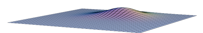
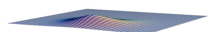
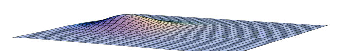
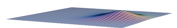
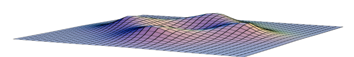
Figure 4: In the middle is shown the action density in the plane of the constituents at $t=0$ for an SU(2) charge 2 caloron with ${\rm Tr}\,{{\cal P}_{\infty}}=0$ in the “crossed” configuration of Fig. 3. On a scale enhanced by a factor $10\pi^{2}$ are shown the densities for the two zero modes, using either periodic (left) or anti-periodic (right) boundary conditions in the time direction.

Fig. 2 and Fig. 4.

3 Cooling studies for SU(2)

Dissociated calorons in a dynamical setting were first observed for SU(2), using cooling to analyze Monte Carlo generated lattice configurations just below $T_{c}$ [10]. Yet, applying the same methods for a symmetric box, corresponding to low temperatures, no dissociation was seen [15], in contrast to what was suggested by a fermionic zero-mode study [21]. Motivated by this we recently performed lattice cooling studies for SU(2), both at finite and low temperatures, to analyze the constituent nature of self-dual configurations in more detail [22]. At finite temperature this can be compared with the analytic results, but such results are not available for the symmetric torus. We used so-called $\varepsilon$-cooling [23], i.e. cooling with the improved action ($\raisebox{-5.69046pt}{ \begin{picture}(1.2,1.2)(-0.6,-0.6)\put(0.5,0.0){\line(-1,0){1.0}} \put(0.0,0.0){\vector(1,0){0.1}} \put(-0.5,0.0){\circle*{0.2}} \put(-0.35,-0.25){\makebox(0.0,0.0)[tr]{\footnotesize$x$}} \put(0.4,-0.3){\makebox(0.0,0.0)[r]{\footnotesize$\mu$}} \end{picture}}\equiv U_{\mu}(x)\in{\rm SU}(n)$)

$$S(\varepsilon) = \sum_{x,\mu,\nu}\xi_{\mu}\xi_{\nu}\Biggl{\{}\frac{4-\varepsilon}{3}\,\mathrm{Re}~{}{\rm Tr}\left(\Eins-\raisebox{-5.69046pt}{ \begin{picture}(1.2,1.2)(-0.6,-0.6) \put(-0.5,-0.5){\line(1,0){1.0}} \put(0.5,-0.5){\line(0,1){1.0}} \put(0.5,0.5){\line(-1,0){1.0}} \put(-0.5,0.5){\line(0,-1){1.0}} \put(0.0,-0.5){\vector(1,0){0.0}} \put(0.5,0.0){\vector(0,1){0.0}} \put(0.0,0.5){\vector(-1,0){0.0}} \put(-0.5,0.0){\vector(0,-1){0.0}} \put(-0.5,-0.5){\circle*{0.2}} \put(-0.55,-0.55){\makebox(0.0,0.0)[tr]{\footnotesize$x$}} \put(-0.55,0.0){\makebox(0.0,0.0)[r]{\footnotesize$\nu$}} \put(0.0,-0.55){\makebox(0.0,0.0)[t]{\footnotesize$\mu$}} \end{picture}}\right)$$ (17)

$$+ \frac{\varepsilon-1}{48}\,\mathrm{Re}~{}{\rm Tr}\Biggl{(}\Eins-\raisebox{-14.22636pt}{ \begin{picture}(1.2,1.2)(-0.6,-0.6) \put(-0.5,-0.5){\line(1,0){1.0}} \put(0.5,-0.5){\line(0,1){1.0}} \put(0.5,0.5){\line(-1,0){1.0}} \put(-0.5,0.5){\line(0,-1){1.0}} \put(-0.5,-0.5){\circle*{0.1}} \put(-0.5,0.5){\circle*{0.1}} \put(0.5,-0.5){\circle*{0.1}} \put(0.5,0.5){\circle*{0.1}} \put(0.0,-0.5){\circle*{0.1}} \put(0.0,0.5){\circle*{0.1}} \put(0.5,0.0){\circle*{0.1}} \put(-0.5,0.0){\circle*{0.1}} \put(-0.25,-0.5){\vector(1,0){0.0}} \put(0.25,-0.5){\vector(1,0){0.0}} \put(0.5,-0.25){\vector(0,1){0.0}} \put(0.5,0.25){\vector(0,1){0.0}} \put(-0.25,0.5){\vector(-1,0){0.0}} \put(0.25,0.5){\vector(-1,0){0.0}} \put(-0.5,-0.25){\vector(0,-1){0.0}} \put(-0.5,0.25){\vector(0,-1){0.0}} \put(-0.55,-0.55){\makebox(0.0,0.0)[tr]{\footnotesize$x$}} \put(-0.55,0.0){\makebox(0.0,0.0)[r]{\footnotesize$\nu$}} \put(0.0,-0.55){\makebox(0.0,0.0)[t]{\footnotesize$\mu$}} \end{picture}}\Biggr{)}\Biggr{\}}\;.$$

The ${\cal{O}}(a^{2})$ lattice artifacts are proportional to $\varepsilon$, and cause instantons to shrink for the Wilson action, which is recovered by putting $\varepsilon=1$. This shrinking can be stabilized with $\varepsilon=0$ or reversed with $\varepsilon<0$, which was therefore called over-improvement [23]. The $\xi_{\mu}$ are introduced to implement finite temperature (with $\xi_{0}=\xi^{\scriptstyle{3/2}}$ and $\xi_{i}=\xi^{-{\scriptstyle{1/2}}}$) on a symmetric lattice, using an anisotropic coupling $\xi$. In this way the temperature can be lowered in arbitrarily small steps, after each of which we perform some cooling adjusting the configuration to a solution at this temperature. We called this process “adiabatic” cooling. It allows us to start from a finite temperature configuration with well localized constituents, investigating how these evolve when lowering the temperature.

3.1 From finite to “zero” temperature

Constituents called instanton quarks were conjectured to play a role long ago [24]. Based on our experience with calorons, it is expected that when lowering the temperature the constituents will grow in size. In a finite volume, as used on the lattice, the maximal constituent separation is limited. We conclude that when $b=L$, i.e. for the symmetric box (which will be denoted by “zero” temperature), constituents necessarily overlap. In case of maximally non-trivial holonomy where all types of constituents are of equal mass, a periodic array of constituents is actually related to twisted instantons of fractional topological charge [25, 26]. As soon as the constituents are not equidistant, they tend to merge and can no longer be identified from their action density profiles. In Fig. 5 we present an example starting with two well-separated constituents at finite temperature (using $\xi=4$ on a $16^{4}$ lattice), lowering the temperature by reducing $\xi$ to 1.

Figure 5: Starting from a continuum caloron solution with well-separated lumps, discretized on the anisotropic lattice and adjusted to the finite volume by 100 $\varepsilon=-10$ cooling sweeps, we reduced $\xi$ from 4 to 1, through $\xi=2\sqrt{2}$, 2 and $\sqrt{2}$, applying between each of the 4 steps 100 $\varepsilon=-10$ cooling sweeps. Shown is the action density (top) and the the Polyakov loop in the time direction (bottom) along a line through the constituent locations. The dotted, dashed and full curves are for $\xi=4$, 2 and 1.

There is one minor complication, that on a torus no charge one self-dual solutions with finite size can exist, as can be proven with the help of the Nahm transformation [27]. This means that charge 1 instantons shrink (equivalent to the constituents getting closer) even when cooling with an action that has no lattice artifacts. This is why over-improvement was used in Fig. 5 to counteract this obstruction. In Figs. 7 and 7 the result for the adiabatic cooling of a charge 2 caloron which is free from such obstructions is shown. For Fig. 7 we start at finite temperature with the so-called “crossed” configuration (see Fig. 3, right).

In Fig. 7 the starting point at finite temperature (top) is the “rectangular” configuration (see Fig. 3, left). It has ${\rm Tr}\,{{\cal P}_{\infty}}=0$ and was taken from a Monte Carlo generated configuration at $\beta=2.2$, first cooling down to slightly above the 2 instanton action with $\varepsilon=1$. After this, many thousands of $\varepsilon=-2$ cooling sweeps were performed, followed by 500 with $\varepsilon=0$. We only show the action density in the plane through one of the two doughnut structures, the other doughnut is separated by half a period along the axis of symmetry. (The periodic zero modes are localized to one doughnut, and the anti-periodic zero modes to the other [12, 22]). To reach this configuration, we made use of the fact that under over-improved cooling constituents with opposite magnetic charge “repel” whereas those with the same magnetic charge “attract”, giving rise to constituents of equal magnetic charge to be exactly on top of each other.

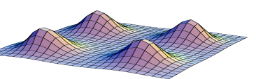
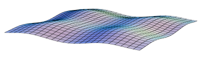
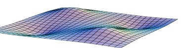
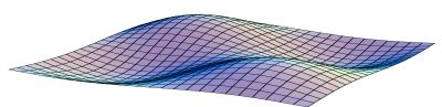
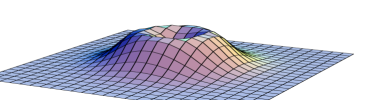
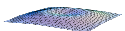
Figure 6: Starting at finite temperature with a charge 2 caloron in the “crossed” configuration on a $16^{4}$ lattice with $\xi=4$ after 1000 cooling sweeps with $\varepsilon=0$ (left two figures), changing $\xi$ through $2\sqrt{2}$, 2, $\sqrt{2}$ to reach 1 (right two figures), at each of these applying 1000 cooling sweeps with $\varepsilon=0$. The top plots show the action density integrated over time, the bottom plots the Polyakov loop in the time direction, both in the $y$-$z$ plane at $x=8$ (where all constituents lie).

Figure 7: As in Fig. 7 but now starting from a “rectangular” configuration first made at finite temperature ($\xi=4$, left) as described in the text. The action densities ($\xi=1$, right) integrated over time, is shown in the plane of the doughnut.

The adiabatic cooling is performed with $\varepsilon=0$ cooling to prevent such “forces” due to the lattice artifacts while lowering the temperature. But when applying cooling with $\varepsilon=-10$, the “fat” doughnut (see Fig. 7, right) ultimately will reach the self-dual constant curvature solution that is allowed [28, 29] for a symmetric box with $Q=2$.

There is another way to avoid the $Q=1$ obstruction on a torus, namely by using twisted boundary conditions [25], as was used for the study of calorons before [13]. Under much prolonged over-improved cooling with a twist in the $0$-$i$ planes we found somewhat to our surprise that it was possible to push the constituents further apart than half a period, at the same time inverting the magnetic charge of one constituent with respect to the other (this is in part due to the fact that the Polyakov loop is anti-periodic in the $i$-th direction due to the twist, for more details see Ref. [22]). This ultimately gave a perfect doughnut, i.e. two magnetic monopoles of equal charge on top of each other.

All these studies [22] have shown that at low temperatures constituents are not localized to better than half the size of the volume, both for the action density and chiral zero modes. We conclude that well-localized lumps at zero temperature for low-charge self-dual backgrounds can only be found as instantons, even though it is clear that these are built from constituents of fractional topological charge, as seen through the behavior of the Polyakov loop. A good measure for the zero-mode localization [11] is the inverse participation ratio, $I\equiv V\sum_{x}\rho^{2}(x)$, where $\rho(x)$ is the zero-mode density $\hat{\Psi}_{z}^{\dagger}(x)\hat{\Psi}_{z}(x)$. The bigger $I$ is, the more localized is the zero mode. This can be contrasted with a constant zero-mode density for which $I=1$. On average, at finite temperature [11] $I$ is indeed considerably larger than at zero temperature [21], but in the latter case values of $I$ as big as 20 or more are still seen to occur for cases where zero modes jump over distances as large as half the size of the volume when cycling through the boundary conditions. For our low-charge self-dual backgrounds the zero modes associated with separated constituents never reached values of $I$ above 2.

The possibility that the zero modes are localized to instantons (formed from closely bound constituents) and jump between well-separated instantons, rather than well-separated isolated constituents, was discussed in Ref. [30]. It was found that at finite temperature this is unlikely to occur, but it could not be ruled out for zero temperature. In a random medium of topological lumps the mechanism of localization of the zero modes could very well be similar to Anderson localization. In such a case one perhaps should expect a dependence on the fermion boundary conditions, even when constituents remain well hidden inside instantons. In the case that instantons form a dense ensemble, this is similar to the statement that it is impossible to determine which set of constituents forms an instanton. That some of the zero modes, if associated to fractionally charged lumps, are more localized than we observed [22] can have a dynamical origin.

3.2 Cooling histories

That for temperatures just below $T_{c}$ well dissociated calorons are seen from the action density profiles has now been well established [10]. Nevertheless, it is interesting that this can be deduced also from inspecting the cooling histories obtained with the Wilson action.

$({\bf s})$

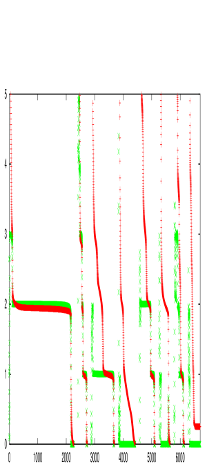
Figure 8: Sample of 8 histories on a $16^{3}\times 4$ lattice at $\beta=2.2$ ($T\approx 0.8T_{c}$). Pluses give the Wilson action and crosses the absolute value of the (order $a^{2}$ improved clover averaged) topological charge.

There are three processes under which the action is lowered during cooling. The first and most important one is the removal of short distance fluctuations. Next is the annihilation of lumps with opposite topological charge, and last the falling of instantons through the lattice due to its shrinking. Annihilation can, however, also occur between well-localized lumps of opposite fractional topological charge.

To detect these events one defines a plateau in the cooling history as the point of inflection for the action as a function of the cooling sweeps (i.e. when the decrease per step becomes minimal) [10]. In the confined phase, where on average the charge fraction is one half, the change in action would typically be around one unit, and the topological charge would remain unchanged (an example is indicated by “s” in Fig. 8). This can thus be easily distinguished from the annihilation of an instanton and anti-instanton, for which the action changes by two units. On the other

(i)                 (ii)                 (iii)

Figure 9: Scatterplots of $|\Delta Q|$ (horizontally) versus $\Delta S$ (vertically) for a $6^{3}\times 4$ lattice at (i) $\beta=2.4$ ($T\approx 1.2T_{c}$), (ii) $\beta=2.2$ ($T\approx 0.8T_{c}$), and (iii) a $16^{4}$ lattice at $\beta=2.3$ ($T\approx 0.25T_{c}$).

hand, when an instanton falls through the lattice (i.e. two constituents with the same sign for their fractional topological charge, but of opposite magnetic and electric charge, come together and form a localized instanton, which then shrinks under cooling) both the topological charge and the action changes by one unit.

We collected the information concerning cooling histories in scatterplots, each based on 50 Monte Carlo generated configuration, see Fig. 9. Only for $T$ just below $T_{c}$ the constituents are sufficiently well localized to give rise to clear constituent annihilations as seen from the clustering of $(\Delta S,|\Delta Q|)$ around $(1,0)$, measured from one plateau to the next.

The presence of constituents of opposite topological charge also gives rise to the interesting fact that the number of near zero modes (in a smooth, but non-selfdual background) can depend on the fermion boundary conditions as shown in Fig. 10. The anti-periodic zero modes localize to constituents for which the Polyakov loop is $-1$, whereas for periodic zero modes $P=+1$. The underlying configuration of Fig. 10 has 3 anti-selfdual lumps of which one has $P=+1$ and one self-dual lump with $P=-1$. Thus there are three anti-periodic near zero modes, two of which disappear as soon as $z\neq{\scriptstyle{\frac{1}{2}}}$.

Im$\,\lambda$
                                   Re$\,\lambda$

Figure 10: Zero-modes for an anti-caloron on a $16^{3}\!\times\!4$ lattice, with in addition two constituents of opposite fractional topological charge. Crosses give the low-lying eigenvalues $\lambda$ of the clover-improved Wilson-Dirac operator with periodic boundary conditions in time. The curves trace two near zero modes from their value with anti-periodic (left) boundary conditions to the periodic (right) case, in 5 equal steps in $z$ (squares).

4 Marginally stable configurations

The last cooling run shown in Fig. 8 ends in a configuration with $Q=0$ and $S\approx 1/4$ units, which is stable under further cooling. These so-called Dirac sheets had been shown to typically arise after constituent annihilation, leaving a constant magnetic field [31]. It is perhaps surprising that such constant magnetic fields can be stable, but this is a consequence of the finite volume in which a non-trivial holonomy can affect the fluctuation spectrum. Since the action of the constant magnetic field does not depend on the holonomy, which also holds on the lattice, this was called marginal stability [32] and explains the stability under further cooling, once it is reached.

The finite temperature setting is essential, as otherwise one would need to introduce twisted boundary conditions to construct marginally stable configurations [32]. For $SU(2)$ the constant magnetic field solutions are in fact abelian, with $F_{\mu\nu}=\pi i\tau_{3}n_{\mu\nu}/(L_{\mu}L_{\nu})$ in a suitable gauge. Here $n_{\mu\nu}$ is antisymmetric, taking even integer values (in the absence of twisted boundary conditions). Adding a constant to the abelian vector potential can be partly, but not completely, absorbed by a translation. The part that cannot be absorbed will affect the fluctuation spectrum. With $L_{i}\!=\!L$, $n_{0\nu}\!=\!0$ and $m_{i}\!=\!{\scriptstyle{\frac{1}{2}}}\varepsilon_{ijk}n_{jk}$, the eigenvalues for the quadratic fluctuations can be shown to be [29, 32] $\lambda_{\pm}\!\!=\!2\pi(2n+\!1\pm 2)|\vec{m}|/L^{2}\!+(2\pi ep+\!\vec{m}\cdot\vec{C})^{2}\!/(|\vec{m}|L)^{2}\!+(2\pi q\!+\!C_{0})^{2}/b^{2}$ and $\lambda_{0}=(2\pi k_{\mu}/L_{\mu})^{2}$, with multiplicities resp. $2|e|$ and 2, where $e$ is the greatest common divisor of the $m_{i}$. All quantum numbers ($n,p,q,k_{\mu}$) are integer (but $n\geq 0$).

At finite temperature the spatial holonomies are typically trivial and the relevant Polyakov loop to consider for the dependence on the spectrum is $P_{0}={\scriptstyle{\frac{1}{2}}}{\rm Tr}\exp(iC_{0}\tau_{3}/2)=\cos(C_{0}/2)$ or rather $P_{0}^{2}$. This is because the fluctuations involve adjoint fields and the spectrum is periodic under a shift of $C_{0}$ over $2\pi$, whereas $P_{0}$ is anti-periodic. To find the lowest eigenvalue we put $n\!=\!q\!=\!p_{i}\!=\!C_{i}\!=\!0$ (we may restrict $|C_{0}|\leq\pi$) such that $\lambda_{-}=-2\pi|\vec{m}|/L^{2}+C_{0}^{2}/b^{2}$ is negative unless the Polyakov loop $P_{0}$ is sufficiently non-trivial. All eigenvalues are therefore positive when

$$|\vec{m}|<\frac{L\sqrt{\pi}}{b}\quad\mbox{and}\quad|P_{0}|<\cos\left(\frac{|\vec{m}|b\sqrt{\pi}}{2L}\right).$$ (18)

These conditions can never be satisfied when $b=L$, nor in the deconfined phase where the Polyakov loop is too close to being trivial. We found in the cooling histories on $16^{3}\times 4$ lattices stable configurations with one, two and three quarters of the instanton action (with one, two or three of the components of $\vec{m}$ being 2). For the minimal case, $|\vec{m}|=2$, the correlation between stability and the value of the Polyakov loop was studied in much detail [33], showing perfect agreement with the analytic prediction in Eq. (18).

5 Lattice calorons for SU(3)

Caloron solutions with non-trivial holonomy for SU(3) are qualitatively different from those with trivial holonomy and from embedded SU(2) solutions, which appear only as limiting cases. We will illustrate this with generic SU(3) solutions obtained by cooling on a finite lattice.

First we consider a $Q\!=\!2$ solution on a $20^{3}\!\times\!4$ lattice, see Fig. 11.

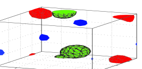
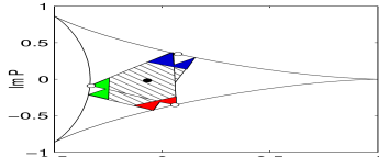
Figure 11: Shown on the left by colored spheres are the six constituent monopoles for a $Q=2$ caloron. The behavior of the Polyakov loop is shown on the right, with the filled circle corresponding to the holonomy and the three open circles to the predicted values of $P$ at the constituent locations. The actual values of $P$ for points in their neighborhood are represented by the colored corners.

Eigenvalues of the Polyakov loop all agree very well in the region where the action density is lowest (10 % of the volume), and are used to define the holonomy ${{\cal P}_{\infty}}$ in the case of a finite lattice. For calorons with one unit of topological charge it can be shown [14] that at the positions where two eigenvalues of the Polyakov loop coincide, these eigenvalues are given resp. by $\{e^{-\pi i\mu_{3}},e^{-\pi i\mu_{3}},e^{2\pi i\mu_{3}}\}$, $\{e^{2\pi i\mu_{1}},e^{-\pi i\mu_{1}},e^{-\pi i\mu_{1}}\}$, and $\{-e^{-\pi i\mu_{2}},e^{2\pi i\mu_{2}},-e^{-\pi i\mu_{2}}\}$. This is tested on the right in Fig. 11. The typical range for $P$ (one-third the trace of the Polyakov loop) is shown for two hypothetical $Q\!=\!1$ objects. It is spanned by the colored corners which correspond to the actual values inside the cores of the constituent monopoles. The colors distinguish the three different types of monopoles. For clarity we do not show the full scatterplot for $P$. The boundary for the range of $P$ values in the complex plane is indicated by the curved triangle. The closeness of two of the three eigenvalues is represented by the distance to this boundary. The six isosurfaces of that distance function are pictured in corresponding colors on the left in Fig. 11, this is also where the action or topological charge density (not shown) is maximal.

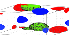
Figure 12: The positions (red, blue, green) of the two zero modes (left) for the charge 2 configuration shown in Fig. 11 with the $z$ values corresponding to the maxima of $I$ (shown on the right).

The two zero modes for the charge 2 configuration of Fig. 11 are shown on the left of Fig. 12 as isosurfaces of its zero-mode density. Using colors we combine in one figure three values of $z$ that specify the fermion boundary condition in the time direction. These $z$ values correspond to the three maxima of the inverse participation ratio [11] $I$ (shown on the right), for which the zero modes are maximally localized. The monopole locations defined through the coinciding eigenvalues of the Polyakov loop agree (within one lattice spacing) with the maxima of the zero-mode density. With help of the $z$-dependent zero modes one can focus on one of the three types of monopoles alone, which brings out more clearly the constituent nature of calorons.

Compared with the analytic caloron solutions with arbitrary holonomy for $S^{1}\times\mathbb{R}^{3}$, lattice solutions have imperfections, some specific for SU(3). These are caused by the finite volume with periodic boundary conditions (leading to the charge one obstruction discussed in Sect. 3) and its finite aspect ratio $b/L$, as well as by lattice artifacts. Hence, several compromises are necessary to describe the moduli space of caloron solutions using cooling on the lattice. In this spirit we have performed a systematic investigation [34] of the structure of SU(3) calorons with $|Q|=1,2,3$ and 4 on $N_{s}^{3}\times N_{t}$ lattices with $N_{s}=12$ and 20 ($N_{t}\geq 4$). For $N_{s}=12$ the results are based on ${\cal{O}}(10000)$ cooled configurations. The holonomy is non-trivial when applying cooling to configurations generated in the confined phase using $\beta=5.6$ (corresponding to $T\approx 0.95T_{c}$ for $N_{t}=4$). Similar to what was seen for SU(2) [10], the distribution of the Polyakov loop broadens with cooling, and cuts in $P_{\infty}\!=\!{\rm Tr}\,{{\cal P}_{\infty}}/3$ are sometimes helpful to highlight the constituent nature.

For an automated scanning of the solutions we introduced two observables, the non-staticity [10] $\delta_{t}\!\equiv\!\frac{N_{t}}{4}\sum_{x}\left|s(x)-\!s(x\!+\!\hat{t})\right|/S$ and the violation of (anti)self-duality $\delta_{F}\!\equiv\!\sum_{x}\left|s(x)\!-\!8\pi^{2}|q(x)|\right|/S$. The non-staticity is used to determine when separated lumps are seen within a solution. Points of bifurcation occur when $\delta_{t}^{*}=0.27$ and $\delta_{t}^{**}=0.06$ for which respectively two and three peaks become visible in the topological charge density. These values were estimated on the basis of the exact charge one caloron solutions with maximally non-trivial holonomy and suitably arranged constituents [34]. The ${\cal{O}}(a^{4})$-improved field strength [35] was used to construct the action and topological charge densities, to minimize the effect of lattice artifacts. For the fermions with adjustable boundary conditions we used the clover-improved Wilson-Dirac operator.

Like for SU(2), instantons and calorons shrink under cooling with the Wilson action. In addition, charge one caloron solutions can only be obtained at the expense of violation of (anti)self-duality. For example, cooling on a $16^{3}\!\times\!4$ lattice with a stopping criterion based on a minimal violation of the lattice equations of motion [10], or a minimal value of $\delta_{F}$, one is unable to produce dissociated $|Q|=1$ calorons, although this can be corrected for using over-improved cooling, as we have seen for SU(2) in Sect. 3. However, for our high-statistics study we have restricted ourselves to Wilson-type cooling. Instead we modified the condition under which cooling is stopped and the approximate solution is stored.

The extended stopping criterion is based on either the non-staticity $\delta_{t}$ or the violation of (anti)self-duality $\delta_{F}$ to pass through a minimum. The distribution of (almost) classical solutions on a $12^{3}\times 4$ lattice with respect to $\delta_{t}$ is compared for both cases in the upper row of Fig. 13.

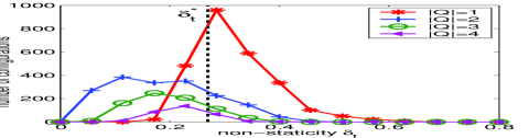
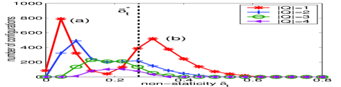
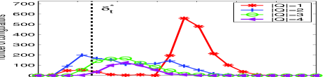
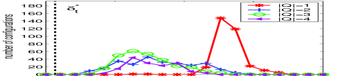
Figure 13: Histograms of non-staticity $\delta_{t}$ for configurations obtained when the violation of (anti)self-duality $\delta_{F}$ is minimal (upper left) and when using the extended stopping criterion described in the text (upper right), both on a $12^{3}\!\times\!4$ lattice. The bottom row shows the results for $12^{3}\!\times\!6$ (left) and $12^{4}$ (right) lattices, also using the extended stopping criterion.

The vertical line, drawn to guide the eye, represents $\delta_{t}^{*}$ where the bifurcation of 1 into 2 peaks occurs. With the modified stopping criterion, which allows for some violation of (anti)self-duality, many perfectly static calorons are found which are clearly split into constituents. These are marked by “(a)” on the top right plot in Fig. 13, to be contrasted with the behavior in the top left plot, and are mainly associated to $|Q|=1$ (with some $|Q|=2$) configurations. Yet all satisfy $\delta_{F}<0.2$, and are sufficiently close to a classical solution. In the lower row of Fig. 13 the distribution over $\delta_{t}$ is shown for approximate solutions found on lattices $12^{3}\times 6$ and $12^{4}$ (the symmetric torus), again using the extended stopping criterion. This confirms for SU(3) the tendency towards non-dissociated constituents also found for SU(2) [15] where it is now well understood [22], as was discussed in Sect. 3.

As emphasized before, constituent monopoles can be detected through the behavior of the Polyakov loop, even when they are close together. This is exemplified by Fig. 14 where the non-staticity

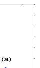
Figure 14: Correlation between the non-staticity $\delta_{t}$ and the average inter-monopole distance for charge one configurations on $12^{3}\times 4$.

is plotted versus the average inter-monopole distance for charge one calorons on $12^{3}\!\times\!4$ lattices. The two clusters marked “(a)” and “(b)” agree with the configurations associated to the two peaks marked in Fig. 13 for the top right plot, based on the extended stopping criterion.

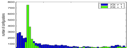
Figure 15: Histograms for the violation of (anti) self-duality $\delta_{F}$, separately for $|Q|=1$ and $|Q|>1$ on a lattice of size $12^{3}\times 4$.

It is interesting to see how $\delta_{F}$ is actually distributed. This is shown in Fig. 15 (where a cut in $\delta_{F}$ at 0.2 was applied) contrasting $|Q|=1$ with $|Q|>1$. Absence of configurations with charge one for $\delta_{F}\!<\!0.016$ illustrates the non-existence of self-dual fields with $|Q|=1$ on the torus.

Regardless of the number of lumps, our method of locating and counting monopoles described above is reliable provided the configurations have non-trivial holonomy. The number of monopoles is distributed very narrowly around $3|Q|$.

Figure 16: Average number of monopoles and of maxima of the topological density and their standard deviations as function of $|Q|$ for the $12^{3}\times 4$ lattice, without cuts (left), with a cut $|P_{\infty}|<0.2$ (center) and with an additional cut $\delta_{t}<0.2$ (right).

This is shown in Fig. 16 where the average number of monopoles and peaks in the topological charge density are represented as a function of $|Q|$, without cuts and with cuts in $|P_{\infty}|$ and $\delta_{t}$. These cuts effect the number of peaks but not the number of monopoles, which however does become more narrowly distributed.

We have thus seen that the approximate SU(3) caloron solutions produced by cooling, even on relatively small lattices, resemble the analytically known caloron solutions. The way they manifest themselves depends on the aspect ratio of the lattice.

6 Conclusions

We have seen that instantons at finite temperature are composed of constituent monopoles. More details for SU(3) will appear soon [34]. The hope is of course to be able to develop a calculational scheme to address questions like monopole condensation in the popular scenario of the dual superconductor [36]. From the analytic side this is complicated by the fact that at low temperature the coupling constant is large, and instantons form a dense ensemble. More detailed lattice studies would be welcome. A dense ensemble of instantons implies that the monopoles are dense as well. The confining electric phase could perhaps be characterized by a dual deconfining magnetic phase, where the dual deconfinement is due to the large monopole density, similar in spirit to high density induced quark deconfinement.

References

- [1] B.J. Harrington, H.K. Shepard, Phys. Rev. D17 (1978) 2122; Phys. Rev. D18 (1978) 2990.
- [2] W. Nahm, Self-dual monopoles and calorons, in: Lecture Notes in Physics 201 (1984) 189.
- [3] T.C. Kraan and P. van Baal, Phys. Lett. B428 (1998) 268; Nucl. Phys. B533 (1998) 627.
- [4] K. Lee, Phys. Lett B426 (1998) 323; K. Lee and C. Lu, Phys. Rev. D58 (1998) 025011.
- [5] T.C. Kraan and P. van Baal, Phys. Lett. B435 (1998) 389.
- [6] N. Weiss, Phys. Rev. D24 (1981) 475.
- [7] D. Diakonov, N. Gromov, V. Petrov and S. Slizovskiy, hep-th/0404042.
- [8] M.García Pérez, A.González-Arroyo, C.Pena and P. van Baal, Phys.Rev. D60(1999)031901.
- [9] M.N. Chernodub, T.C. Kraan, P. van Baal, Nucl. Phys. B(Proc.Suppl.)83-84 (2000) 556.
- [10] E.-M. Ilgenfritz et al., Phys. Rev. D66 (2002) 074503.
- [11] C. Gattringer and S. Schaefer, Nucl. Phys. B654 (2003) 30.
- [12] F. Bruckmann, D. Nógrádi and P. van Baal, Nucl.Phys. B666 (2003) 197; hep-th/0404210.
- [13] M. García Pérez et al., JHEP 06 (1999) 001.
- [14] P. van Baal, hep-th/9912035.
- [15] E.-M. Ilgenfritz et al., Phys. Rev. D69 (2004) 114505.
- [16] P. Forgács, Z. Horváth and L. Palla, Nucl. Phys. B192 (1981) 141.
- [17] M.F. Atiyah, N.J. Hitchin, V. Drinfeld and Yu.I. Manin, Phys. Lett. 65A (1978) 185.
- [18] W. Nahm, Multi-monopoles in the ADHM construction, in: Gauge theories and lepton hadron interactions, eds. Z. Horváth, ea. (Budapest, 1982); S.A. Brown, H. Panagopoulos and M.K. Prasad, Phys. Rev. D26 (1982) 854.
- [19] F. Bruckmann and P. van Baal, Nucl. Phys. B653 (2002) 105.
- [20] H. Panagopoulos, Phys. Rev. D28 (1983) 380.
- [21] C. Gattringer, R. Pullirsch, Phys.Rev. D69 (2004) 094510.
- [22] F. Bruckmann, E.-M. Ilgenfritz, B.M. Martemyanov and P. van Baal, hep-lat/0408004.
- [23] M. García Pérez et al., Nucl. Phys. B413 (1994) 535.
- [24] A.A. Belavin, V.A. Fateev, A.S. Schwarz and Y.S. Tyupkin, Phys. Lett. B83 (1979) 317.
- [25] G. ’t Hooft, Nucl. Phys. B153 (1979) 141; Acta Physica Aust. Suppl. XXII (1980) 531.
- [26] M. García Pérez, A. González-Arroyo and B. Söderberg, Phys. Lett. B235 (1990) 117.
- [27] P.J. Braam and P. van Baal, Comm. Math. Phys. 122 (1989) 267.
- [28] G. ’t Hooft, Comm. Math. Phys. 81 (1981) 267.
- [29] P. van Baal, Comm. Math. Phys. 94 (1984) 397.
- [30] F. Bruckmann et al., Nucl. Phys. B(Proc. Suppl.)129 (2004) 727.
- [31] E.-M. Ilgenfritz et al., Eur. Phys. J. C34 (2004) 439.
- [32] M. García Pérez and P. van Baal, Nucl. Phys. B429 (1994) 451.
- [33] E.-M. Ilgenfritz et al., Phys. Rev. D69 (2004) 097901.
- [34] D. Peschka, E.-M. Ilgenfritz and M. Müller-Preussker, in preparation.
- [35] S.O. Bilson-Thompson et al., Ann. Phys. 304 (2003) 1.
- [36] S. Mandelstam, Phys. Rept. 23 (1976) 245; G. ’t Hooft, in: High Energy Physics, ed. A. Zichichi (Bolognia, 1976); Nucl. Phys. B138 (1978) 1.