ROM2F/2004/20
DESY 04-144
FTUAM-04-19
IFT UAM-CSIC/04-45
August 2004
NLO anomalous dimension of multiplicatively renormalizable four–fermion operators in Schrödinger Functional schemes

Abstract

Renormalization constants for multiplicatively renormalizable parity-odd four–fermion operators are computed in various different Schrödinger Functional (SF) schemes and lattice regularizations with Wilson quarks at one–loop order in perturbation theory. Our results are used in the calculation of their NLO anomalous dimensions, through matching to continuum schemes. They also enable a comparison of the two–loop perturbative RG running to the previously obtained nonperturbative one in the region of small renormalized coupling.

1 Introduction

Four–fermion operators occur in the transition amplitudes of many physical processes within the SM and beyond. An example is provided by the oscillations of the $K^{0}-\bar{K}^{0}$ system, where the mixing amplitude is given by a matrix element of the form

$$\langle\bar{K}^{0}|{\cal O}^{+}_{\rm VV+AA}|K^{0}\rangle=\frac{8}{3}F_{K}^{2}m_{K}^{2}B_{K}.$$ (1)

Renormalizing the operator ${\cal O}^{+}_{\rm VV+AA}$ on the lattice with Wilson quarks requires special care, as it mixes with other four–fermion operators. The situation is simpler in the framework of tmQCD, where the operator in question can be mapped onto its parity-odd counterpart ${\cal O}^{+}_{\rm VA+AV}$, which is multiplicatively renormalizable [3]. Nonperturbative renormalization of the latter in SF schemes has been reported in [2], where its scale dependence has been computed in the continuum limit through finite size scaling techniques. On the other hand, the corresponding one–loop perturbative calculation is required in order to make contact to continuum schemes. It can also be used for an analytical estimation of the perturbative lattice artefacts.

2 SF renormalization

Renormalization of a local fermion operator is pursued in a SF scheme by imposing a suitable renormalization condition at vanishing renormalized quark mass on a correlation function, properly defined to probe the operator by bilinear boundary quark sources

$$S_{f_{1}f_{2}}[\Gamma] = a^{6}\sum_{\bf y,z}\ \bar{\zeta}_{f_{1}}({\bf y})\ \Gamma\ \zeta_{f_{2}}({\bf z}),$$ (2)

$$S^{\prime}_{f_{1}f_{2}}[\Gamma] = a^{6}\sum_{\bf y^{\prime},z^{\prime}}\ \bar{\zeta}_{f_{1}}^{\prime}({\bf y^{\prime}})\ \Gamma\ \zeta_{f_{2}}^{\prime}({\bf z^{\prime}}).$$ (4)

Here the boundary fields $\zeta$ and $\bar{\zeta}$ are defined at $x_{0}=0$, while $\zeta^{\prime}$ and $\bar{\zeta}^{\prime}$ are defined at $x_{0}=T$; $\Gamma$ is a generic Dirac matrix and $f_{i}$ are flavour indices. The simplest way to probe the four–fermion operator

$${\cal O}_{\rm VA+AV}^{\pm} = \frac{1}{2}\bigl{[}\bar{\psi}_{1}\gamma_{\mu}\psi_{2}\bar{\psi}_{3}\gamma_{\mu}\gamma_{5}\psi_{4}+$$ (6)

$$\ \ \ \bar{\psi}_{1}\gamma_{\mu}\gamma_{5}\psi_{2}\bar{\psi}_{3}\gamma_{\mu}\psi_{4}\pm(2\leftrightarrow 4)\bigr{]}$$

is by inserting it in a correlation function with three bilinear boundary sources

$$h^{\pm}(x_{0})=\frac{1}{L^{3}}\langle S^{\prime}_{53}[\Gamma_{3}]{\cal O}^{\pm}(x)S_{21}[\Gamma_{1}]S_{45}[\Gamma_{2}]\rangle.$$ (7)

Parity conservation implies that one has to provide a parity–odd choice of the set $[\Gamma_{1},\Gamma_{2},\Gamma_{3}]$ in order to get a nonvanishing correlation function. Provided this, the ultraviolet divergences of the boundary fields must be removed in order to isolate the divergences of the operator. To this purpose $h^{\pm}(x_{0})$ can be normalized as

$$\tilde{h}^{\pm}(x_{0})=\frac{h^{\pm}(x_{0})}{f_{1}^{\alpha}\ k_{1}^{\beta}}\biggr{|}_{\alpha+\beta=3/2},$$ (8)

where we have introduced the standard boundary correlation functions with no operator insertion

$$f_{1} = -\frac{1}{\ \ L^{6}}\langle S^{\prime}[\gamma_{5}]S[\gamma_{5}]\rangle,$$ (9)

$$k_{1} = -\frac{1}{3L^{6}}\sum_{k=1}^{3}\langle S^{\prime}[\gamma_{k}]S[\gamma_{k}]\rangle.$$ (10)

The condition $\alpha+\beta=3/2$ makes $\tilde{h}^{\pm}(x_{0})$ free of boundary divergences and suitable to be renormalized through a multiplicative condition

$$\tilde{h}_{R}^{\pm}(T/2)=\tilde{h}^{\pm}_{\rm tree}(T/2)\ \ {\rm at}\ m_{R}=0,$$ (11)

where the subtraction point is at $\mu=1/L$, $m_{R}$ is the renormalized quark mass, the operator ${\cal O}^{\pm}_{\rm VA+AV}$ is placed in the middle of the time extent of the SF and

$$\tilde{h}_{R}^{\pm}(T/2)=Z^{\pm}_{\rm VA+AV}(g_{0},a/L)\ \tilde{h}^{\pm}(T/2).$$ (12)

Apart from the indicated dependence, the renormalization constant $Z_{\rm VA+AV}^{\pm}$ depends upon every detail, such as the value of  $T/L$ (in this work $T/L=1$), the choice of the Dirac structure of the sources and the exponents $\alpha,\beta$ in eq. (5). A number of possible combinations exist, each one generating a different renormalization scheme in the framework of the SF. In Table 1 we report the ones we have considered.

scheme	$[\Gamma_{1},\Gamma_{2},\Gamma_{3}]$	$\alpha$	$\beta$
I	$[\gamma_{5},\gamma_{5},\gamma_{5}]$	$3/2$	$0$
II	$\frac{1}{6}\sum_{ijk=1}^{3}\epsilon_{ijk}[\gamma_{i},\gamma_{j},\gamma_{k}]$	$3/2$	$0$
III	$\frac{1}{3}\sum_{k=1}^{3}[\gamma_{5},\gamma_{k},\gamma_{k}]$	$3/2$	$0$
IV	$\frac{1}{3}\sum_{k=1}^{3}[\gamma_{k},\gamma_{5},\gamma_{k}]$	$3/2$	$0$
V	$\frac{1}{3}\sum_{k=1}^{3}[\gamma_{k},\gamma_{k},\gamma_{5}]$	$3/2$	$0$
VI	$\frac{1}{6}\sum_{ijk=1}^{3}\epsilon_{ijk}[\gamma_{i},\gamma_{j},\gamma_{k}]$	$0$	$3/2$
VII	$\frac{1}{3}\sum_{k=1}^{3}[\gamma_{5},\gamma_{k},\gamma_{k}]$	$1/2$	$1$
VIII	$\frac{1}{3}\sum_{k=1}^{3}[\gamma_{k},\gamma_{5},\gamma_{k}]$	$1/2$	$1$
IX	$\frac{1}{3}\sum_{k=1}^{3}[\gamma_{k},\gamma_{k},\gamma_{5}]$	$1/2$	$1$

Table 1:

3 One–loop perturbative expansion

In order to extract the one–loop contribution to the renormalization constant, all the correlation functions must be expanded in powers of the bare coupling,

$${\cal X}={\cal X}^{(0)}+g_{0}^{2}\biggl{[}{\cal X}^{(1)}+m_{c}^{(1)}\frac{\partial{\cal X}^{(0)}}{\partial m_{0}}\biggr{]}+O(g_{0}^{4}),$$ (13)

with ${\cal X}$ being $h^{\pm}$, $f_{1}$, $k_{1}$, as well as the renormalization constant itself,

$$Z^{\pm}_{\rm VA+AV}=1+g_{0}^{2}Z^{\pm(1)}_{\rm VA+AV}+O(g_{0}^{4}).$$ (14)

Terms proportional to the one–loop coefficient of the critical mass $m_{c}^{(1)}$ are needed to set the correlation functions to zero renormalized quark mass. The values of $f_{1}^{(0,1)}$ and $k_{1}^{(0,1)}$ are known from the literature [4], while $h^{\pm(0,1)}$ have been computed through numerical integration of the related Feynman diagrams for both Wilson and Clover actions. The analytic structure of $Z_{\rm VA+AV}^{\pm(1)}$ is provided by the “log”–divergent relation

$$Z_{\rm VA+AV}^{\pm(1)}=B^{\pm}_{\rm SF}+\gamma^{\pm(0)}\ln\left(\frac{a}{L}\right)+O\left(\frac{a}{L}\right),$$ (15)

where $\gamma^{\pm(0)}=\pm 6(1\mp 1/N)/(4\pi)^{2}$ is the LO anomalous dimension of ${\cal O}_{\rm VA+AV}^{\pm}$ and $B^{\pm}_{\rm SF}$ is a finite term, which depends upon the renormalization scheme and can be computed by inserting the perturbative expansion of the correlation functions and the renormalization constant in eq. (7).

4 Matching to DRED

Given the NLO (scheme dependent) anomalous dimension in a reference scheme, it can be computed in any other scheme, provided the one–loop order renormalization constant is known in the latter. In our case we choose DRED as the reference scheme, and the matching formula is given by

$$\gamma_{\rm SF}^{\pm(1)}=\gamma_{\rm DRED}^{\pm(1)}+2b_{0}\biggl{[}B^{\pm}_{\rm SF}-{z^{\pm}}\biggr{]}+\gamma^{\pm(0)}{c_{g}},$$ (16)

where the second term on the RHS measures the shift of the finite term of the one–loop renormalization constant and the third one measures the shift of the coupling between the schemes. The coefficients $\gamma_{\rm DRED}^{\pm(1)}$, $z^{\pm}$ and $c_{g}$ can be retrieved from the literature [5, 6, 7, 8] and $b_{0}$ is the LO contribution to the $\beta$–function. In Table 2 we report the (preliminary) values of $\gamma^{\pm(1)}$ in the schemes defined in Table 1. The dependence of the NLO–AD upon $\rm N_{f}$ is implicit in the coefficients $\gamma^{\pm(1)}_{\rm DRED}$, $b_{0}$ and $c_{1}$.

scheme	$\gamma^{+(1)}\times 10^{3}$
I	$\ \ 0.517(3)+0.2032(2)\ {\rm N_{f}}$
II	$-6.072(5)+0.6026(3)\ {\rm N_{f}}$
III	$\ \ 1.690(3)+0.1321(2)\ {\rm N_{f}}$
IV	$-7.966(5)+0.7174(3)\ {\rm N_{f}}$
V	$-7.290(5)+0.6763(3)\ {\rm N_{f}}$
VI	$-7.830(8)+0.7090(5)\ {\rm N_{f}}$
VII	$\ \ 0.519(5)+0.2031(3)\ {\rm N_{f}}$
VIII	$-9.139(8)+0.7885(5)\ {\rm N_{f}}$
IX	$-8.463(8)+0.7475(5)\ {\rm N_{f}}$
scheme	$\gamma^{-(1)}\times 10^{2}$
I	$2.3660(3)-0.19711(2)\ {\rm N_{f}}$
II	$0.9320(5)-0.11020(3)\ {\rm N_{f}}$
III	$2.4833(3)-0.20422(2)\ {\rm N_{f}}$
IV	$0.5530(4)-0.08723(3)\ {\rm N_{f}}$
V	$0.8057(4)-0.10255(3)\ {\rm N_{f}}$
VI	$0.7559(5)-0.09953(3)\ {\rm N_{f}}$
VII	$2.3660(3)-0.19711(2)\ {\rm N_{f}}$
VIII	$0.4355(4)-0.08011(3)\ {\rm N_{f}}$
IX	$0.6882(4)-0.09543(3)\ {\rm N_{f}}$

Table 2:

5 NP vs. NLO running of ${\cal O}_{\rm VA+AV}^{\pm}$

The knowledge of the NLO anomalous dimension allows, in particular, to compare the nonperturbative and NLO (scheme dependent) running. To do this, we consider the step scaling function (ssf)

$$\sigma^{\pm}_{\rm VA+AV}(u)=\lim_{a\to 0}\frac{Z^{\pm}_{\rm VA+AV}(g_{0},a/2L)}{Z^{\pm}_{\rm VA+AV}(g_{0},a/L)}\biggl{|}_{u=\bar{g}^{2}},$$ (17)

which has been computed nonperturbatively in [2] and expand it to NLO:

$$\sigma^{\pm}_{\rm VA+AV}(u)=1+\sigma_{1}^{\pm}u+\sigma_{2}^{\pm}u+O(u^{3})$$

$$\sigma^{\pm}_{1} = \gamma^{\pm(0)}\ln 2,$$ (18)

$$\sigma^{\pm}_{2} = \gamma^{\pm(1)}\ln 2\ +$$ (20)

$$\bigl{[}\frac{1}{2}(\gamma^{\pm(0)})^{2}+b_{0}\gamma^{\pm(0)}\bigr{]}(\ln 2)^{2}.$$

As an example, in Figure 1 we report plots of the ssf $\sigma^{+}_{\rm VA+AV}$ in the schemes I and II. In both plots, the solid line represents the LO running, the dashed line represents the NLO running and points are the nonperturbative data. The agreement between perturbation theory and nonperturbative data is scheme dependent; in some schemes the agreement improves when switching to the NLO, while in some others it worsens.

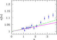
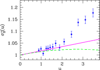
Figure 1: $\sigma^{+}_{\rm VA+AV}(u)$ (schemes I and II): LO running (continuous line), NLO running (dashed line) and NP data (points) from [2].

We conclude that the SF scheme has to be chosen with care in order to achieve a good control of the matching to the continuum schemes.

References

• [1]
• [2] M. Guagnelli et al. [ALPHA Collaboration], Nucl. Phys. Proc. Suppl.  119 (2003) 436
• [3] R. Frezzotti et al. [ALPHA Collaboration], JHEP 0108 (2001) 058
• [4] S. Sint and P. Weisz, Nucl. Phys. B 502 (1997) 251
• [5] G. Altarelli, G. Curci, G. Martinelli and S. Petrarca, Nucl. Phys. B 187 (1981) 461.
• [6] G. Martinelli, Phys. Lett. B 141 (1984) 395.
• [7] R. Frezzotti et al., Nucl. Phys. B 373 (1992) 781.
• [8] S. Sint and R. Sommer, Nucl. Phys. B 465 (1996) 71