Momentum dependence of the N to $\Delta$ transition form factors

Abstract

We present a new method to determine the momentum dependence of the N to $\Delta$ transition form factors and demonstrate its effectiveness in the quenched theory at $\beta=6.0$ on a $32^{3}\times 64$ lattice. We address a number of technical issues such as the optimal combination of matrix elements and the simultaneous overconstrained analysis of all lattice vector momenta contributing to a given momentum transfer squared, $Q^{2}$.

1 Introduction

The N to $\Delta$ transition form factors encode important information on hadron deformation and have been studied carefully in recent experiments [2]. In this work we present the first lattice evaluation of the momentum dependence of the magnetic dipole, M1, the electric quadrupole, E2, and the Coulomb quadrupole, C2, transition amplitudes. They are calculated in the quenched approximation on a lattice of size $32^{3}\times 64$ at $\beta=6.0$ with Wilson fermions with sufficient accuracy to exclude a zero value of E2 and C2 at low $Q^{2}$. This accuracy is achieved by applying two novel methods: 1) We use an interpolating field for the $\Delta$ that allows a maximum number of statistically distinct lattice measurements contributing to a given $Q^{2}$. 2) We extract the transition form factors by performing an overconstrained analysis of the lattice measurements using all lattice momentum vectors contributing to a given $Q^{2}$ value  [3].

2 Evaluation of the three-point function

The evaluation of the three-point function $G^{\Delta j^{\mu}N}_{\sigma}(t_{2},t_{1};{\bf p}^{\;\prime},{\bf p};\Gamma)$ can be done either using the fixed current approach as in previous lattice calculations [4, 5] or the fixed sink approach, where the current can couple to the backward sequential propagator at any time slice $t_{1}$ carrying any lattice momentum [6], allowing the evaluation of the form factors at all possible momentum transfers. As shown in Fig. 1, for the same statistics, the errors in M1 in the fixed sink method are almost three times as large as those obtained in the fixed current approach. Therefore in order to make use of the advantages of the fixed sink approach, we must first reduce the errors. We start by modifying the ratio used in ref. [5] so that we do not need to evaluate both $\langle G^{\Delta j^{\mu}N}_{\sigma}(t_{2},t_{1};{\bf p}^{\;\prime},{\bf p};\Gamma)\rangle$ and $\langle G^{Nj^{\mu}\Delta}_{\sigma}(t_{2},t_{1};{\bf p}^{\;\prime},{\bf p};\Gamma)\rangle$, since this would require two inversions. Instead we use the ratio

$$R_{\sigma}=\frac{\langle G^{\Delta j^{\mu}N}_{\sigma}(t_{2},t_{1};{\bf p}^{\;\prime},{\bf p};\Gamma)\rangle\;}{\langle G^{\Delta\Delta}_{ii}(t_{2},{\bf p}^{\;\prime};\Gamma_{4})\rangle\;}\biggr{[}\frac{\langle G^{\Delta\Delta}_{ii}(t_{2},{\bf p}^{\;\prime};\Gamma_{4})\rangle}{\langle G^{NN}(t_{2},{\bf p};\Gamma_{4})\rangle}\>$$ (1)

$$\hskip 5.69046pt\frac{\langle G^{NN}(t_{2}-t_{1},{\bf p};\Gamma_{4})\rangle\;\langle G^{\Delta\Delta}_{ii}(t_{1},{\bf p}^{\;\prime};\Gamma_{4})\rangle}{\langle G^{\Delta\Delta}_{ii}(t_{2}-t_{1},{\bf p}^{\;\prime};\Gamma_{4})\rangle\;\langle G^{NN}(t_{1},{\bf p};\Gamma_{4})\rangle}\biggr{]}^{1/2}$$

$$\hskip 34.14322pt\stackrel{{\scriptstyle t_{2}-t_{1}\gg 1,t_{1}\gg 1}}{{\Rightarrow}}\Pi_{\sigma}({\bf p}^{\;\prime},{\bf p}\;;\Gamma;\mu)\;,$$

in the notation of ref. [5]. We use kinematics where the $\Delta$ is produced at rest and so ${\bf q}\equiv{\bf p}^{\prime}-{\bf p}=-{\bf p}$. We fix $t_{2}/a=12$ and search for a plateau of $R_{\sigma}(t_{2},t_{1};{\bf p}^{\;\prime},{\bf p}\;;\Gamma;\mu)$ as function of $t_{1}$.

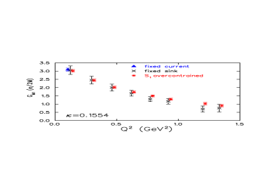
Figure 1: ${\cal G}_{M1}$ in Bohr magnetons at $\kappa=0.1554$.

In the fixed sink approach, the index $\sigma$ of the $\Delta$ and projection matrix $\Gamma$ are fixed and therefore we need to determine the most suitable choice of three-point functions from which to extract the Sachs form factors ${\cal G}_{M1},{\cal G}_{E2}$ and ${\cal G}_{C2}$ [5]. For example ${\cal G}_{M1}$ can be extracted from

$$\Pi_{\sigma}({\bf q}\;;\Gamma_{4};\mu)=iA\epsilon^{\sigma 4\mu j}p^{j}{\cal G}_{M1}(Q^{2})$$ (2)

where $A$ is a kinematical coefficient and $\Gamma=\Gamma_{4}=\frac{1}{2}\left(\begin{array}[]{cc}I&0\\ 0&0\end{array}\right)$ in Eq. (1). This leaves 3 choices for $\sigma$ i.e there are three statistically independent matrix elements yielding ${\cal G}_{M1}$, each requiring a sequential inversion. However, due to the $\epsilon$ factor, fixing $\sigma$ means that only momentum transfers in the other two directions contribute. Instead, if we take the symmetric combination, $S_{1}({\bf q};\mu)=\sum_{\sigma=1}^{3}\Pi_{\sigma}({\bf q};\Gamma_{4};\mu),$ momentum vectors in all directions contribute. This combination, which we refer to as sink $S_{1}$, is built into the $\Delta$ interpolating field and requires only one inversion. To take full advantage of the number of lattice vectors contributing to a given $Q^{2}$ we perform an overconstrained fit by solving the overcomplete set of equations $P({\bf q};\mu)=D({\bf q};\mu)\cdot F(Q^{2})$ where $P({\bf q};\mu)$ are the lattice measurements of the ratio of Eq. (1), $F=\left(\begin{array}[]{c}{\cal G}_{M1}\\ {\cal G}_{E2}\\ {\cal G}_{C2}\end{array}\right)$ and, with $N$ being the number of current directions and momentum vectors contributing to a given $Q^{2}$, D is an $N\times 3$ matrix which depends on kinematical factors. We extract the form factors by minimizing $\chi^{2}=\sum_{k=1}^{N}\frac{1}{w_{k}^{2}}\left(\sum_{j=1}^{3}D_{kj}F_{j}-P_{k}\right)^{2},$ where $w_{k}$ are the errors in the lattice measurements, using singular value decomposition of D. In Fig. 1, we compare the results for ${\cal G}_{M1}$ using an overconstrained analysis with sink type $S_{1}$ to our old analysis with fixed $\sigma=2$ and $\mu=3$. The errors with our new analysis are reduced at all values of $Q^{2}$ and are now equal to the error obtained using the fixed current approach.

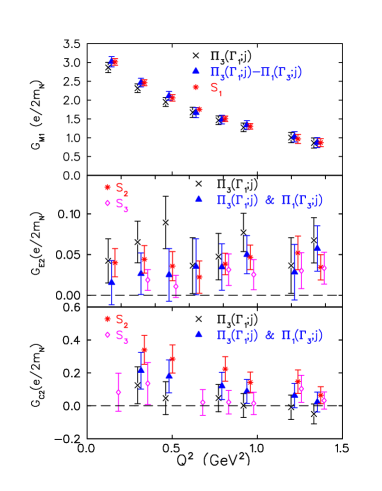
Figure 2: Top: ${\cal G}_{M1}$, middle: ${\cal G}_{E2}$, bottom: ${\cal G}_{C2}$ in Bohr magnetons at $\kappa=0.1554$ using $\Pi_{3}({\bf q};\Gamma_{1};j)$ (crosses), $\Pi_{3}({\bf q};\Gamma_{1};j)$ & $\Pi_{1}({\bf q};\Gamma_{3};j)$ (filled triangles), $S_{1}$ or $S_{2}$ (asterisks) and $S_{3}$ (open circles) and an overconstrained analysis.

Using $\Gamma_{k}=\frac{1}{2}\left(\begin{array}[]{cc}\sigma_{k}&0\\ 0&0\end{array}\right)$ instead of $\Gamma_{4}$ gives another six statistically independent 3-point functions from which ${\cal G}_{M1}$ can be extracted:

$$\vspace*{-0.5cm}\Pi_{\sigma}({\bf q}\;;\Gamma_{k};j) = B\Biggl{\{}\frac{1}{2}\left(p_{\sigma}\delta_{kj}-p_{k}\delta_{\sigma j}\right){\cal G}_{M1}(Q^{2})$$ (3)

$$-\biggl{[}\frac{3}{2}\left(p_{\sigma}\delta_{kj}+p_{k}\delta_{\sigma j}\right)-\frac{3p_{\sigma}p_{k}p_{j}}{{\bf p}^{2}}\biggr{]}{\cal G}_{E2}(Q^{2})$$

$$-\frac{(E_{N}-m_{\Delta})}{2m_{\Delta}}\>p_{j}\>\biggl{(}\delta_{\sigma k}-\frac{3p_{\sigma}p_{k}}{{\bf p}^{2}}\biggr{)}{\cal G}_{C2}(Q^{2})\Biggr{\}}$$

where $B$ and $C$ are kinematical coefficients. To isolate the benefits of using $S_{1}$ we compare in Fig. 2 ${\cal G}_{M1}$ obtained using $S_{1}$ to the the ones obtained by fixing $\sigma=3$ and $\Gamma_{1}$ in Eq. (3) [5]. All results are now obtained with the overconstrained analysis using 50 configurations. As can be seen, $S_{1}$ produces results with the smallest errors and it is therefore the optimal sink for ${\cal G}_{M1}$.

For the extraction of the quadrupole moments, we consider the symmetric combination $S_{2}({\bf q};\mu)=\sum_{\sigma\neq k=1}^{3}\Pi_{\sigma}({\bf q};\Gamma_{k};\mu)$ from which both ${\cal G}_{E2}$ and ${\cal G}_{C2}$ can be extracted when the current is in the spatial direction. When the current is in the time direction, $S_{2}$ provides a statistically independent way for evaluating ${\cal G}_{C2}$, at no extra cost. Another combination to extract the quadrupole form factors is $S_{3}=\Pi_{3}({\bf q}\;;\Gamma_{3};\mu)-\frac{1}{2}\bigl{(}\Pi_{1}({\bf q}\;;\Gamma_{1};\mu)+\Pi_{2}({\bf q}\;;\Gamma_{2};\mu)\bigr{)},$which, unlike $S_{2}$, contributes at the lowest value of $Q^{2}$. As can be seen in Fig. 2, $S_{2}$ produces results with smaller errors as compared to those using $\Pi_{3}(\Gamma_{1};j)$ and $\Pi_{1}(\Gamma_{3};j)$ for both E2 and C2. Increasing the the statistics from 50 to 200 configurations brings agreement between $S_{2}$ and $S_{3}$ for ${\cal G}_{C2}$ as well.

3 Results and Conclusions

We analyse 200 configurations at $\kappa=0.1554,$ 0.1558 and 0.1562 corresponding to $m_{\pi}/m_{\rho}=0.64,$ 0.59 and $0.50$ respectively. We use the nucleon mass at the chiral limit to set the lattice spacing $a$, obtaining $a^{-1}=2.04(2)$ GeV. Using the optimal sink $S_{1}$ our results for ${\cal G}_{M1}^{*}$ are shown in Fig. 3 as a function of $Q^{2}$, where

$$\vspace*{-0.3cm}{\cal G}_{M1}^{*}\equiv\frac{1}{3}\>\frac{1}{\sqrt{1+\frac{Q^{2}}{(m_{N}+m_{\Delta})^{2}}}}\>{\cal G}_{M1}\quad.\vspace*{-0.3cm}$$ (4)

Results in the chiral limit are obtained by performing a linear extrapolation in $m_{\pi}^{2}$. On the same figure, we also show the experimental values as extracted from the measured cross sections using the phenomenological model MAID [7]. Although the lattice data in the chiral limit lie higher than the MAID data both data sets are well described by the the phenomenological parametrization ${\cal G}_{a}(Q^{2})={\cal G}_{a}(0)\left(1+\alpha Q^{2}\right)\exp(-\gamma Q^{2})G_{E}^{p}(Q^{2})$ for $a=M1,E2$ and $C2$ and $G_{E}^{p}(Q^{2})=1/(1+Q^{2}/0.71)^{2}$ is the proton electric form factor. These fits are shown in Fig. 3 by the solid lines.

In Fig. 3, we show the ratios ${\rm EMR}\equiv R_{EM}=-\frac{{\cal G}_{E2}(q^{2})}{{\cal G}_{M1}(q^{2})}$ and ${\rm CMR}\equiv R_{SM}=-\frac{|{\bf q}|}{2m_{\Delta}}\;\frac{{\cal G}_{C2}(q^{2})}{{\cal G}_{M1}(q^{2})}$. Results in the chiral limit are obtained by performing a linear extrapolation in $m_{\pi}^{2}$. As expected, both EMR and CMR become more negative as we approach the chiral limit. The results for EMR are in agreement with experimental measurements whereas CMR is not as negative as experiment at low $Q^{2}$. We believe that CMR is particularly sensitive to the absence of sea quarks and thus a good probe of unquenching effects.

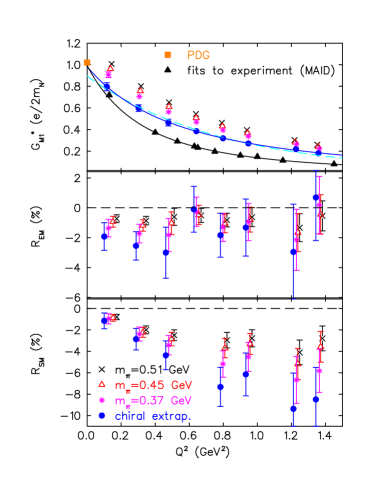
Figure 3: Top: ${\cal G}_{M1}^{*}$, middle: EMR, bottom: CMR as function of $Q^{2}$ at $\kappa=0.1554$ (crosses), $\kappa=0.1558$ (open triangles), $\kappa=0.1562$ (asterisks) and in the chiral limit (filled circles). Filled triangles show ${\cal G}_{M1}^{*}$ extracted from measurements using MAID [7]. The dashed line is a fit to the lattice data using $a\exp(-bQ^{2})$.

References

- [1]
- [2] C.Mertz et al., Phys. Rev. Lett. 86, 2963 (2001); K. Joo et al., Phys. Rev. Lett. 88 122001 (2002).
- [3] LHPC and SESAM collaborations, Ph. Hägler, et. al, Phys. Rev. D68, 034505 (2003).
- [4] D. B. Leinweber, T. Draper, and R. M. Woloshyn, Phys. Rev. D 48, 2230 (1993).
- [5] C. Alexandrou, et. al, Phys. Rev. D 69, 114506 (2004).
- [6] C. Alexandrou, et. al, Nucl. Phys. (Proc. Suppl.) 129, 221 (2004); C.Alexandrou, Nucl. Phys. (Proc. Suppl.) 128, 1 (2004).
- [7] D. Drechsel, O. Hanstein, S.S. Kamalov and L. Tiator, Nucl. Phys. A645 145 (1999).