Numerical Study of Lattice Landau Gauge QCD
and the Gribov Copy Problem

Abstract

The infrared properties of lattice Landau gauge QCD of SU(3) are studied by measuring gluon propagator, ghost propagator, QCD running coupling and Kugo-Ojima parameter of $\beta=6.0,16^{4},24^{4},32^{4}$ and $\beta=6.4,32^{4},48^{4},56^{4}$ lattices. By the larger lattice measurements, we observe that the runnning coupling measured by the product of the gluon dressing function and the ghost dressing function squared rescaled to the perturbative QCD results near the highest lattice momentum has the maximum of about 2.2 at around $q=0.5$ GeV/c, and behaves either approaching constant or even decreasing as $q$ approaches zero. The magnitude of the Kugo-Ojima parameter is getting larger but staying around $-0.83$ in contrast to the expected value $-1$ in the continuum theory. We observe, however, there is an exceptional sample which has larger magnitude of the Kugo-Ojima parameter and stronger infrared singularity of the ghost propagator. The reflection positivity of the 1-d Fourier transform of the gluon propagator of the exceptional sample is manifestly violated.

Gribov noise problem was studied by performing the fundamental modular gauge (FMG) fixing with use of the parallel tempering method of $\beta=2.2,16^{4}$ SU(2) configurations. Findings are that the gluon propagator almost does not suffer noises, but the Kugo-Ojima parameter and the ghost propagator in the FMG becomes $\sim 5$% less in the infrared region than those suffering noises. It is expected that these qualitative aspects seen in SU(2) will reflect in the infrared properties of SU(3) QCD as well.

1 Introduction

One of our basic motivations in the present study is verification of the color confinement mechanism in the Landau gauge. Two decades ago, Kugo and Ojima proposed a criterion for the color confinement in Landau gauge QCD using the Becchi-Rouet-Stora-Tyutin(BRST) invariance of continuum theory [1]. Gribov pointed out that the Landau gauge can not be uniquely fixed, that is, the Gribov copy problem, and argued that the unique choice of the gauge copy could be a cause of the color confinement [2]. Later Zwanziger developed extensively the lattice Landau gauge formulation [3] in view of the Gribov copy problem. Kugo and Ojima started from naive Faddeev-Popov Lagrangian obviously ignoring the Gribov copy problem, and gave the color confinement criterion with use of the following two point function of the covariant derivative of the ghost and the commutator of the antighost and gauge field:

$$(\delta_{\mu\nu}-{q_{\mu}q_{\nu}\over q^{2}})u^{ab}(q^{2})\qquad\qquad\qquad\qquad\qquad\qquad$$

$$={1\over V}\sum_{x,y}e^{-ip(x-y)}\langle{\rm tr}\left({\lambda^{a}}^{{\dagger}}D_{\mu}\displaystyle{1\over-\partial D}[A_{\nu},\lambda^{b}]\right)_{xy}\rangle$$ , (1)

where lattice simulation counterpart is utilized. They claim that sufficient condition of the color confinement is that $u(0)=-1$ with $u^{ab}(0)=\delta^{ab}u(0)$. Kugo showed that

$$1+u(0)=\frac{Z_{1}}{Z_{3}}=\frac{\tilde{Z}_{1}}{\tilde{Z}_{3}},$$ (2)

where $Z_{3}$ is the gluon wave function renormalization factor, $Z_{1}$ is the gluon vertex renormalization factor, and $\tilde{Z}_{3}$ is the ghost wave function renormalization factor, respectively. In the continuum theory $\tilde{Z}_{1}$ is a constant in perturbation theory and is set to be 1. On the lattice, it is not evident that it remains 1 when strong non-perturbative effects are present. In a recent SU(2) lattice simulation with several values of $\beta$, finiteness of $\tilde{Z}_{1}$ seems to be confirmed, but its value differ from 1.

The same equality, the first one of equations (2), was derived by Zwanziger with use of his ”horizon condition” about the same time [3]. It is to be noted that arguments of both Kugo and Zwanziger are perturbative ones in that they used diagramatic expansion, and the equation (2) is of continuum theory or continuum limit.

The non-perturbative color confinement mechanism was studied with the Dyson-Schwinger approach [4, 5] and lattice simulations [6, 7, 8, 9, 10]. Both types of studies are complementary in that Dyson-Schwinger approach needs ansatz for truncation of interaction kernels and lattice simulation is hard to draw conclusions of continuum limit although the calculation is one from the first principle.

We measured in SU(3) lattice Landau gauge simulation with use of two options of gauge field definition ($\log U$, $U$ linear; see below), gluon propagator, ghost propagator, QCD running coupling and Kugo-Ojima parameter of $\beta=6.0,16^{4},24^{4},32^{4}$ and $\beta=6.4,32^{4},48^{4},56^{4}$ lattices. The QCD running coupling $\alpha_{s}=g^{2}/4\pi$ can be measured in terms of gluon dressing functiuon $Z(q^{2})$ and ghost dressing function $G(q^{2})$, as renormalization group invariant quatity $g^{2}G(q^{2})^{2}Z(q^{2})$. Infrared features of $g^{2}$ is not known, however, and there remains a problem of checking the Gribov noise effect among those quantities, since there exist no practical algorithms available so far for fixing fundamaental modular gauge (see below). In our $56^{4}$ simulation, we encountered a copy of an exceptional configuration yielding extraordinarily large Kugo-Ojima marameter $c=-u(0)$, and studied its feature in some more detail. We made another copy by adjusting controlling parameter in gauge fixing algorithm, and measured copywise 1-d FT of the gluon propagator, and found violation of reflection positivity in both cases.

In order to study the Gribov copy problem, we made use of parallel tempering [9] with 24 replicas to fix fundamental modular gauge in SU(2), $\beta=2.2,\ 16^{4}$ lattice, and obtained qualitatively similar result as Cucchieri[12].

1.1 The lattice Landau gauge

We adopt two types of the gauge field definitions:

1. $\log U$ type: $U_{x,\mu}=e^{A_{x,\mu}},\ A_{x,\mu}^{{\dagger}}=-A_{x,\mu},$

2. $U$ linear type: $A_{x,\mu}=\displaystyle{1\over 2}(U_{x,\mu}-U_{x,\mu}^{{\dagger}})|_{trlp.}$,

where _trlp. implies traceless part. The Landau gauge, $\partial A^{g}=0$ is specified as a stationary point of some optimizing functions $F_{U}(g)$ along gauge orbit where $g$ denotes gauge transformation, i.e., $\delta F_{U}(g)=0\ {\rm for\ any\ }\delta g.$

Here $F_{U}(g)$ for the two options are [10, 3]

1. $F_{U}(g)=||A^{g}||^{2}=\sum_{x,\mu}{\rm tr}\left({{A^{g}}_{x,\mu}}^{{\dagger}}A^{g}_{x,\mu}\right)$,

2. $F_{U}(g)=\sum_{x,\mu}\left(1-{1\over 3}{\rm Re}\ {\rm tr}U^{g}_{x,\mu}\right),$

respectively. Under infinitesimal gauge transformation $g^{-1}\delta g=\epsilon$, its variation reads for either defintion as

$$\Delta F_{U}(g)=-2\langle\partial A^{g}|\epsilon\rangle+\langle\epsilon|-\partial{D(U^{g})}|\epsilon\rangle+\cdots,$$

where the covariant derivativative $D_{\mu}(U)$ for two options reads commonly as
$D_{\mu}(U_{x,\mu})\phi=S(U_{x,\mu})\partial_{\mu}\phi+[A_{x,\mu},\bar{\phi}]$
where $\partial_{\mu}\phi=\phi(x+\mu)-\phi(x)$, and
$\bar{\phi}=\displaystyle{\phi(x+\mu)+\phi(x)\over 2}$, but definition of operation $S(U_{x,\mu})B_{x,\mu}$ is given

1. $$S(U_{x,\mu})B_{x,\mu}=T({\cal A}_{x,\mu})B_{x,\mu}$$ (3)

   where ${\cal A}_{x,\mu}=adj_{A_{x,\mu}}=[A_{x,\mu},\cdot]$,
   $T(x)=\displaystyle{{x/2\over{\rm th}(x/2)}}.$

2. $$S(U_{x,\mu})B_{x,\mu}=\displaystyle{1\over 2}\left.\left\{\displaystyle{U_{x,\mu}+U_{x,\mu}^{\dagger}\over 2},B_{x,\mu}\right\}\right|_{trlp.}$$ (4)

The fundamental modular gauge (FMG) [3] is specified by the global minimum of the minimizing function $F_{U}(g)$ along the gauge orbits in either case, i.e.,
$\Lambda=\{U|\ A=A(U),F_{U}(1)={\rm Min}_{g}F_{U}(g)\}$, $\Lambda\subset\Omega$, where $\Omega$ is Gribov region (local minima), and $\Omega=\{U|-\partial{D(U)}\geq 0\ ,\ \partial A=0\}.$

2 Numerical simulation of lattice Landau gauge QCD

2.1 Method of simulation

First we produce Monte Carlo (Boltzmann) samples of link variable configuration according to Wilson’s plaquette action by using the heat-bath method. We use optimally tuned combined algorithm of Creutz’s and Kennedy-Pendleton’s for SU(2) case, and Cabbibo -Marinari pseudo-heat-bath method with use of the above SU(2) algorithm for SU(3) case. As for FMG fixing, the smearing gauge fixing works well for large $\beta$ on relatively small size lattice [8]. However we found that its performance for SU(3), $\beta=6.0$, $16^{4}$ lattice is not perfect in comparison with our standard method for $\log U$ type definition, in which the third order perturbative treatment of the linear equation with respect to gauge field $A$, $-\partial D\epsilon=\partial A$ is performed. For $U$ linear definition, we use the standard overrelaxation method for both SU(2) and SU(3). Thus we know that our gauge fixing is not FMG fixng. The accuracy of $\partial A(U)=0$ is $10^{-4}$ in the maximum norm in all cases.

Measurement of quantity in question, gluon propagator, ghost propagator, Kugo-Ojima parameter, etc., is performed with use of Landau gauge fixed copy, and averaged over Monte Carlo samples.

We define the gluon dressing function $Z_{A}(q^{2})$ from the gluon propagator of SU($n$)

$$D_{\mu\nu}(q) = {1\over n^{2}-1}\sum_{x={\bf x},t}e^{-ikx}{\rm tr}\langle A_{\mu}(x)^{\dagger}A_{\nu}(0)\rangle$$ (5)

$$= (\delta_{\mu\nu}-{q_{\mu}q_{\nu}\over q^{2}})D_{A}(q^{2}),$$

as $Z_{A}(q^{2})=q^{2}D_{A}(q^{2})$.

The ghost propagator is defined as the Fourier transform of an expectation value of the inverse of Faddeev-Popov(FP) operator ${\cal M}=-\partial D$,

$$D_{G}^{ab}(x,y)=\langle{\rm tr}\langle{\lambda^{a}}_{x}|({\cal M}[U])^{-1}|{\lambda^{b}}_{y}\rangle\rangle,$$ (6)

where the outmost $\langle\cdots\rangle$ denotes average over samples $U$.

2.2 Numerical results of simulation

$D_{A}(q^{2})$ is defined in (5), and its dressing function is given as $Z_{A}(q^{2})=q^{2}D_{A}(q^{2})$.

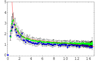
Figure 1: The gluon dressing function as the function of the momentum $q$(GeV). $\beta=6.4$, $48^{4}$(stars) and $56^{4}$(diamonds) in the $\log U$ definition. The solid line is that of the $\widetilde{\rm MOM}$ scheme.

Numerical results are given in figure.1.

The ghost propagator is defined in (6). It should be noted that the operator $[{\cal M}(U)]^{ab}_{xy}$ is a real symmetric operator when $\partial A=0$, and it transforms covariantly under global color gauge transformation $g$, i.e., $[{\cal M}(U^{g})]^{ab}=[g^{\dagger}\{{\cal M}(U)\}g]^{ab}$. The conjugate gradient method is used for the evaluation the ghost propagator, and absence of color off-diagonal components manifests itself, a signal of no color summetry violation in Landau gauge. The accuracy of the inversion is maintained less than 5% in maximum norm in error check of the source term.

We measured the running coupling from the product of the gluon dressing function and the ghost dressing function squared.

$$\alpha_{s}(q^{2})=\frac{g_{0}^{2}}{4\pi}Z(q^{2}){G(q^{2})}^{2}\simeq(qa)^{-2(\alpha_{D}+2\alpha_{G})}.$$ (7)

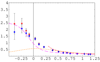
Figure 2: The running coupling $\alpha_{s}(q)$ as a function of the logarithm of momentum $\log_{10}q$(GeV) of the $\log U$, $\beta=6.4$, $56^{4}$ lattice using the ghost propagator of the average (diamond). The result using the ghost propagator of $I_{A}$ copy (star) is also plotted for comparison. The DSE approach (long dashed line), the perturbative QCD+$c/q^{2}$ (short dashed line) and the contour improved perturbation method (dotted line) are also shown.

The lattice data (diamonds) are compared with a fit of the DSE approach[5] with infrared fixed point $\alpha_{0}=2.5$, and the pertubative QCD with $c/q^{2}$ correction [7] and the contour improved perturbation method[10]. The The result using the ghost propagator of $I_{A}$ copy (star) is also plotted for presenting the ambiguity due to the Gribov copy.

Kugo-Ojima color confinement criterion is given with use of $u^{ab}(p^{2})$ defined in (1) with $u^{ab}(p^{2})=\delta^{ab}u(p^{2})$, as $u(0)=-c;\ c=1\to{\rm color\ confinement}$. Zwanziger’s horizon condition [3] derived in the infinite volume limit is written as follows;

$$\sum_{x,y}e^{-ip(x-y)}\left\langle{\rm tr}\left({\lambda^{a}}^{{\dagger}}D_{\mu}\displaystyle{1\over-\partial D}(-D_{\nu})\lambda^{b}\right)_{xy}\right\rangle$$

$$=G_{\mu\nu}(p)\delta^{ab}=\left(\displaystyle{e\over d}\right)\displaystyle{p_{\mu}p_{\nu}\over p^{2}}\delta^{ab}-\left(\delta_{\mu\nu}-\displaystyle{p_{\mu}p_{\nu}\over p^{2}}\right)u^{ab},$$

where $e=\left\langle\sum_{x,\mu}{\rm tr}(\lambda^{a{\dagger}}S(U_{x,\mu})\lambda^{a})\right\rangle/\{(n^{2}-1)V\}$, and the horizon condition reads $\displaystyle\lim_{p\to 0}G_{\mu\mu}(p)-e=0$, and the l.h.s. of the condition is $\left(\displaystyle{e\over d}\right)+(d-1)c-e=(d-1)h$ where $h=c-\displaystyle{e\over d}$ and dimension $d=4$, and it follows that $h=0\to{\rm horizon\ condition}$, and thus the horizon condition coincides with Kugo-Ojima criterion provided the covariant derivative approaches the naive continuum limit, i.e., $e/d=1$.
Values of $\displaystyle c,\frac{e}{d},h$ are shown in the Table 1.(suffix 1: $\log U$, suffix 2: $U-$linear)

Table 1: The Kugo-Ojima parameter $c$ in $\log U$ and $U-$linear version. $\beta=6.0$ and $6.4$.

$\beta$	$L$	$c_{1}$	$e_{1}/d$	$h_{1}$	$c_{2}$	$e_{2}/d$	$h_{2}$
6.0	16	0.628(94)	0.943(1)	-0.32(9)	0.576(79)	0.860(1)	-0.28(8)
6.0	24	0.774(76)	0.944(1)	-0.17(8)	0.695(63)	0.861(1)	-0.17(6)
6.0	32	0.777(46)	0.944(1)	-0.16(5)	0.706(39)	0.862(1)	-0.15(4)
6.4	32	0.700(42)	0.953(1)	-0.25(4)	0.650(39)	0.883(1)	-0.23(4)
6.4	48	0.793(61)	0.954(1)	-0.16(6)	0.739(65)	0.884(1)	-0.15(7)
6.4	56	0.827(27)	0.954(1)	-0.12(3)	0.758(52)	0.884(1)	-0.13(5)

Among gauge fixed configurations, $\beta=6.4$, $\log U$ type, there appeared a configuration ($I_{A}$) which have exceptionally large Kugo-Ojima parameters, $c=0.851(77)$ with rather large fluctuation among diagonal components. For more informtion, we made another copy of it by changing some parameter of the gauge fixing program. They have very close values in $\|A\|^{2}$ norm, but fairly large difference in physically important values. One dimensional Fourier transforms transverse to 4 axes were calculated with respect to sample-wise transverse gluon propagator functions of momentum $q$. Existence of negative value region in one dimensional Fourier tranform of (sample averaged) propagator implies violation of reflection positivity postulate[11].

3 The Gribov copy problem

The Gribov copy problem is one of fundamental problems in QCD. FMG is the unique gauge known as the legitimate Landau gauge without Gribov copies. No algorithms for FMG fixing have been established. Numerical invesigations of Gribov noise have been done in a few works [12]. For $U$ linear type gauge field definition, FMG gauge fixing with use of parallel tempering (PT) with 24 replicas was performed for $\beta=2.2,16^{4}$, SU(2) 67 Monte Carlo configurations. Some more details of the method are given in [9]. We compared data between two groups, the absolute minimum configurations of $F_{U}(g)$ obtained by Landau gauge fixing via PT and the 1st copies obtained by the direct application of Landau gauge fixing on Monte Carlo configurations. The results are as follows; 1)The singularity of the ghost propagator of the FMG is about 6% less than that of the 1st copy. 2)Kugo-Ojima parameter $c$ of the FMG is about 4% smaller than that of the 1st copy. 3) The gluon propagator of the two groups are almost the same within statistical errors. 4) The running coupling of FMG is about 10% suppressed than that of the 1st copy. 5) The horizon function deviation parameter $h$ of the FMG is not closer to 0, i.e. the value expected in the continuum limit, than that of the 1st copy.

In Fig.3, shown is the scatter plot of Gribov copies on the plane of Kugo-Ojima parameter vs $1-F_{U}(g)$, 32 copies via random gauge transformation and one copy given via PT, all being Gribov copies on a single gauge orbit.

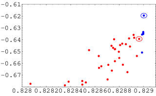
Figure 3: The Kugo-Ojima parameter $u(0)$ vs $1-F_{U}(g)$ of the 33 copies on a single gauge orbit. $SU(2)$, @$\beta=2.2$, $16^{4}$. The maximum optimization point by Cucchieri’s prescription(lower circle) and our prescription(upper circle) are indicated.

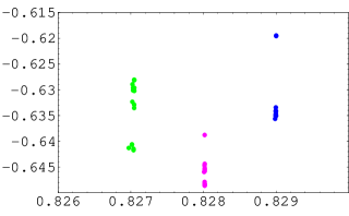
Figure 4: The Kugo-Ojima parameter $u(0)$ vs $1-F_{U}(g)$ of 16 Gribov copies via PT for three gauge orbits each.

In Fig.4, the best one of 16 copies should be picked up for the FMG. This figure shows how flat is the bottom of $F_{U}(g)$ with respect to the physical quantity.

4 Discussion and Conclusion

The SU(3) $\beta=6.0,16^{4},24^{4},32^{4}$ and $\beta=6.4,32^{4},48^{4},56^{4}$ lattice Landau gauge simulation was performed. A comparison of the data of $\log U$ type and the $U-$linear type reveals that the gluon propagator does not depend on the type and the ghost propagator of the $U-$linear is about 14% larger than the $\log U$. The Kugo-Ojima parameter $c$ is still getting larger $u(0)\sim-0.83$ in $\log U$ and about -0.76 in $U-$linear, in accordance to lattice size. The running coupling $\alpha_{s}(q)$ of the $\log U$ type has a maximum of about 2.2, and that of the $U-$linear is slightly smaller since they are rescaled at the high lattice momentum region. The absolute value of the index $\alpha_{G}$ increases as the lattice size becomes large but since it is defined at $q\sim 0.4GeV$ region, it is smaller than $\kappa\sim 0.5$ of the DSE which is defined at the 0 momentum region by about factor 2.

As is studied in SU(2) FMG data, the gluon propagator suffers almost no Gribov noise, but magnitude of Kugo-Ojima parameter becomes smaller in FMG, and the ghost propagator exhibits less singular infrared behavior in FMG than that supposed suffering noise. Accordingly the running coupling becomes smaller in FMG. All samples in SU(3) can not be supposed in FMG and supposed to suffer the Gribov noise, and it is expected that these qualitative aspects seen in SU(2) will reflect in the infrared behavior of SU(3) QCD as well. The FMG is mathematically well defined on lattice, and its existence can be proven. But rather flat valued feature of the FMG optimizing function with respect to physical quantities seem to keep annoying us, at least, technically, and this fact may suggest necessity of some new formulation of infrared dynamics of QCD. In the Langevin formulation of Landau gauge QCD, Zwanziger conjectured that the path integral over the FM region will become equivalent to that over the Gribov region in the continuum [13]. If his conjecture is correct, then in order for the gauge dependent quantity, e.g., the optimizing function to have the same expectation values on both regions, the situation that the probability density may be concentrated in some common local region becomes favorable one. The proximity of the FM region and the boundary of the Gribov region in SU(2) in $8^{4},12^{4}$ and $16^{4}$ lattices with $\beta=0,0.8,1.6$ and $2.7$ was studied in [14]. The tendency that the smallest eigenvalue of the Faddeev-Popov matrix of the FMG and that of the 1st copy come closer as $\beta$ and lattice size become larger was observed, although as remarked in [14] the physical volume of $\beta=2.7$, $16^{4}$ lattice is small and not close to the continuum limit. In this respect, further study of lattice size and $\beta$ dependence of Gribov noise of various quantities will become an important problem in future.

Our observation of exceptional configurations in SU(3), $\beta=6.4$, $56^{4}$ may be considered as a signal of the tendency of the probabililty concentration to the Gribov boundary[3, 11].

The confinement scenario was recently reviewed in the framework of the renormalization group equation and dispersion relation [15]. It is shown that the gluon dressing function satisfies the superconvergence relation, and the gluon propagator does not necessarily vanish as Gribov and Zwanziger conjectured, but it should be finite. The multiplicative renormalizable DSE approach[5] predicts that the exponent $\kappa=0.5$ and the infrared fixed point $\alpha_{0}=2.6$ and our lattice data are consistent with this prediction.

Acknowledgments:

We are grateful to Daniel Zwanziger for enlightning discussion. This work is supported by the KEK supercomputing project No. 03-94, and No. 04-106.

References

- [1] T. Kugo and I. Ojima, Prog. Theor. Phys. Suppl. 66, 1 (1979).
- [2] V.N. Gribov, Nucl. Phys. B 1391(1978).
- [3] D. Zwanziger, Nucl. Phys. B 364 ,127 (1991), idem B 412, 657 (1994).
- [4] L. von Smekal, A. Hauck, R. Alkofer, Ann. Phys. (N.Y.) 267,1 (1998).
- [5] J.C.R. Bloch, Few Body Syst 33,111(2003).
- [6] D.B. Leinweber et al., Phys. Rev. D60,094507(1999); ibid Phys. Rev. D61,079901(2000).
- [7] D. Becirevic et al., Phys. Rev. D 61,114508(2000).
- [8] H.Nakajima and S. Furui, Nucl. Phys. B (Proc Suppl.)73A-C,635, 865(1999) and references therein, Nucl. Phys. B (Proc Suppl.)83-84,521 (2000), 119,730(2003); Nucl. Phys. A 680,151c(2000).
- [9] H. Nakajima and S. Furui, Nucl. Phys. B(Proc. Supl.) 129-130(2004) and references therein, hep-lat/0309165.
- [10] S. Furui and H.Nakajima, Phys. Rev. D69,074505(2004) and references therein.
- [11] S. Furui and H.Nakajima, hep-lat/0403021 ver 3.
-
[12]
A.Cucchieri, Nucl. Phys. B508,353(1997),
hep-lat/9705005. - [13] D. Zwanziger, Phys. Rev. D69,016002(2004), hep-ph/0303028.
- [14] A. Cucchieri, Nucl. Phys. B521,365(1998), hep-lat/9711024.
- [15] K.I. Kondo, hep-th/0303251.