QCD thermodynamics from an Imaginary $\mu_{B}$:
results on the four flavor lattice model

Abstract

We study four flavor QCD at nonzero temperature and density by analytic continuation from an imaginary chemical potential. The explored region is $T=0.95T_{c}<T<3.5T_{c}$, and the baryochemical potentials range from 0 to $\simeq 500$ MeV. Observables include the number density, the order parameter for chiral symmetry, and the pressure, which is calculated via an integral method at fixed temperature and quark mass. The simulations are carried out on a $16^{3}\times 4$ lattice, and the mass dependence of the results is estimated by exploiting the Maxwell relations. In the hadronic region we confirm that the results are consistent with a simple resonance hadron gas model, and we estimate the critical density by combining the results for the number density with those for the critical line. In the hot phase, above the endpoint of the Roberge-Weiss transition $T_{E}\simeq 1.1T_{c}$ the results are consistent with a free lattice model with a fixed effective number of flavor slightly different from four. We confirm that confinement and chiral symmetry are coincident by a further analysis of the critical line, and we discuss the interrelation between thermodynamics and critical behavior. We comment on the strength and weakness of the method, and propose further developments.

I Introduction

QCD at nonzero temperature and density is an important subject both from a theoretical and phenomenological perspectiveKogutStephanov . Current and future experiments at RHIC and LHC will explore the region of the phase diagram close to the zero density axis, not far from the cooling path of the primordial universe. The cold, high density phases are relevant for astrophysics. Future GSI experiments might bridge these two regimes and explore the region of intermediate temperatures and densities.

While many predictions on the structure of the phase diagram can be obtained by use of simple models dictated by symmetry arguments, quantitative studies require a first principle calculation. Lattice field theory is the natural approach, and QCD at nonzero temperature and density is by now studied by a variety of lattice methods: the multiparameter reweighting method achieves on optimal overlap between the simulation ensemble at zero baryon density and the target ensemble at nonzero density Fodor:2001au ; Fodor:2002km ; Fodor:2001pe ; Fodor:2004nz ; the direct calculation of the derivatives gave the first informations on the physics at nonzero chemical potential Gavai:2003mf ; Gavai:2003nn ; deForcrand:2002pa ; the Taylor expanded reweighting reduces the numerical costs associated with the multiparameter reweighting Allton:2002zi ; Allton:2003vx ; the analytic continuation from an imaginary chemical potential uses the information from the $\mu^{2}\leq 0$ halfplane to reconstruct the physics of real baryon density Lombardo:1999cz ; Hart:2000ef ; deForcrand:2002ci ; D'Elia:2002gd ; deForcrand:2003hx . In addition to these pragmatic works, which take advantage of the fluctuations close to $T_{c}$ to explore the small chemical potential region $\mu/T\leq 1.$, there have been a number of new proposals Ambjorn:2002pz ; Azcoiti:2003vv ; Crompton:2001ws , discussionsEjiri:2004yw and checksGiudice:2004se . For recent reviews see Laermann:2003cv ; Katz:2003up , and for introductions into the subject see Muroya:2003qs ; Lombardo:2004uy .

In this paper we extend our study of four flavor QCD within the imaginary chemical potential approach. Let us remind that four flavor QCD has a first order transition at $\mu=0$, as it is the one at $T=0$. Hence, it is expected to have a first order critical line in the plane $T,\mu$: there is no tricritical point or endpoint to be investigated here. On the other hand, the first order (or sharp crossover) nature of the critical line makes the model simpler, and amenable to a detailed study with comparatively modest numerical resources.

In our first paper D'Elia:2002gd we studied the order parameter in the hadronic phase and calculated the critical line up to $\mu\simeq 500MeV$. We have indeed confirmed the expected first order (or very sharp crossover) nature of the transition, we have observed its interrelation with deconfinement, and we have studied its $N_{f}$ scaling by comparing our results with those of ref. deForcrand:2002ci . The results on the chiral condensate were consistent with a partition function described by a simple hyperbolic cosine behavior. Consistent numerical findings were reported in ref. Karsch:2003zq , and intepreted within a resonance gas model.

This work addresses more fully the properties of the hadronic phase, and those of the plasma phase. We base our analysis mostly on the results for the number density and for the chiral condensate. We calculate the subtracted pressure by an integral method at constant temperature and quark mass, and we study the mass dependence by taking numerical derivatives of the chiral condensate.

The properties of the quark gluon plasma phase are studied by means of the number density and of the subtracted pressure. We discuss the nonperturbative nature of the hot phase in the vicinity of the critical point, and we argue that this result follows naturally by an analysis of the phase diagram in the $T,\mu^{2}$ plane. We compare the numerical results with analytic predictions, a task for which the imaginary chemical potential approach is ideally suited: for instance, rather than analytically continue the numerical results to real chemical potential, we can continue the analytic predictions to the negative $\mu^{2}$ halfplane, and contrast the results with the numerical ones.

In the hadronic phase we study in detail the number density: its simple behavior will further support the applicability of the hadron resonance gas model; moreover we combine the results for the critical line with those for the number density in order to estimate the critical density.

In both phases we exploit the Maxwell relations to study the mass dependence: this turns out to be sizable in the hadronic phase, and negligible in the plasma phase.

Concerning the critical line, as already mentioned, the four flavor model has a first order transition. Hence, tricritical points or endpoints are not present here, and we contented ourselves with the precision reached in our previous study. The new results on the critical behavior consists in a more detailed analysis of the correlation of the chiral and the deconfinement transition.

The paper is organised as follows. In Section II we review the properties of the phase diagram of QCD in the chemical potential– temperature plane, including the new results on the critical behavior at a selected $\mu$ value. In Section III we describe our observables and give an overview of the results. Section IV is devoted to the results in the hadronic region, while Section V presents results for the Quark Gluon Plasma phase. In either phases we will discuss in detail the various ansätze which emerge naturally once the analyticity properties and the nature of the critical lines are taken into account. In Section VI we discuss our results for $T_{c}<T<T_{E}$ and give some general comment about this intermediate region of temperatures. We summarize and discuss future perspectives in Section VII. Some preliminary results have already appeared in D'Elia:2003uy .

II QCD in the $\mu^{2},T$ plane

Results from simulations with an imaginary chemical potential can be analytically continued to a real chemical potential, thus circumventing the sign problem Hart:2000ef ; deForcrand:2002ci ; D'Elia:2002gd . In practice, the analytical continuation is carried out along one line in the complex $\mu$ plane: first along the imaginary axes, and then along the real one. It is then meaningful to map this path in the complex $\mu^{2}$ plane: because of the symmetry property $Z(\mu)=Z(-\mu)$ this can be achieved without losing generality. In the complex $\mu^{2}$ plane the partition function is real for real values of the external parameter $\mu^{2}$, complex otherwise: the situation resembles that of ordinary statistical models in an external field. Hence, the analyticity of the physical observables Lombardo:1999cz as well as that of the critical line deForcrand:2002ci follows naturally.

The reality region for the partition function represents states which are physically accessible. The reality region for the determinant represents the region which is amenable to an importance sampling calculation: $\Re e\mu^{2}\leq 0$.

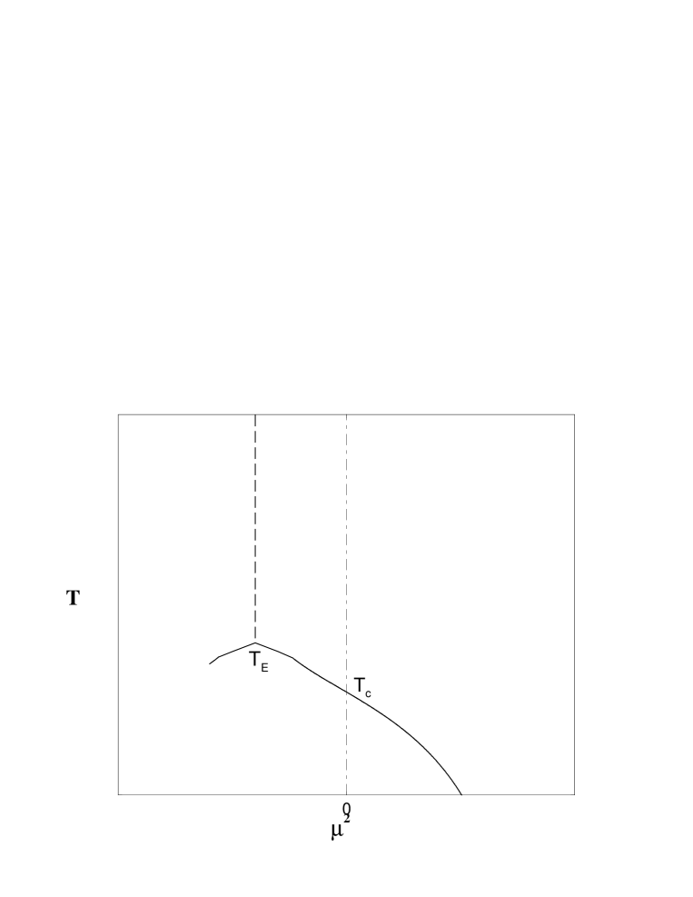
Figure 1: Sketch of the phase diagram in the $\mu^{2},T$ plane: the solid line is the chiral transition, the dashed line is the Roberge Weiss transition. Simulations can be carried out at $\mu^{2}\leq 0$ and results continued to the physical domain $\mu^{2}\geq 0$. The derivative and reweighting methods have been used so far to extract informations from simulations performed at $\mu=0.$ The imaginary chemical potential approaches uses results on the left hand half plane. Different methods could be combined to improve the overall performance

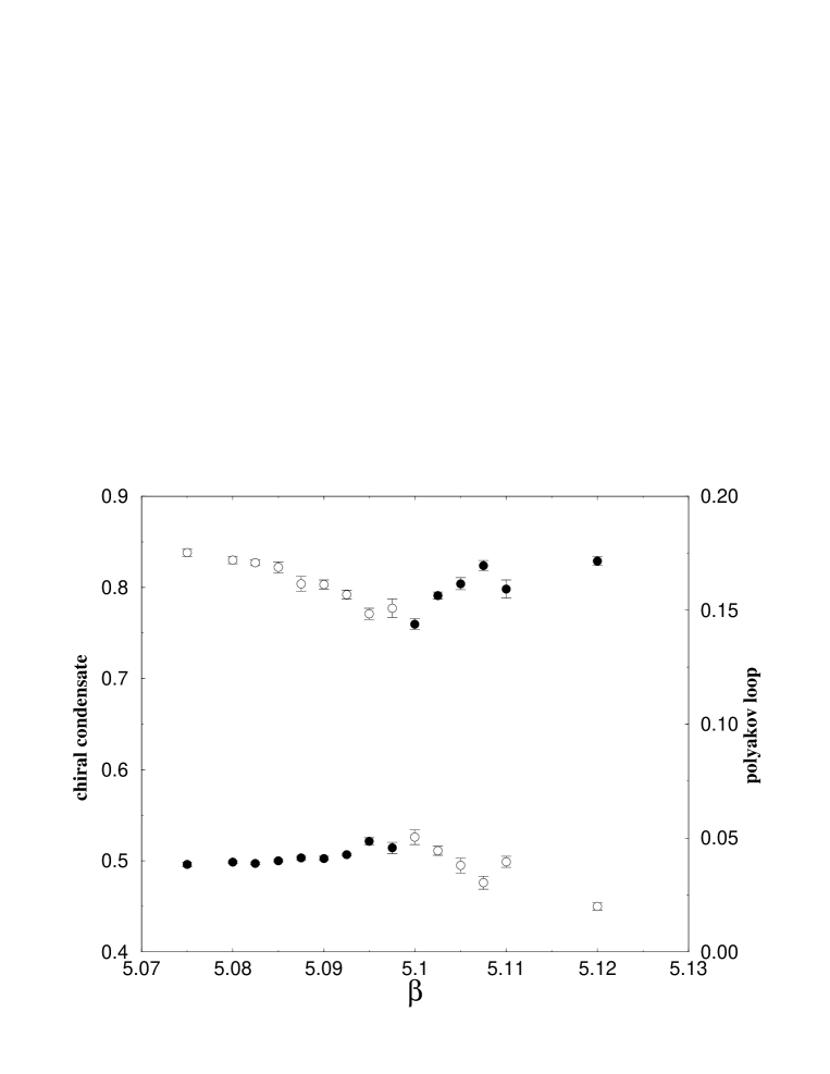
Figure 2: Correlation between $\langle\bar{\psi}\psi\rangle$ and Polyakov loop at $\mu_{I}=0.15$, demonstrating the correlation of chiral and deconfining transition at nonzero baryon density.

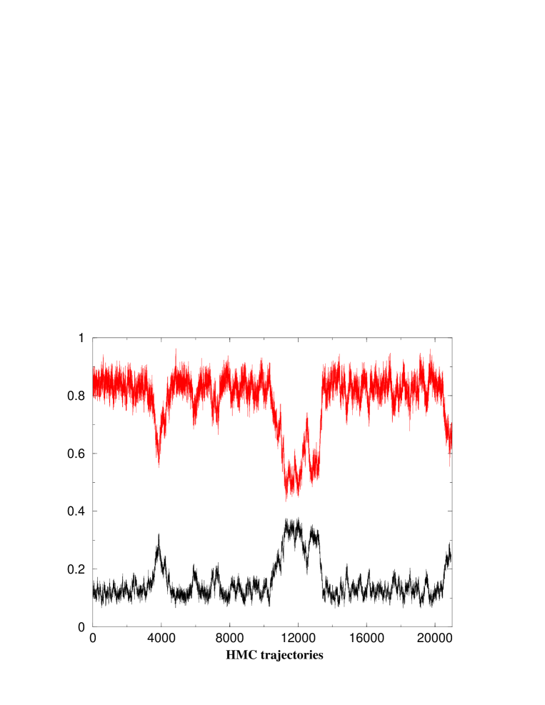
Figure 3: Monte Carlo histories of the chiral condensate (upper history) and of twice the Polyakov loop modulus (lower history) for $\mu_{I}=0.15$ at the phase transition. The apparent correlation between the two quantities is the clearest demonstration of the coincidence of deconfinement and chiral phase transition also for $\mu_{I}\neq 0$.

The phase diagram in the temperature, (real) $\mu^{2}$ plane is sketched in Fig.1, where we omit the superconducting and the color flavor locked phase, which (unfortunately) play no rôle in our discussion. The region accessible to numerical simulations is the one with $\mu^{2}\leq 0$: at a variance with other approaches to finite density QCD, which so far only used information at $\mu=0$ Fodor:2001au ; Allton:2003vx ; Crompton:2001ws , the imaginary chemical potential method exploits the entire halfspace.

Note that after the rotation to $\mu^{2}$ there is no analytic continuation in complex plane to be done, but rather we can talk about a simpler analytic extrapolation along the real $\mu^{2}$ axis.

We note here that there are physical questions which can be addressed quite simply: in Fig. 2 we demonstrate the correlation between the average values of the chiral condensate and of the Polyakov loop. In Fig. 3 the same correlation is illustrated directly on the Monte Carlo time histories at the phase transition, showing the striking result that not only the two phase transitions are coincident, but that the chiral condensate ant the Polyakov loop are completely correlated even at the level of small scale fluctuations. The data are obtained at fixed $\mu_{I}=0.15$, and a similar behavior can be observed for other values of $\mu_{I}$, including zero Karsch:2001cy . This correlation should be continued at real baryon density: to this end, we note that if $\beta_{c}(i\mu_{I})=\beta_{d}(i\mu_{I})$ over a finite imaginary chemical potential interval, then the function $\Delta{\beta}(i\mu_{I})=\beta_{c}(i\mu_{I})-\beta_{d}(i\mu_{I})$ is simply continued to be zero over the entire analyticity domain, thus demonstrating the correlation between the chiral and the deconfinement transitions ($\beta_{c}=\beta_{d}$) also for real values of $\mu$. We refer to Mocsy:2003qw for an effective Lagrangian discussion of this issue, and to Alles:2002st for analogous results in the two color model.

III Observables and Overview of the results

The numerical simulations were performed, using the HMC algorithm, with four flavor of staggered fermions, on the same lattice $16^{3}\times 4$ and with the same mass $am=0.05$ as in our previous study. New numerical results have been obtained in the plasma phase, for $\beta=5.310,5.650,5.689$, corresponding to $T\simeq(1.5T_{c},2.5T_{c},3.5T_{c})$ (we used the two loop $\beta$ function to convert to physical units), and statistics for $\beta=5.030(T\simeq 0.985T_{c})$ and $\beta=5.100(T\simeq 1.095T_{c})$, close to the Roberge Weiss transition point, have been improved as well.

Our analysis is mostly based on measurements of the chiral condensate, number density and Polyakov loop. Note that the number density is purely imaginary for imaginary chemical potential: in the following $n(T,\mu_{I},m_{q})$ will denote the imaginary part of the result. From $\langle\bar{\psi}\psi\rangle$ and $n$ we will calculate and exploit derivatives and integrals with respect to the chemical potential, yielding the mass dependence of the number density, the quark number susceptibility , and the pressure.

In Figure 4 we present an overview of our results for the number density, where we can read off the main features outlined in the discussion of the phase diagram of Section II above: for $T<T_{c}$ the results are smooth; in the intermediate region $T_{c}<T<T_{E}$, there is a clear discontinuity, in correspondence with the chiral/deconfining transition; finally, above $T_{E}$ , the results for the number density increase sharply, eventually approaching the free field results.

Slightly anticipating the numerical analysis which will be presented below, we show in Figure 5 the summary of our results for the quark number susceptibility $\chi_{q}$:

$$\chi_{q}(T,\mu=0,m_{q})=\frac{\partial n(T,\mu_{I},m_{q})}{\partial\mu}|_{\mu=0}$$ (1)

Obviously, in the case of a polynomial behavior $n(T,\mu_{I},m_{q})=a(T,m_{q})\mu_{I}+b(T,m_{q})\mu_{I}^{3}$, $\chi_{q}(T,\mu=0,m_{q})=a(T,m_{q})$. For other fits $\chi_{q}(T,\mu=0,m_{q})$ is obtained from equation (1), taking for $n(T,\mu_{I},m_{q})$ the corresponding fitted function. The agreement between different analysis can be judged from Figure 5.

One word of comment might be in order: aside from the free massless case, the analytic form for $n(T,\mu_{I},m_{q})$ is, of course, not known. Given that the numerical results have errors, different ansätze might well produce equally satisfactory results (measured, for instance, by the $\chi^{2}/d.o.f$). When this is the case, we have checked that the analytically continued results from the two different forms are consistent with each other, within errors. The results presented in Figure 5 offer one first example of this check.

To calculate the pressure, or rather, its variation with $\mu$ at constant temperature and quark mass

$$\Delta P/T^{4}=(P(T,\mu,m_{q})-P(T,\mu=0,m_{q}))/T^{4}$$ (2)

we exploited the relationship

$$n(T,\mu,m_{q})=\frac{\partial P(T,\mu,m_{q})}{\partial\mu}$$ (3)

which gives

$$(P(T,\mu,m_{q})-P(T,\mu=0,m_{q}))/T^{4}=N_{t}^{4}\int n(\mu)d\mu$$ (4)

This can be achieved by numerical integration of the results for the number density $n(T,\mu_{I},m_{q}))$, thus obtaining $\Delta P(T,\mu_{I},m_{q})/T^{4}$ (which can be continued to real chemical potential). A similar approach to the calculation of pressure can be pursued at zero baryon number Kratochvila:2003rp .

In Figure 6 we show the results of $\Delta P(T,\mu_{I},m_{q})/T^{4}$ obtained in this way. The results for the free case have been obtained by calculating $n$ on a $12^{3}\times 4$ lattice, for $m_{q}=.05$, fitting the resulting data to a third order polynomial, then continued to imaginary chemical potential, which amounts to a flip of the third order term. Actually, for $T>1.1T_{c}$ a linear term suffices to describe the data, the third order term can be set to zero, and the data in Figure 6 coincide with their analytic continuation to a real chemical potential in that temperature range.

In Figure 7 we plot the same data in a different form, for the sake of an easier comparison with results from other groups Fodor:2002km ; Allton:2003vx ; Szabo:2003kg ; Csikor:2004me . We also note that an alternative procedure to obtain $\Delta P(T,\mu,m_{q})/T^{4}$ is of course by analytical integration of the results for $n(\mu)$ obtained by analytic continuation: the two procedures give consistent results.

Figure 4: Overview of the results for the baryon density as a function of $\mu_{I}$: the behavior is smooth in the hadronic phase, shows the expected discontinuity associated with the chiral/deconfining transition in the intermediate region $T_{c}<T<T_{E}$, and increases rapidly in the quark gluon plasma phase.

Figure 5: Particle number susceptibility at $\mu=0$ as a function of temperature from different fits (see text for details). The susceptibility is small, yet different from zero, in the hadronic phase close to $T_{c}$, and reaches a nearly constant value already for $T\simeq 1.5T_{c}$.

Figure 6: Overview of the results for $\Delta P(T,\mu_{I},m_{q})/T^{4}$ as a function of $\mu_{I}$ from the integral method, and different temperatures.

Figure 7: Overview of the results for $\Delta P(T,\mu_{I},m_{q})/T^{4}$ as a function of $T/T_{c}$, and different values of $\mu_{I}/T$.

In D'Elia:2003uy , we computed the fermionic contribution to the pressure using the basic thermodynamic identity

$$p(T,\mu,m_{q})=\frac{T\partial ln{\cal Z}(V,T,\mu,m_{q})}{\partial V}$$ (5)

combined with the naive tree level result for the Karsch coefficients karschcoe . By comparing the results for $\Delta P/T^{4}$ of D'Elia:2003uy to our present results from the integral method, we note that the nonperturbative Karsch factors should be fairly large: indeed, the tree level results exceed the numerical results from the integral method; even ignoring the gluonic contribution, we see that the correcting factor should be $\simeq.5$.

One further observable we shall consider is the derivative of the chiral condensate with respect to the chemical potential. This can be computed by numerical differentiation and will be used to estimate the mass dependence of the number density according to the Maxwell relation Kogut:1983ia

$$\frac{\partial\langle\bar{\psi}\psi\rangle(T,\mu,m_{q})}{\partial\mu}=\frac{\partial n(T,\mu,m_{q})}{\partial m_{q}}$$ (6)

IV The Hadronic Phase and the Hadron Resonance Gas Model

In this region observables are a continuous and periodic function of $\mu_{I}/T$ , analytic continuation in the $\mu^{2}>0$ half plane is always possible, but interesting only when
$\chi_{q}(T,\mu=0)>0$.

The analytic continuation of any observable $O$ is valid within the analyticity domain, i.e. till $\mu<\mu_{c}(T)$, where $\mu_{c}(T)$ has to be measured independently. The value of the analytic continuation of $O$ at $\mu_{c}$, $O(\mu_{c})$, defines the discontinuity at the critical point, or, equivalently, its critical value. This allows the identification of the order of the phase transition: first, when $O(\mu_{c})\neq 0$, second, when $O(\mu_{c})=0$.

Taylor expansion and Fourier decomposition are among the natural parameterizations for the observablesD'Elia:2002gd . In particular, the analysis of the phase diagram in the temperature-imaginary chemical potential plane suggests to use Fourier analysis in this region, as observables are periodic and continuous there. Note that for the simple one dimensional QCD model, which can be analytically solved and is related to the partition function of QCD in the infinite coupling limit, all of the Fourier coefficients but the first ones will be zero.

For observables which are even ($O_{e}$) or odd ($O_{o}$) under $\mu\to-\mu$ the Fourier series read:

$$O_{e}(\mu_{I},N_{t}) = \sum_{n}a_{Fe}^{(n)}\cos(nN_{t}N_{c}\mu_{I})$$ (7)

$$O_{o}(\mu_{I},N_{t}) = \sum_{n}a_{Fo}^{(n)}\sin(nN_{t}N_{c}\mu_{I})$$ (8)

which is easily continued to real chemical potential:

$$O_{e}(\mu_{I},N_{t}) = \sum_{n}a_{Fe}^{(n)}\cosh(nN_{t}N_{c}\mu_{I})$$ (9)

$$O_{o}(\mu_{I},N_{t}) = \sum_{n}a_{Fo}^{(n)}\sinh(nN_{t}N_{c}\mu_{I})\,.$$ (10)

In our past Fourier analysis of the chiral condensate - obviously an even observable - we limited ourselves to $n=0,1,2$ and we assessed the validity of the fits via both the value of the $\chi^{2}/{\rm d.o.f.}$ and the stability of $a_{Fe}^{(0)}$ and $a_{Fe}^{(1)}$ given by one and two cosine fits: we found that one cosine fit is actually enough to describe the data up to $T\simeq T_{c}$ in the four flavor model D'Elia:2002gd ; adding a term $\cos(2N_{t}N_{c}\mu)=\cos(24\mu)$ in the expansion did not modify the value of the first coefficients and does not particularly improve the $\chi^{2}/{\rm d.o.f.}$.

We present here the analogous analysis for the number density.

A first round of fits was performed by setting all of the Fourier coefficients but the first one $a_{Fo}^{(1)}=a_{F}$ to zero

$$n(T,\mu_{I},m_{q})=a_{F}sin(3\mu_{I}/T)$$ (11)

obtaining

$$n(T,\mu_{I},m_{q}) = 0.0039(2)sin(3\mu_{I}/T)$$ (12)

$$n(T,\mu_{I},m_{q}) = 0.0062(2)sin(3\mu_{I}/T)$$ (13)

for $\beta=5.010$ (upper, $\chi^{2}/{\rm d.o.f.}=0.39$) and $\beta=5.030$ ( $\chi^{2}/{\rm d.o.f.}=1.06$), or equivalently $T\simeq 0.95T_{c}$ and $T\simeq 0.985T_{c}$. The results, and the relative errorbands, are shown in Figure 8.

To further assess the validity of this simple parametrization, we have also performed polynomial fits of the form

$$f(x)=12a_{P}^{(1)}x-288a_{P}^{(3)}x^{3}$$ (14)

The constants are chosen so that $a_{P}^{(1)}=a_{F}=a_{P}^{(3)}$ when a simple sine fit is adequate. At $\beta=5.010$ we find $a_{P}^{(1)}=-0.0044(7)$ and $a_{P}^{(3)}=-0.009(4)$ ($\chi^{2}/{\rm d.o.f.}=0.28$), consistent with $a_{P}^{(1)}=a_{F}=a_{P}^{(3)}$, within the large errors. At $\beta=5.030$ we find $a_{P}^{(1)}=-0.0060(2)$ and $a_{P}^{(3)}=-0.0048(3)$ ($\chi^{2}/{\rm d.o.f.}=0.69$), again indicating that the the contribution from a second Fourier coefficient is small, although perhaps not negligible.

The obvious analytic continuation, representing the results for the number density for these parameters from one parameter Fourier fit, read:

$$n(\beta=5.010(T\simeq 0.95T_{c}),\mu,m_{q}) = 0.0039(2)sinh(3\mu/T)$$ (15)

$$n(\beta=5.030(T\simeq 0.985T_{c}),\mu,m_{q}) = 0.0062(2)sinh(3\mu/T)$$ (16)

A second order term in the Fourier series improves slightly the quality of the fit but is poorly determined. It is however important to determine the uncertainty on the analytic continuation and on the estimate of the critical density induced by this contribution: indeed, it might well be that a term which is subleading in the imaginary chemical potential domain becomes leading when the results are analytically continued to the real plane.

The situation is better seen in the plot Figure 9, where we plot the results for the analytic continuation to real $\mu$ with the errorbands from the fits, for one (dotted line) and two (dashed) Fourier coefficients fit, for $\beta=5.030$. On the same plot we mark with a vertical line at $\mu=\mu_{c}$ the limit of validity of the analytic continuation, which coincides with the limit of the hadronic phase.

Following the discussion above, at $\mu=\mu_{c}$ we read off the plot $n(\mu_{c})=0.0087(30)$ (lattice units). If we consider the second Fourier’s coefficients the induced uncertainty grows big, and we would obtain $n(\mu_{c})=0.011(1)$. All in all, the critical density we estimate at $T=0.985T_{c}$ is $n(\mu)/T^{3}\simeq 0.6$.

Figure 8: One Fourier coefficient fit to the particle number in the hadronic phase.

Figure 9: The number density as a function of $\mu$ from analytic continuation; the errors from one and two Fourier coefficient fits are shown. The vertical line marks $\mu_{c}$ from Ref. D'Elia:2002gd , and the intercepts with the number density defines the critical density.

To study (at least semiquantitatively) the mass dependence of the results, we consider the Maxwell relation

$$\partial\langle\bar{\psi}\psi\rangle/\partial\mu=\partial n(\mu)/\partial m\,.$$ (17)

The results for the chiral condensate can thus be used to estimate the mass dependence.

In an attempt to introduce as less prejudice as possible, we have first numerically derived the results for the chiral condensate. The results, although very noisy, are in agreement with the derivative of the fitting function for the chiral condensate itself. So we use the latter for the subsequent discussion.

Consider the parametrization for the chiral condensate

$$\langle\bar{\psi}\psi\rangle(T,\mu,m_{q}) = a_{C}cosh(3\mu N_{T})+b_{C}$$ (18)

which combined with

$$n(T,\mu,m_{q}) = a_{n}sinh(3\mu N_{T})$$ (19)

gives

$$\frac{n(\mu,m_{q}+\Delta m_{q})-n(\mu,m_{q})}{n(\mu,m_{q})}=3N_{t}\Delta m\frac{a_{C}}{a_{n}}\,.$$ (20)

Combining the present results form the number density with the old ones D'Elia:2002gd for the chiral condensate, we obtain

$$\frac{n(\mu,m_{q}+\Delta m_{q})-n(\mu,m_{q})}{n(\mu,m_{q})} \simeq 2.5\times 3N_{t}\Delta m_{q}$$ (21)

$$\frac{n(\mu,m_{q}+\Delta m_{q})-n(\mu,m_{q})}{n(\mu,m_{q})} \simeq 4\times 3N_{t}\Delta m_{q}$$ (22)

for $T=0.95T_{c}$ ($\beta=5.010$) and $T=0.985T_{c}$ ($\beta=5.030$) respectively.

To illustrate this dependence, we plot the numerical results in Figure 10. Note that in the plots $\mu$ range from $0.0$ to $\mu_{c}(T)$: hence the critical densities and their mass dependences can be read off at the intercept with the righthand border of the plot.

Figure 10: The mass dependence of the number density at $T=.985T_{c}$ (left) and $T=0.95T_{c}$ (right)

We meant here to get an estimate of the mass dependence of the number density: to this end we used for both temperatures only the results from one Fourier coefficient fit,and we omit the errors (which, for $T=0.985T_{c}$, can be read off Figure 8.)

To summaries our findings, our previous results for the chiral condensate D'Elia:2002gd and the present ones for the number density are consistent with $\Delta P\propto(cosh(\mu_{B}/T)-1)$ in the broken phase. There is room for a small deviation especially at higher T values.

In Karsch:2003zq it was shown that the data obtained from an expanded reweighting behave in the same way, and it was pointed out that this result is the one expected from an hadron resonance gas model.

V The QGP phase and the Equation of State

At high temperature, in the weak coupling regime, perturbation theory might serve as a guidance, suggesting that the first few terms of the Taylor expansion might be adequate in a wider range of chemical potentials. So, at a variance with the expansion in the hadronic phase, where the natural parametrization is given by a Fourier analysis, in this phase the natural parametrization for the grand partition function is a polynomial.

The leading order result for the pressure$p(T,\mu)$ in the massless limit is easily computed, given that at zero coupling the massless theory reduces to a non–interacting gas of quarks and gluons, yielding for the pressure

$$p(T,\mu)=\frac{\pi^{2}}{45}T^{4}\left(8+7N_{c}\frac{n_{f}}{4}\right)+\frac{n_{f}}{2}\mu^{2}T^{2}+\frac{n_{f}}{4\pi^{2}}\mu^{4}\,.$$ (23)

Obviously, when analytically continued to the negative $\mu^{2}$ side, this gives

$$p(T,\mu_{I})=\frac{\pi^{2}}{45}T^{4}\left(8+7N_{c}\frac{n_{f}}{4}\right)-\frac{n_{f}}{2}\mu_{I}^{2}T^{2}+\frac{n_{f}}{4\pi^{2}}\mu_{I}^{4}\,.$$ (24)

Because of the Roberge Weiss periodicity this polynomial behavior should be cut at the Roberge Weiss transition $\mu_{I}=\pi T/3$: this is consistent with the Roberge Weiss critical line being strongly first order at high temperature. We discuss first the results of the fits of the number density to polynomial form; then we contrast these results with a free field behavior.

The considerations above suggests a natural ansatz for the behavior of the number density in this phase as a simple polynomial with only odd powers. We performed then fits to

$$n(T,\mu_{I})=a(T)\mu_{I}-b(T)\mu_{I}^{3}$$ (25)

whose obvious analytic continuation is

$$n(T,\mu)=a(T)\mu+b(T)\mu^{3}\,.$$ (26)

Note again that $a(T)=\chi_{q}(T,\mu=0)$.

The results of the fits are given in Table 1, upper rows. To assess the relevance of the third order term we have performed fits with $b(T)=0$, whose results are summarized in the bottom rows of Table 1. As usual, the quality of the fit worsten slightly, while the first coefficient $a(T)$ remains compatible with that estimated by a two parameter fit.

On the other hand, at $\mu_{I}=0.1$ (for instance) the contribution of the third order term to the number density of the free lattice gas is below two percent : a fair set of measurements with this precision around $\mu_{I}=0.1$ would then be needed to disentangle the third order term from the error, and it comes as no surprise that within the current precision is not possible to safely estimate it.

Table 1: Coefficients of a polynomial fit for the number density in the Quark Gluon Plasma phase.

$\beta$	$a^{P}_{1}$	$a^{P}_{3}$	$\chi^{2}/d.o.f.$
5.10	-0.4646(68)	2.02 (60)	0.89
5.310	-0.4994(40)	1.83(64)	0.92
5.650	-0.5129 (43)	2.36(82)	1.65
5.869	-0.5087 (16)	0.89(28)	0.30
5.10	-0.4442(42)	0	1.66
5.310	-0.4897(29)	0	1.87
5.650	-0.5026 (31)	0	2.88
5.869	-0.5039 (7)	0	0.58

In Figure 11 we show the results for the particle number at $T=1.5T_{c}$, $T=2.5T_{c}$, $T=3.5T_{c}$ as a function of the imaginary chemical potential, together with the free lattice result (because of the known discrepancies between the lattice and continuum behavior in the free case at $N_{T}=4$, we used lattice free results for this comparison, as was already done for the quark number susceptibility in Figure 4 above).

Some deviations are apparent, whose origin we would like to understand. It would be however arduous, given the strong lattice artifacts, to try to make contact with a rigorous perturbative analysis carried out in the continuum Vuorinen:2004rd ; Vuorinen:2003fs ; Ipp:2003yz . Rather then attempting that, we parametrize the deviation from a free field behavior as Szabo:2003kg ; Letessier:2003uj

$$\Delta P(T,\mu)=f(T,\mu)P^{L}_{free}(T,\mu)$$ (27)

where $P^{L}_{free}(T,\mu)$ is the lattice free result for the pressure. For instance, in the discussion of Ref. Letessier:2003uj

$$f(T,\mu)=2(1-2\alpha_{s}/\pi)$$ (28)

and the crucial point was that $\alpha_{s}$ is $\mu$ dependent.

We can search for such a non trivial prefactor $f(T,\mu)$ by taking the ratio between the numerical data and the lattice free field result $n^{L}_{free}(\mu_{I})$ at imaginary chemical potential:

$$R(T,\mu_{I})=\frac{n(T,\mu_{I})}{n^{L}_{free}(\mu_{I})}$$ (29)

A non-trivial (i.e. not a constant) $R(T,\mu_{I})$ would indicate a non-trivial $f(T,\mu)$.

In Fig. 12 we plot $R(T,\mu_{I})$ versus $\mu_{I}/T$: we see that $R(T,\mu_{i})$ is constant within errors, so that our data do not permit to distinguish a non trivial factor within the error bars: rather, the results for $T\geq 1.5T_{c}$ seem consistent with a free lattice gas, with an fixed effective number of flavors $N^{eff}_{f}(T)/4=R(T)$: $N^{eff}_{f}=0.92\times 4$ for $T=3.5T_{c}$, and $N^{eff}_{f}=0.89\times 4$ for $T=1.5T_{c}$. These results confirm those obtained at $\mu=0$ from the quark number susceptibility in Figure 4 and extend them over a finite range of chemical potentials

One last remark concerns the mass dependence of the results, which, as in the broken phase, can be computed from the derivative of the chiral condensate. In the chiral limit this gives $\frac{\partial n}{\partial m}=0$ , since the chiral condensate is identically zero. We have verified that $\frac{\partial n}{\partial m}$ remains very small compared to $n$ itself: in a nutshell, in the quark gluon plasma phase $<\bar{\psi}\psi>$ is very small (zero in the chiral limit), while the number density grows larger, and this implies that the mass sensitivity is greatly reduced with respect to that in the broken phase.

Figure 11: Results for the particle number as a function of imaginary chemical potential. The dotted line is the free field for imaginary chemical potential.

Figure 12: Ratio of effective number of active flavors to the continuum $N_{f}=4$ as estimated from the ratio of the lattice results to the lattice free field.

Figure 13: Deviation from the free field behavior in the RW regime

VI The intermediate regime $T_{c}<T<T_{E}$

The discussions presented above bring very naturally to the consideration of a dynamical region which is comprised between the deconfinement transition, and the endpoint of the Roberge Weiss transition.

In this dynamical region the analytic continuation is valid till $\mu=\infty$ but the interval accessible to the simulations at imaginary $\mu$ is small, as simulations in this area hits the chiral critical line for $\mu^{2}<0$.

In Figure 13 we repeat the same analysis for the number density done in the previous Section, but for $T/T_{c}=1.095$. We see that the results are noisier than those as higher temperature, and it is difficult to draw firm conclusions. Anyway, they might still accommodate some deviation from a simple free field with a reduced effective number of flavor.

Let us make some general consideration about the thermodynamic behavior in this region by considering the critical line at imaginary chemical potential, Let us consider first the case of a second order transition: the analytic continuation of the polynomial predicted by perturbation theory for positive $\mu^{2}$ would hardly reproduce the correct critical behavior at the second order phase transition for $\mu^{2}<0$. In fact, for a second order chiral transition at negative $\mu^{2}$, $\Delta P(T,\mu^{2})\propto(\mu^{2}-{\mu^{2}}_{c})^{\chi}$, where $\chi$ is a generic exponent. As the window between the critical line and the $\mu=0$ axis is anyway small, such behavior - possibly with subcritical corrections - should persist in the proximity of the real axis. For generic values of the exponent a second order chiral transition seems incompatible with a free field behavior. The same discussion can be repeated for a first order transition of finite strength, by trading the critical point $\mu_{c}$ with the spinodal point $\mu^{*}$ . So deviations from free field are to be expected in this intermediate regime.

VII Summary and Outlook

We have gained a good understanding of the strength and weakness of the method. First, the imaginary chemical potential approach is not limited to small volumes (aside from the usual limitations of any lattice calculations). Next, physical observables can be directly computed by usual methods, and their analytic continuation, or, extrapolation, can be pushed up to the critical line, thus providing estimates of the critical values and discontinuities. In addition to that, the method provides a natural test bed for analytic models or calculations, which can be analytically continued to imaginary chemical potential, and directly contrasted with the numerical results. On the weak side, corrections which are subleading for imaginary chemical potential, or for $\mu^{2}<0$, might become leading in the real domain, $\mu^{2}\geq 0.$: it is important to try and cross check different analytic parameterizations, and we have given a few examples of this procedure in our analysis.

We have obtained results on the four flavor model for $.985T_{c}<T<3.5T_{c}$, and $\mu_{B}\leq 500MeV$.

Concerning the critical line, we have studied in detail the chiral and “deconfining” transition at a selected value of $\mu_{I}$ and confirmed that they remain correlated, showing also the complete correlation between the Monte Carlo time histories of the Polyakov loop and the chiral condensate around the phase transition. As explained in Ref. D'Elia:2002gd and in Section II above, this, together with the observation of their correlation at zero chemical potential, implies the equality of the critical temperature

$$T^{c}_{c}(\mu)=T^{d}_{c}(\mu)$$ (30)

also for real chemical potential.

In the hadronic phase the corrections to $n(T,\mu_{B})\propto sinh(\mu_{B}/T)$ are very small. This confirms and completes the finding of Ref. D'Elia:2002gd where we did show that the chiral condensate behaves as $\langle\bar{\psi}\psi\rangle(T,\mu_{B})\propto cosh(\mu_{B}/T)+c$. In conclusion our results in the hadronic phase are consistent with an hadron resonance gas model, possibly with small corrections close to $T_{c}$. Again in the hadronic phase we have calculated the baryon density in the hadronic phase, and estimated its critical value $n(\mu_{c},T=.985T_{c},m_{q}=.05)/T_{c}^{3}\simeq 0.6$; the mass dependence has been inferred from the Maxwell relation giving $\Delta n=-4.03\Delta m_{q}/T$.

In the high temperature regime, for $T\geq 1.5T_{c}$ the results are compatible with lattice Stefan-Boltzmann with an effective fixed number of active flavors $\simeq 0.92\times 4$ for T=3.5 $T_{c}$ and $\simeq 0.89\times 4$ for $T=2.5T_{c}$. We found that the mass dependence is very small in this region.

We discussed the interplay between thermodynamics and chiral transition in the region comprised between the critical point $T_{c}$ and the endpoint of the Roberge Weiss transition $T_{E}$. We noted the possibility of non-trivial deviations from a free lattice field, possibly connected with the chiral transition at $\mu^{2}<0$.

As for future applications, the method seems ideally suited for more detailed comparisons with analytic models, and , more important, nothing prevents its extension to larger lattices.

We think that the performance could be further improved by considering hybrid methods which combines the imaginary chemical potential approach with other methods, for instance by making use of reweighting Fodor:2002km ; Crompton:2001ws or direct calculations of derivatives Gavai:2003mf at nonzero $\mu$ to improve the accuracy of the results at negative $\mu^{2}$.

Finally, the study of discontinuities, as sketched in Sect. IV above, might offer an alternative approach to the study of endpoints and tricritical points.

References

- (1) J. B. Kogut and M. A. Stephanov, “The Phases Of Quantum Chromodynamics: From Confinement To Extreme Environments”, Cambridge, UK: Univ. Pr. (2004).
- (2) Z. Fodor and S. D. Katz, Phys. Lett. B 534, 87 (2002) [arXiv:hep-lat/0104001].
- (3) Z. Fodor, S. D. Katz and K. K. Szabo, Phys. Lett. B 568, 73 (2003) [arXiv:hep-lat/0208078].
- (4) Z. Fodor and S. D. Katz, JHEP 0203, 014 (2002) [arXiv:hep-lat/0106002].
- (5) Z. Fodor and S. D. Katz, JHEP 0404, 50 (2004) [arXiv:hep-lat/0402006].
- (6) S. Gottlieb et al. Phys. Rev. Lett. 59, 2247 (1987); S. Choe et al., Phys. Rev. D 65, 054501 (2002).
- (7) R. V. Gavai and S. Gupta, Phys. Rev. D 68, 034506 (2003) [arXiv:hep-lat/0303013].
- (8) Ph. de Forcrand, S. Kim and T. Takaishi, Nucl. Phys. Proc. Suppl. 119, 541 (2003) [arXiv:hep-lat/0209126].
- (9) C. R. Allton et al., Phys. Rev. D 66, 074507 (2002) [arXiv:hep-lat/0204010].
- (10) C. R. Allton et al., Phys. Rev. D 68, 014507 (2003).
- (11) M. P. Lombardo, Nucl. Phys. Proc. Suppl. 83, 375 (2000) [arXiv:hep-lat/9908006].
- (12) A. Hart, M. Laine and O. Philipsen, Phys. Lett. B 505, 141 (2001) [arXiv:hep-lat/0010008].
- (13) Ph. de Forcrand and O. Philipsen, Nucl. Phys. B 642, 290 (2002) [arXiv:hep-lat/0205016].
- (14) M. D’Elia and M. P. Lombardo, Phys. Rev. D 67, 014505 (2003) [arXiv:hep-lat/0209146].
- (15) Ph. de Forcrand and O. Philipsen, Nucl. Phys. B 673, 170 (2003) [arXiv:hep-lat/0307020].
- (16) J. Ambjorn, K. N. Anagnostopoulos, J. Nishimura and J. J. M. Verbaarschot, JHEP 0210, 062 (2002) [arXiv:hep-lat/0208025].
- (17) V. Azcoiti, G. Di Carlo, A. Galante and V. Laliena, Phys. Lett. B 563 (2003) 117 [arXiv:hep-lat/0305005].
- (18) P. R. Crompton, Nucl. Phys. B 619, 499 (2001) [arXiv:hep-lat/0108016].
- (19) S. Ejiri, Phys. Rev. D 69, 094506 (2004) [arXiv:hep-lat/0401012].
- (20) P. Giudice and A. Papa, Phys. Rev. D 69, 094509 (2004) [arXiv:hep-lat/0401024].
- (21) E. Laermann and O. Philipsen, arXiv:hep-ph/0303042.
- (22) S. D. Katz, Nucl. Phys. Proc. Suppl. 129, 60 (2004) [arXiv:hep-lat/0310051].
- (23) S. Muroya, A. Nakamura, C. Nonaka and T. Takaishi, Prog. Theor. Phys. 110, 615 (2003) [arXiv:hep-lat/0306031].
- (24) M. P. Lombardo, arXiv:hep-lat/0401021, Prog. Theor. Phys. Proc. Suppl. , in press.
- (25) M. D’Elia and M. P. Lombardo, Nucl. Phys. Proc. Suppl. 129, 536 (2004) [arXiv:hep-lat/0309114].
- (26) F. Karsch, Lect. Notes Phys. 583, 209 (2002) [arXiv:hep-lat/0106019]
- (27) A. Mocsy, F. Sannino and K. Tuominen, Phys. Rev. Lett. 92, 182302 (2004) [arXiv:hep-ph/0308135].
- (28) B. Alles, M. D’Elia, M. P. Lombardo and M. Pepe,in ”Quark Gluon Plasma and Relativistic Heavy Ion Collisions”, World Scientific, Singapore, 2002, arXiv:hep-lat/0210039.
- (29) F.Karsch, Nucl. Phys. B 205, 285 (1982)
- (30) J. B. Kogut, H. Matsuoka, M. Stone, H. W. Wyld, S. H. Shenker, J. Shigemitsu and D. K. Sinclair, Nucl. Phys. B 225, 93 (1983); R. Gavai, S. Gupta and R. Roy, arXiv:nucl-th/0312010.
- (31) F. Karsch, K. Redlich and A. Tawfik, Phys. Lett. B 571, 67 (2003). [arXiv:hep-ph/0306208].
- (32) S. Kratochvila and P. de Forcrand, Nucl. Phys. Proc. Suppl. 129, 533 (2004) [arXiv:hep-lat/0309146]; Ph. de Forcrand, talk at “QCD and Dense Matter, from Lattices to Stars”, INT, Seattle, April 2004.
- (33) K. K. Szabo and A. I. Toth, JHEP 0306, 008 (2003) [arXiv:hep-ph/0302255].
- (34) F. Csikor, G. I. Egri, Z. Fodor, S. D. Katz, K. K. Szabo and A. I. Toth, arXiv:hep-lat/0401022.
- (35) J. Letessier and J. Rafelski, Phys. Rev. C 67, 031902 (2003). [arXiv:hep-ph/0301099].
- (36) A. Vuorinen, arXiv:hep-ph/0402242.
- (37) A. Vuorinen, Phys. Rev. D 68, 054017 (2003) [arXiv:hep-ph/0305183].
- (38) A. Ipp, A. Rebhan and A. Vuorinen, Phys. Rev. D 69, 077901 (2004) [arXiv:hep-ph/0311200].