Chiral Perturbation Theory on the Lattice and its Applications

Abstract

Chiral perturbation theory ($\chi$PT), the low-energy effective theory of QCD, can be used to describe QCD observables in the low-energy region in a model-independent way. At any given order in the chiral expansion, $\chi$PT introduces a finite number of parameters that encode the short-distance physics and that must be determined from experiment or numerical lattice QCD simulations. In this thesis, we calculate a number of hadronic observables in the quenched and partially quenched versions of $\chi$PT:

Chiral corrections to $B^{(*)}\rightarrow D^{(*)}$ at zero recoil are investigated in quenched $\chi$PT. We study in detail the charge radii of the meson and baryon octets, electromagnetic properties of the baryon decuplet, and the baryon decuplet to octet electromagnetic transitions in both, quenched and partially quenched $\chi$PT. We further show how effects due to the finite size of the lattice can be accounted for in heavy meson $\chi$PT and calculate, as explicit examples, neutral $B$ meson mixing and the heavy-light meson decay constants. We also demonstrate how one can account for effects due to finite lattice spacing in the low-energy theories, considering as an example electromagnetic meson and baryon properties.

The results of our calculations are crucial to extrapolate quenched and partially quenched lattice data from the heavier light quark masses used on the lattice to the physical values.

Glossary

QCD:  Quantum Chromodynamics.	EFT:  Effective Field Theory.
LQCD:  Lattice QCD.	HQET:  Heavy Quark Effective Theory.
QQCD:   Quenched QCD.	CKM:  Cabibbo-Kobayashi-Maskawa.
PQQCD:   Partially QQCD.	LEC:  low-energy constant.
$\chi$PT:   Chiral Perturbation Theory.	LO:  leading order.
Q$\chi$PT:  Quenched $\chi$PT.	NLO:  next-to-LO.
PQ$\chi$PT:  Partially Q$\chi$PT.	NNLO:  next-to-NLO.
HM$\chi$PT:  Heavy Meson $\chi$PT.

Chapter 1 Introduction

Quantum chromodynamics (QCD), a part of the very successful standard model of particle physics, was formulated over 30 years ago. It is the theory that describes the interaction of quarks and gluons, which are the building blocks of hadrons. In principle, it not only enables the calculation of properties of protons and neutrons, that make up the nuclei of atoms, but of the nuclei themselves. In short, QCD describes all hadronic properties of matter.

Unfortunately, even though QCD is simple enough to be written down in the form of a few partial differential equations, solving it to calculate even basic hadronic properties, such as the mass or the magnetic moment of the proton, is very complicated and still poses a challenge. In a similar theory, quantum electrodynamics, the fundamental coupling constant is small at low energies and observables can be arranged in the form of a series, called a perturbative expansion. Therefore, in calculating a property, such as the anomalous magnetic moment of the electron, one only needs to consider the first few terms in this series that dominate—usually a cumbersome but easy task—whereas subsequent terms can be neglected because they are small.

In QCD the picture is different. The fundamental coupling constant in QCD, ${\alpha}_{S}$, depends upon the energy exchanged in the process under consideration (see Fig. 1.1)

Figure 1.1: Measured ${\alpha}_{S}$ plotted against the momentum $\mu$ at which the measurement was made. The three lines show the central value and the $\pm 1\sigma$ of the Particle Data Group’s average. The data points are from several experimental measurements. Figure taken from Ref. [1].

in a different way: ${\alpha}_{S}$ is small at large energies, such as occur during a particle collision in a large particle accelerator or in a quark-gluon plasma. Here, perturbative techniques are applicable. At energies $\lesssim 1$ GeV, however, the coupling constant becomes large, ${\alpha}_{S}\sim 1$, and a perturbative expansion in powers of ${\alpha}_{S}$ fails. The series does not converge, instead of becoming smaller, subsequent terms get bigger and bigger. This is what makes solving QCD so complicated in the low energy region which is relevant for hadronic properties because that is where quarks and gluons bind together into composite states.

A way to solve this problem is to use lattice QCD (LQCD). Here, one simulates QCD with the help of computers on a finite-sized 4-dimensional grid (or lattice) that represents points in discretized space-time (see Fig. 1.2).

Figure 1.2: Lattice size $L$ and lattice spacing $a$. In general, these can be different for each of the four dimensions. However, often only the time direction has different $L$ and $a$.

Since even for today’s most powerful computers this task is very time-consuming, theorists use additional approximations to simplify the calculation: among others, they neglect (or partially neglect) contributions of quark-antiquark pairs that constantly pop out of and disappear into the vacuum (the so-called “quenched” and “partially quenched” approximations) and that are very costly to calculate; and they simulate with light quarks (of the up and down flavors) that are several times more massive than in nature.

Because of such approximations, lattice theorists need to know how to connect their results to QCD of the real world. In particular, for each property they measure on the lattice they need to know how to extrapolate from the heavier quarks they use down to the quark masses of nature. A model-independent way to do this extrapolation is to use a low-energy effective theory that exploits the symmetries of QCD and is formulated in terms of the relevant degrees of freedom in the low-energy region, mesons and baryons, rather than quarks and gluons: chiral perturbation theory ($\chi$PT). Since the quark mass, $m_{q}$, dependence is explicit in $\chi$PT (the low-energy constants are independent of $m_{q}$) it is the only rigorous tool for extrapolating LQCD results down to physical quark masses. Since most simulations today use either the quenched or the partially quenched approximations of QCD, one has to use the quenched or partially quenched versions of $\chi$PT to do the appropriate extrapolations.

The research contained in this thesis involves the calculation of a number of hadronic properties using $\chi$PT as well as quenched $\chi$PT (Q$\chi$PT) and partially quenched $\chi$PT (PQ$\chi$PT). Our results for Q$\chi$PT are necessary to extrapolate existing quenched lattice data of these properties to the physical regime. Moreover, because of the conceptual advances in lattice computing algorithms made in the past few years and because of the availability of faster computers, many of these properties will be simulated with improved precision in partially quenched QCD, although it will be a long time before real simulations with light physical quarks become feasible. Therefore these lattice results need to be extrapolated to real-world QCD using our results for PQ$\chi$PT.

Besides (partial) quenching and simulating at heavier light quarks, there is a number of further artifacts that come about by using LQCD and that must be taken into account and included in the (P)Q$\chi$PT treatment. As steps in this directions, we have included ${\mathcal{O}}(a)$ effects (due to the non-zero lattice spacing, $a$, the “graininess” of the discrete lattice) in the calculation of baryon properties and finite $L$ effects (due to the finite size of the lattice box, $L$) in the calculation of properties of heavy quark systems.

 

This thesis contains work carried out over the past two years and it is laid out as follows. In Chapter 2 we give a brief introduction into QCD, $\chi$PT, LQCD, Q$\chi$PT, and PQ$\chi$PT that is needed for all subsequent chapters. We elaborate on the implications of the quenched and partially quenched theories for the extrapolation of lattice QCD simulations carried out at an unphysical regime to the physical regime. The subsequent chapters deal with the calculation of a number of hadronic properties. Chapters 3 and 4 involve heavy mesons. In Chapter 3, we study the semileptonic $B^{(*)}\to D^{(*)}$ decays in the heavy quark limit and calculate the lowest order chiral corrections from the breaking of heavy quark symmetry at the zero recoil point in Q$\chi$PT [2]. In Chapter 4, we incorporate finite volume effects in the calculation of properties of heavy quark systems. In particular, we investigate how the scale ${\Delta}$, which comes from the breaking of heavy quark symmetry, influences finite volume effects. This work was carried out in collaboration with David Lin [3]. In Chapters 5–7, we calculate a number of hadronic properties in the baryon sector in Q$\chi$PT and PQ$\chi$PT. Whereas Chapter 5 involves the baryon octet, Chapter 6 and Chapter 7 deal with the baryon decuplet and the baryonic octet-decuplet transition, respectively. In Chapter 8, we extend the calculation of the subsequent three chapters by incorporating finite $a$ effects. These chapters are work done in collaboration with Brian Tiburzi [4, 5, 6, 7]. Finally, in Chapter 9 we summarize and conclude. Several appendices contain supplemental material that has been taken out of the main text in order to improve readability.

Most of the work contained in this thesis has been published previously:

• Daniel Arndt, Chiral $1/M_{Q}^{2}$ Corrections to $B^{(*)}\rightarrow D^{(*)}$ at Zero Recoil in Quenched Chiral Perturbation Theory, Phys. Rev. D 67, 074501 (2003).

• Daniel Arndt and Brian C. Tiburzi, Charge Radii of the Meson and Baryon Octets in Quenched and Partially Quenched Chiral Perturbation Theory, Phys. Rev. D 68, 094501 (2003).

• Daniel Arndt and Brian C. Tiburzi, Electromagnetic Properties of the Baryon Decuplet in Quenched and Partially Quenched Chiral Perturbation Theory, Phys. Rev. D 68, 114503 (2003), Erratum-ibid. D 69, 059904 (2004).

• Daniel Arndt and Brian C. Tiburzi, Baryon Decuplet to Octet Electromagnetic Transitions in Quenched and Partially Quenched Chiral Perturbation Theory, Phys. Rev. D 69, 014501 (2004).

• Daniel Arndt and Brian C. Tiburzi, Hadronic Electromagnetic Properties at Finite Lattice Spacing, Phys. Rev. D 69, 114503 (2004).

• Daniel Arndt and C.J. David Lin, Heavy Meson Chiral Perturbation Theory in Finite Volume, Phys. Rev. D in press, [hep-lat/0403012].

Chapter 2 QCD, Chiral Perturbation Theory, and the Lattice

In this chapter we introduce the part of the standard model that describes the interactions of quarks and gluons, QCD. Since QCD can only be solved perturbativly at energies well above the energy scale relevant for hadronic properties, we describe $\chi$PT, which is QCD’s low-energy effective theory. $\chi$PT—as an effective field theory (EFT)—introduces a number of unknown parameters that encode the underlying short-distance physics and that have to be fixed by comparison to either experimental measurements or to results from numerical lattice QCD (LQCD) simulations. We briefly describe LQCD and the quenched and partially quenched approximations that are used frequently and introduce the low-energy chiral effective theories that can be used to extrapolate results from lattice simulations that employ these approximations: Q$\chi$PT and PQ$\chi$PT. Lastly, we comment on how reliable it is to predict QCD properties from lattice simulations that use the quenched and partially quenched approximations.

2.1 QCD and Chiral Symmetries

The Lagrangian of QCD is given by

$${\mathcal{L}}_{\text{QCD}}=-\frac{1}{4}G_{\mu\nu}^{A}G^{A\,\mu\nu}+\sum_{a,b=u,d,s}\bar{q}_{a}(iD\hskip-6.49994pt/-m_{q})_{ab}q_{b}$$ (2.1)

where the eight gauge bosons $A_{\mu}^{A}$ are contained in the gluon field strength tensor $G^{A}_{\mu\nu}$ that is given by

$$G^{A}_{\mu\nu}=\partial_{\mu}A_{\nu}^{A}-\partial_{\nu}A_{\mu}^{A}-gf^{ABC}A_{\mu}^{B}A_{\nu}^{C}.$$ (2.2)

The structure constants $f^{ABC}$ are defined by

$$[T^{A},T^{B}]=if^{ABC}T^{C}$$ (2.3)

and the $T_{A}$ are the eight generators of color $SU(3)$. The Lagrangian also contains the triplet of quarks $q=(u,d,s)$ of the up, down, and strange flavors with mass matrix

$$m_{q}=\text{diag}(m_{u},m_{d},m_{s}).$$ (2.4)

The quarks are minimally coupled to the gluon fields via

$$D_{\mu}=\partial_{\mu}+igA_{\mu}^{A}T^{A}.$$ (2.5)

Assuming that one is in a regime where perturbation theory is applicable, one can calculate how the strong coupling constant

$${\alpha}_{S}(\mu)=\frac{g^{2}(\mu)}{4\pi}$$ (2.6)

depends on the renormalization scale $\mu$. From the QCD ${\beta}$ function calculated to ${\mathcal{O}}(g^{3})$ one finds

$${\alpha}_{S}(\mu)=\frac{12\pi}{(33-2N_{f})\log(\mu^{2}/{\Lambda_{\text{QCD}}}^{2})}.$$ (2.7)

This means that, as long as the number of quark flavors $N_{f}$ is smaller than 16, ${\alpha}_{S}$ becomes larger with decreasing $\mu$, a behavior known as asymptotic freedom. Moreover, if $\mu\to{\Lambda_{\text{QCD}}}$ then ${\alpha}_{S}$ blows up. Of course, in that case the theory is not perturbative in the first place. However, ${\Lambda_{\text{QCD}}}$, which can be determined from fitting Eq. (2.7) to experimental measurements to be about 200 MeV (see Fig. 1.1), can still be viewed as the scale where QCD becomes strongly coupled.

In the limit of vanishing quark masses ($m_{q}\to 0$) the quark part of Eq. (2.1) becomes simply

$${\mathcal{L}}=\bar{q}iD\hskip-6.49994pt/q=\bar{q}_{L}iD\hskip-6.49994pt/q_{L}+\bar{q}_{R}iD\hskip-6.49994pt/q_{R}$$ (2.8)

which exhibits an exact global $SU(3)_{L}\times SU(3)_{R}$ symmetry. This means that the left- and right-handed quark fields,

$$q_{L}=\frac{1-{\gamma}^{5}}{2}q\quad\text{and}\quad q_{R}=\frac{1+{\gamma}^{5}}{2}q,$$ (2.9)

transform under independent $SU(3)$ flavor space rotations,

$$q_{L}\rightarrow Lq_{L},\quad q_{R}\rightarrow Rq_{R},$$ (2.10)

with $L\in SU(3)_{L}$ and $R\in SU(3)_{R}$.

In nature, the masses of the light quarks are not zero. If they are turned on then the term

$$\bar{q}m_{q}q=\bar{q}_{L}m_{q}q_{R}+\bar{q}_{R}m_{q}q_{L}$$ (2.11)

appears in the Lagrangian which is only invariant if $L=R$. In that case the symmetry is broken down to its diagonal subgroup: $SU(3)_{L}\times SU(3)_{R}\to SU(3)_{V}$. Although the masses of the light quarks are not zero, they are nevertheless small compared to the scale ${\Lambda_{\text{QCD}}}$. One would therefore expect nature to exhibit at least an approximate $SU(3)_{L}\times SU(3)_{R}$ symmetry. However, such a symmetry is not seen. What one does see is evidence for just a single $SU(3)$. One therefore assumes that the symmetry $SU(3)_{L}\times SU(3)_{R}$ is spontaneously broken down to the observed $SU(3)$. This symmetry breaking is accomplished by the formation of scalar quark bilinears $\bar{q}q$ that have a non-zero vacuum expectation value:

$$\langle\bar{q}_{R}^{i}q_{L}^{j}\rangle={\lambda}\delta^{ij}.$$ (2.12)

Under an $SU(3)_{L}\times SU(3)_{R}$ transformation this vacuum expectation value becomes

$$\langle\bar{q}_{R}^{i}q_{L}^{j}\rangle\to{\lambda}(LR^{\dagger})^{ij},$$ (2.13)

which means that for ${\lambda}\neq 0$ the vacuum expectation value is only unchanged if $L=R$ and the chiral symmetry $SU(3)_{L}\times SU(3)_{R}$ is spontaneously broken down to its diagonal subgroup $SU(3)_{V}$. The eight broken subgroups cause the appearance of eight massless Goldstone bosons that are the fluctuations along the directions where the potential is constant. These eight Goldstone bosons are believed to be realized in nature as the pseudoscalar meson octet. The fact that the pseudoscalar mesons are light but not massless reflects the fact that the $SU(3)_{L}\times SU(3)_{R}$ is only an approximate symmetry of the Lagrangian. The Goldstone bosons can be represented by a $3\times 3$ matrix ${\Sigma}$ that transforms as

$${\Sigma}\to L{\Sigma}R^{\dagger}$$ (2.14)

and can be written as

$${\Sigma}=\exp\left(\frac{2i\Phi}{f}\right),$$ (2.15)

where $\Phi$ is a traceless hermitian matrix given by

$$\Phi=\left(\begin{array}[]{ccc}\frac{1}{\sqrt{2}}\pi^{0}+\frac{1}{\sqrt{6}}\eta&\pi^{+}&K^{+}\\ \pi^{-}&-\frac{1}{\sqrt{2}}\pi^{0}+\frac{1}{\sqrt{6}}\eta&K^{0}\\ K^{-}&\bar{K}^{0}&-\frac{2}{\sqrt{6}}\eta\end{array}\right)$$ (2.16)

and $f$ is a constant with dimensions of mass, known as the pion decay constant.

At energies below ${\Lambda}_{\chi}$, these Goldstone bosons are the only degrees of freedom and one can write down an effective Lagrangian that describes their interactions. In principle, any term with the correct dimensions that obeys all the symmetries of the QCD Lagrangian in Eq. (2.1) can be included in such an effective Lagrangian. However, since the number of such terms is infinite, one has to use a truncation scheme that limits the number of terms to be included: Because higher order terms contain more and more derivatives, they are suppressed by the scale ${\Lambda}_{\chi}$. For the theory with massless quarks, the lowest order term is

$$\frac{f^{2}}{8}\text{tr}\left(\partial^{\mu}{\Sigma}^{\dagger}\partial_{\mu}{\Sigma}\right).$$ (2.17)

If $m_{q}$ is non-zero, then the term $\bar{q}m_{q}q$ in Eq. (2.1) is not invariant under $SU(3)_{L}\times SU(3)_{R}$. This can be fixed by treating $m_{q}$ as an independent field, a so-called spurion, that is assumed to transform as

$$m_{q}\to Lm_{q}R^{\dagger}.$$ (2.18)

Under simultaneous chiral transformations of the quark and spurion fields the mass term in Eq. (2.1) is invariant. Using the spurion technique one can then include terms into the EFT Lagrangian that involve $m_{q}$. Doing so yields the lowest order Lagrangian of $\chi$PT that is of order $p^{2}/{\Lambda}_{\chi}^{2}$ [8, 9]

$${\mathcal{L}}=\frac{f^{2}}{8}\text{tr}\left(\partial^{\mu}{\Sigma}^{\dagger}\partial_{\mu}{\Sigma}\right)+{\lambda}\,\text{tr}\left(m_{q}{\Sigma}+m_{q}^{\dagger}{\Sigma}^{\dagger}\right)+\dots.$$ (2.19)

This Lagrangian includes all possible terms up to order $p^{2}/{\Lambda}_{\chi}^{2}$; terms that are of higher order in the $p/{\Lambda}_{\chi}$ chiral expansion (more derivatives, more powers of $m_{q}$) have been neglected.

The Lagrangian in Eq. (2.19) is valid as long as $p\ll{\Lambda_{\chi}}$ and $p/{\Lambda_{\chi}}$ can be used as a small expansion parameters. It can be systematically expanded to include terms that are of higher order in $p/{\Lambda_{\chi}}$. Each term is accompanied by a constant ($f$ and ${\lambda}$ in the above lowest order Lagrangian) that is a priori unknown. Observables receive contributions from both long-range and short range physics; the long-range contribution arises from the (non-analytic) structure of pion loop contributions, while the short-range contribution is encoded in these low-energy constants that appear in the chiral Lagrangian and are unconstrained in $\chi$PT. These constants must be determined from experiment or lattice simulations.

By expanding Eq. (2.19) to lowest order in the meson fields $\Phi$ one can calculate the masses of the Goldstone bosons in terms of the quark masses, $m_{q}$, and the constants $f$ and ${\lambda}$. For the masses of off-diagonal meson, that are made up of the (anti-)quarks $q$ and $q^{\prime}$, one finds

$$m_{qq^{\prime}}^{2}=\frac{4{\lambda}}{f^{2}}\left(m_{q}+m_{q}^{\prime}\right).$$ (2.20)

For example, this gives

$$m_{\pi^{\pm}}=\frac{4{\lambda}}{f^{2}}\left(m_{u}+m_{d}\right),\quad m_{K^{\pm}}=\frac{4{\lambda}}{f^{2}}\left(m_{u}+m_{s}\right),$$ (2.21)

and

$$m_{K^{0}}=m_{\bar{K}^{0}}=\frac{4{\lambda}}{f^{2}}\left(m_{d}+m_{s}\right).$$ (2.22)

Clearly, in the isospin limit, where $m_{u}=m_{d}$, the charged and neutral kaons have equal mass. Similarly one finds for the masses of the mesons on the diagonal

$$m_{\pi^{0}}=\frac{4{\lambda}}{f^{2}}\left(m_{u}+m_{d}\right)\quad\text{and}\quad m_{\eta}=\frac{4{\lambda}}{3f^{2}}\left(m_{u}+m_{d}+4m_{s}\right),$$ (2.23)

so that $m_{\pi^{0}}=m_{\pi^{\pm}}$ in the isospin limit. In nature, the kaons are much heavier than the pions, which reflects the fact that $m_{s}\gg m_{u},m_{d}$.

2.2 Lattice QCD

If the coupling ${\alpha}_{S}$ is small then one can use perturbative methods to calculate the vacuum expectation value of an operator $O$ from the path integral

$$\langle O\rangle=\frac{1}{{\mathcal{Z}}}\int{\mathcal{D}}A\,{\mathcal{D}}\bar{q}\,{\mathcal{D}}q\,O\exp\left(-\int d^{4}x\,{\mathcal{L}}\right)$$ (2.24)

with the generating functional ${\mathcal{Z}}$ defined as

$${\mathcal{Z}}=\int{\mathcal{D}}A\,{\mathcal{D}}\bar{q}\,{\mathcal{D}}q\exp\left(-\int d^{4}x\,{\mathcal{L}}\right)$$ (2.25)

by expanding the exponential in powers of the interacting part of the Lagrangian and solving the functional integral analytically for the first few terms in the series. This approach fails in the strong coupling region (for energies smaller $\lesssim{\Lambda_{\text{QCD}}}$) because the expansion parameter ${\alpha}_{S}$ becomes large. A way to solve QCD in the strong coupling region has been proposed by Wilson [10] and it involves putting QCD on a 4-dimensional discrete space-time lattice and solving it numerically using computers. This method, known as lattice QCD, basically involves two steps:

1. The infinite dimensional functional integral in Eq. (2.24) needs to be discretized so that it can be calculated in a finite number of steps. This is accomplished by discretizing space-time and putting QCD in a 4-dimensional space-time lattice. In Wilsons formulation of LQCD, the fermionic fields (quarks) live on the lattice sites whereas the gauge fields (gluons) are defined on the links which are the lines that connect neighboring lattice sites.

2. Even after this discretization solving the functional integral means summing over an enormous number of paths in configuration space. However, for most of these paths the exponential is tiny; the integral is dominated only by a small number of paths. In lattice simulations one tries to exploit this by sampling only a small number of gauge configurations that minimize the action using Monte Carlo methods. Then one can approximate $O(A)$ as the average over this finite ensemble of gauge configurations

   $$\langle O(A)\rangle\approx\frac{1}{N}\sum_{c}O(A_{c})$$ (2.26)

   where $N$ is the number of configurations in the ensemble.

As an example, consider a pion that, being a pseudoscalar, can be represented by $\pi(x)=\bar{d}(x){\gamma}^{5}u(x)$ (see Fig. 2.1).

Figure 2.1: Quark line diagram representing the pion correlation function. The hatched blobs represent sources for the pion at the indicated positions. The quarks are represented by solid lines. While only the quarks connected to the sources are shown, this diagram must be evaluated with all quark and gluon contributions.

The correlation function for this pion can be written as

$$\langle 0|\bar{\pi}(x)\pi(0)|0\rangle = \langle 0|\bar{u}(x){\gamma}^{5}d(x)\bar{d}(0){\gamma}^{5}u(0)|0\rangle$$ (2.27)

$$= \frac{1}{{\mathcal{Z}}}\int{\mathcal{D}}A\,{\mathcal{D}}\bar{q}\,{\mathcal{D}}q\,\bar{u}(x){\gamma}^{5}d(x)\bar{d}(0){\gamma}^{5}u(0)\exp\left(-\int d^{4}x\,{\mathcal{L}}\right)$$

$$= \frac{1}{{\mathcal{Z}}}\int{\mathcal{D}}A\,\text{tr}\left[G_{d}(x,0){\gamma}^{5}G_{u}(0,x){\gamma}^{5}\right]\exp\left(-S_{G}[A]\right)\text{det}[D\hskip-6.49994pt/+m_{q}]$$

$$= \left\langle\text{tr}\left[G_{d}(x,0){\gamma}^{5}G_{u}(0,x){\gamma}^{5}\right]\right\rangle_{\text{sampled over gauge field configurations}}$$

where $S_{G}[A]$ is the pure Yang-Mills part of the gauge field action and $G_{q}^{-1}=D\hskip-6.49994pt/+m_{q}$ is the inverse propagator for a quark of flavor $q$ [the discretized version of which appears in the last line of Eq. (2.27)]. In an LQCD simulation one approximates the expectation value by the average over the weighted samples.

The computing power available today puts severe restrictions on what can be simulated: Typically, the size of the lattice, $L$, is limited to a few fermi ($\sim$2–4 fm); obviously it should be at least as big as the Compton wave length of the lightest particle one wants to simulate. Moreover, the lattice spacing, $a$, should be as small as possible so that discretization artifacts are kept to a minimum; typically $a\sim L/5$, so that a typical box size would be $5\times 5\times 5\times 5$.

But even with these constraints it turns out that lattice simulations with realistic quark masses ($m_{u,d}\sim 5$ MeV, $m_{s}\sim 100$ MeV) are not feasible with the computational power that is available today.

2.3 Quenching and Partial Quenching

The fermion determinant in Eq. (2.27) is very expensive to compute since it typically scales $\sim m_{q}^{-2.5}$. In contrast, the propagators are much less costly to calculate as they scale $\sim m_{q}^{-1}$.

The mass that appears in the fermion determinant is the mass for quarks that are generated in the gauge field background, i.e., it is only assigned to quarks that are generated dynamically from vacuum polarization in the gluonic background. These so-called “sea” quarks are not connected to the sources of the correlator. The quarks that are connected to the sources, and that have their mass appearing in the propagators, are called “valence” quarks. Since in a lattice simulation the calculation of the fermion determinant (that involves only sea quarks) is independent of the calculation of the propagators (involving solely valence quarks) one has the freedom to vary the masses of the sea and valence quarks independently.

As an extreme way to save computing time one can omit calculating the fermion determinant completely. This is called the quenched approximation of QCD (QQCD). Effectively, this is a theory without sea quarks as they are treated as being infinitely heavy. Although simulating QQCD is much less costly than simulating full QCD (by a factor $\sim 1000$) it turns out that there exists, as will be explained shortly, no known connection between QQCD and QCD. Although there are hints that quenching might not make much difference for certain observables, it does introduces uncontrolled systematic errors.

A less severe approximation is partially quenched QCD (PQQCD). Unlike in QQCD, where the sea quark masses are set to infinity, they are kept finite in PQQCD. Sea quarks are thereby retained as dynamical degrees of freedom and the fermion determinant is no longer equal to one. However, by efficaciously giving the sea quarks larger masses, the fermion determinant becomes much less costly to calculate than in full QCD. The main advantage of PQQCD, compared to QQCD, is that there does exist a known analytic connection to QCD: By setting the sea quark masses equal to the valence quark masses one recovers QCD.

How would one in practice do a perturbative QQCD or PQQCD calculation? The obvious approach is to write down all QCD Feynman diagrams that contribute to a certain order in perturbation theory. Then, for QQCD, one simply disregards all diagrams that contain virtual quark loops since these consist of sea quarks. For PQQCD, one assigns the sea quark mass to the quarks that appear in virtual loops. This method has been used in, for example, Refs. [11, 12]. Although dropping or modifying individual diagrams is very illustrative, this methods is somewhat artificial.

A more systematic way, that does not require modification of individual diagrams, is to include ghost quarks (that have bosonic statistics) in the quenched theory and to introduce ghost and sea quarks in the partially quenched theory. In the next two subsections we will introduce the field theoretical formulation of QQCD and PQQCD. We will also explain their effective low energy theories, Q$\chi$PT and PQ$\chi$PT, that are needed to properly extrapolate lattice data from the heavier light quark masses used on the lattice to realistic masses.

Note that, although in general the number of valence and sea quark flavors need not be identical, we use the case of flavor $SU(3)$ and work with three valence and three sea quark flavors throughout most of this thesis. The case of flavor $SU(2)$, with two valence and two sea quark flavors, is very similar and will be explained when appropriate.

2.3.1 QQCD and Q$\chi$PT

In QQCD the quark part of the Lagrangian is written as [13]

$${\cal L}=\sum_{a,b=u,d,s}\bar{q}_{a}(iD\hskip-6.49994pt/-m_{q})_{ab}q_{b}+\sum_{\tilde{a},\tilde{b}=\tilde{u},\tilde{d},\tilde{s}}\bar{\tilde{q}}_{\tilde{a}}(iD\hskip-6.49994pt/-m_{\tilde{q}})_{\tilde{a}\tilde{b}}\tilde{q}_{\tilde{b}}=\sum_{j,k=u,d,s,\tilde{u},\tilde{d},\tilde{s}}\bar{Q}_{j}(iD\hskip-6.49994pt/-m_{Q})_{jk}Q_{k}.$$ (2.28)

Here, in addition to the fermionic light valence quarks $u$, $d$, and $s$ their bosonic counterparts $\tilde{u}$, $\tilde{d}$, and $\tilde{s}$ have been added. These six quarks are in the fundamental representation of the graded group $SU(3|3)$ [14, 15, 16] and have been accommodated in the six-component vector

$$Q=(u,d,s,\tilde{u},\tilde{d},\tilde{s})$$ (2.29)

that obeys the graded equal-time commutation relation

$$Q^{\alpha}_{i}({\bf x}){Q^{\beta}_{j}}^{\dagger}({\bf y})-(-1)^{\eta_{i}\eta_{j}}{Q^{\beta}_{j}}^{\dagger}({\bf y})Q^{\alpha}_{i}({\bf x})={\delta}^{{\alpha}{\beta}}{\delta}_{ij}{\delta}^{3}({\bf x}-{\bf y}),$$ (2.30)

where ${\alpha}$ and ${\beta}$ are spin and $i$ and $j$ are flavor indices. The graded equal-time commutation relations for two $Q$’s and two $Q^{\dagger}$’s can be written analogously. The grading factor

$$\eta_{k}=\left\{\begin{array}[]{cl}1&\text{for }k=1,2,3\\ 0&\text{for }k=4,5,6\end{array}\right.$$ (2.31)

takes into account the different statistics for fermionic and bosonic quarks. The quark mass and charge matrices are given by

$$m_{Q}=\text{diag}(m_{u},m_{d},m_{s},m_{u},m_{d},m_{s})$$ (2.32)

and

$${\mathcal{Q}}=\text{diag}\left(\frac{2}{3},-\frac{1}{3},-\frac{1}{3},\frac{2}{3},-\frac{1}{3},-\frac{1}{3}\right),$$ (2.33)

respectively, so that diagrams with closed ghost quark loops cancel those with valence quarks as illustrated in Fig. 2.2.

Figure 2.2: Cancellation of valence and ghost quark loops in QQCD. Dashed lines represent ghost quarks. Since loops containing valence and ghost quarks of the same flavor have the opposite sign, the first two diagrams cancel completely, effectively removing any diagram with closed quark loops.

For massless quarks, the Lagrangian in Eq. (2.28) exhibits a graded symmetry $SU(3|3)_{L}\otimes SU(3|3)_{R}\otimes U(1)_{V}$ that is assumed to be spontaneously broken down to $SU(3|3)_{V}\otimes U(1)_{V}$. The low-energy effective theory of QQCD that emerges by expanding about the physical vacuum state is Q$\chi$PT. The dynamics of the emerging 36 pseudo-Goldstone mesons can be described at lowest order in the chiral expansion by the ${\mathcal{O}}(E^{2})$ Lagrangian [17, 18, 19, 20, 21]

$${\cal L}=\frac{f^{2}}{8}\text{str}\left(D^{\mu}\Sigma^{\dagger}D_{\mu}\Sigma\right)+{\lambda}\,\text{str}\left(m_{Q}\Sigma+m_{Q}^{\dagger}\Sigma^{\dagger}\right)+{\alpha}\partial^{\mu}\Phi_{0}\partial_{\mu}\Phi_{0}-\mu_{0}^{2}\Phi_{0}^{2}$$ (2.34)

where ${\Sigma}$ is defined in Eq. (2.15) and

$$\Phi=\left(\begin{array}[]{cc}\pi&\chi^{\dagger}\\ \chi&\tilde{\pi}\end{array}\right).$$ (2.35)

Here the $\pi$, $\tilde{\pi}$, and $\chi$ are $3\times 3$ matrices of pseudo Goldstone bosons with quantum numbers of $\bar{q}q$ pairs, pseudo Goldstone bosons with quantum numbers of $\bar{\tilde{q}}\tilde{q}$ pairs, and pseudo Goldstone fermions with quantum numbers of $\bar{\tilde{q}}q$ pairs, respectively:

$$\pi=\left(\begin{array}[]{ccc}\eta_{u}&\pi^{+}&K^{+}\\ \pi^{-}&\eta_{d}&K^{0}\\ K^{-}&\bar{K^{0}}&\eta_{s}\end{array}\right),\quad\tilde{\pi}=\left(\begin{array}[]{ccc}\tilde{\eta}_{u}&\tilde{\pi}^{+}&\tilde{K}^{+}\\ \tilde{\pi}^{-}&\tilde{\eta}_{d}&\tilde{K}^{0}\\ \tilde{K}^{-}&\bar{\tilde{K^{0}}}&\tilde{\eta}_{s}\end{array}\right),\quad\text{and}\,\,\chi=\left(\begin{array}[]{ccc}\chi_{\eta_{u}}&\chi_{\pi^{+}}&\chi_{K^{+}}\\ \chi_{\pi^{-}}&\chi_{\eta_{d}}&\chi_{K^{0}}\\ \chi_{K^{-}}&\chi_{\bar{K^{0}}}&\chi_{\eta_{s}}\end{array}\right).$$ (2.36)

The pion decay constant is $f=132$ MeV, and we have defined the gauge-covariant derivative $D_{\mu}{\Sigma}=\partial_{\mu}{\Sigma}+ie{\mathcal{A}}_{\mu}[{\mathcal{Q}},{\Sigma}]$. The str() denotes a supertrace over flavor indices defined as

$$\text{str}(X)=\sum_{i=1}^{6}(-1)^{\eta_{i}}X_{ii}.$$ (2.37)

Upon expanding the Lagrangian in (2.34) one finds that to lowest order the mesons with quark content $Q\bar{Q^{\prime}}$ are canonically normalized when their masses are given by

$$m_{QQ^{\prime}}^{2}=\frac{4\lambda}{f^{2}}(m_{Q}+m_{Q^{\prime}}).$$ (2.38)

One also finds that the propagator for off-diagonal (flavored) Goldstone mesons composed of (ghost-) quarks $Q$ and $Q^{\prime}$ is given by

$$G_{QQ^{\prime}}(p)=\frac{i}{p^{2}-m_{QQ^{\prime}}^{2}+i{\epsilon}}.$$ (2.39)

The flavor-singlet field $\Phi_{0}$ is defined as

$$\Phi_{0}=\frac{1}{\sqrt{6}}\text{str}(\Phi)=\frac{1}{\sqrt{2}}(\eta^{\prime}-\tilde{\eta}^{\prime}).$$ (2.40)

$\Phi_{0}$ is invariant under $SU(3|3)_{L}\otimes SU(3|3)_{R}\otimes U(1)_{V}$ and thus arbitrary functions of it can be included in the Lagrangian. To lowest order in the chiral expansion only the two operators included in Eq. (2.34) with parameters ${\alpha}$ and $\mu_{0}$ remain and are understood to be inserted perturbativly [19]. Notice that this singlet field $\Phi_{0}$ is not heavy as in $\chi$PT and therefore cannot be integrated out. It introduces a new vertex, the so-called hairpin with the propagator

$$G_{\eta_{a}\eta_{a}}=\frac{i}{p^{2}-m_{\eta_{a}}^{2}+i{\epsilon}}+\frac{i(\mu_{0}^{2}-{\alpha}p^{2})}{\left(p^{2}-m_{\eta_{a}}^{2}+i{\epsilon}\right)^{2}}$$ (2.41)

that exhibits a double pole which causes quenching artifacts and is ultimately responsible for the sick behavior of the quenched theory.

2.3.2 PQQCD and PQ$\chi$PT

The physics for flavor off-diagonal mesons in PQQCD is very similar to the QQCD case. The quark part of the Lagrangian is extended once again by including three light fermionic sea quarks $j$, $l$, and $r$ and can be written as [22, 23, 24, 25, 26, 27, 28, 29]

$${\cal L} = \sum_{a,b=u,d,s}\bar{q}_{a}(iD\hskip-6.49994pt/-m_{q})_{ab}q_{b}+\sum_{\tilde{a},\tilde{b}=\tilde{u},\tilde{d},\tilde{s}}\bar{\tilde{q}}_{\tilde{a}}(iD\hskip-6.49994pt/-m_{\tilde{q}})_{\tilde{a}\tilde{b}}\tilde{q}_{\tilde{b}}+\sum_{a,b=j,l,r}\bar{q}_{\text{sea},a}(iD\hskip-6.49994pt/-m_{\text{sea}})_{ab}q_{\text{sea},b}$$ (2.42)

$$=\sum_{j,k=u,d,s,\tilde{u},\tilde{d},\tilde{s},j,l,r}\bar{Q}_{j}(iD\hskip-6.49994pt/-m_{Q})_{jk}Q_{k}.$$

These nine quarks are in the fundamental representation of the graded group $SU(6|3)$ [14, 15, 16] and have been accommodated in the nine-component vector

$$Q=(u,d,s,j,l,r,\tilde{u},\tilde{d},\tilde{s})$$ (2.43)

that obeys the graded equal-time commutation relation in Eq. (2.30). Now, however, the grading factor is

$$\eta_{k}=\left\{\begin{array}[]{cl}1&\text{for }k=1,2,3,4,5,6\\ 0&\text{for }k=7,8,9\end{array}\right..$$ (2.44)

The quark mass matrix is given by

$$m_{Q}=\text{diag}(m_{u},m_{d},m_{s},m_{j},m_{l},m_{r},m_{u},m_{d},m_{s})$$ (2.45)

so that, in a perturbative expansion, diagrams with closed ghost quark loops cancel those with valence quarks just like in QQCD. Effects of virtual quark loops are, however, present due to the contribution of the finite-mass sea quarks (see Fig. 2.3).

Figure 2.3: Cancellation between valence and ghost quark loops in PQQCD. As in Fig. 2.2, dashed lines represent ghost quarks whereas fat solid lines represent the (heavier) sea quarks. Like in QQCD, valence quark loops are canceled by their ghostly counterparts. The inclusion of the (fermionic) sea quarks effectively replaces the valence quark masses in loops by sea quark masses. Obviously, in the QCD limit, where valence and sea quarks have equal mass, one recovers QCD.

It has been recently realized [30] that the light quark electric charge matrix ${\mathcal{Q}}$ is not uniquely defined in PQQCD. The only constraint one imposes is for the charge matrix ${\mathcal{Q}}$ to have vanishing supertrace. Thus, as in QCD, no new operators involving the singlet component are subsequently introduced. Following [31] we use

$${\mathcal{Q}}=\text{diag}\left(\frac{2}{3},-\frac{1}{3},-\frac{1}{3},q_{j},q_{l},q_{r},q_{j},q_{l},q_{r}\right)$$ (2.46)

so that QCD is recovered in the limit $m_{j}\to m_{u}$, $m_{l}\to m_{d}$, and $m_{r}\to m_{s}$ independently of the $q$’s.

For massless quarks, the Lagrangian in Eq. (2.42) exhibits a graded symmetry $SU(6|3)_{L}\otimes SU(6|3)_{R}\otimes U(1)_{V}$ that is assumed to be spontaneously broken down to $SU(6|3)_{V}\otimes U(1)_{V}$. The low-energy effective theory of PQQCD that emerges by expanding about the physical vacuum state is PQ$\chi$PT. The dynamics of the emerging 80 pseudo-Goldstone mesons can be described at lowest order in the chiral expansion by the Lagrangian given in Eq. (2.34) with $\Sigma$ as defined in Eq. (2.15) but $\Phi$ now being extended to include mesons that contain sea quarks

$$\Phi=\left(\begin{array}[]{cc}M&\chi^{\dagger}\\ \chi&\tilde{M}\end{array}\right).$$ (2.47)

The $M$, $\tilde{M}$, and $\chi$ are matrices of pseudo-Goldstone bosons with quantum numbers of $q{\overline{q}}$ pairs, pseudo-Goldstone bosons with quantum numbers of $\tilde{q}{\overline{\tilde{q}}}$ pairs, and pseudo-Goldstone fermions with quantum numbers of $\tilde{q}{\overline{q}}$ pairs, respectively. Explicitly they are given by

$$M=\left(\begin{array}[]{cccccc}\eta_{u}&\pi^{+}&K^{+}&J^{0}&L^{+}&R^{+}\\ \pi^{-}&\eta_{d}&K^{0}&J^{-}&L^{0}&R^{0}\\ K^{-}&\bar{K^{0}}&\eta_{s}&J^{-}_{s}&L^{0}_{s}&R^{0}_{s}\\ \bar{J}^{0}&J^{+}&J^{+}_{s}&\eta_{j}&Y^{+}_{jl}&Y^{+}_{jr}\\ L^{-}&\bar{L}^{0}&\bar{L}^{0}_{s}&Y^{-}_{jl}&\eta_{l}&Y^{0}_{lr}\\ R^{-}&\bar{R}^{0}&\bar{R}^{0}_{s}&Y^{-}_{jr}&\bar{Y}^{0}_{lr}&\eta_{r}\end{array}\right),\quad\tilde{M}=\left(\begin{array}[]{ccc}\tilde{\eta}_{u}&\tilde{\pi}^{+}&\tilde{K}^{+}\\ \tilde{\pi}^{-}&\tilde{\eta}_{d}&\tilde{K}^{0}\\ \tilde{K}^{-}&\tilde{\bar{K}}^{0}&\tilde{\eta}_{s}\end{array}\right),$$ (2.48)

and

$$\chi=\left(\begin{array}[]{ccc}\chi_{\eta_{u}}&\chi_{\pi^{+}}&\chi_{K^{+}}\\ \chi_{\pi^{-}}&\chi_{\eta_{d}}&\chi_{K^{0}}\\ \chi_{K^{-}}&\chi_{\bar{K^{0}}}&\chi_{\eta_{s}}\end{array}\right).$$ (2.49)

Meson masses and non-singlet propagators are similar to the quenched case as given in Eqs. (2.38) and (2.39).

The flavor singlet field given by $\Phi_{0}=\text{str}(\Phi)/\sqrt{6}$ is, in contrast to the Q$\chi$PT case, rendered heavy by the $U(1)_{A}$ anomaly and can therefore be integrated out in $\chi$PT. Analogously, its mass $\mu_{0}$ can be taken to be on the order of the chiral symmetry breaking scale, $\mu_{0}\to\Lambda_{\chi}$. In this limit the flavor singlet propagator becomes independent of the coupling ${\alpha}$ and deviates from a simple pole form [22, 23]:

$$G_{\eta_{a}\eta_{b}}=\frac{i\delta^{ab}}{q^{2}-m_{\eta_{a}}^{2}+i{\epsilon}}-\frac{i}{3}\frac{(q^{2}-m_{jj}^{2})(q^{2}-m_{rr}^{2})}{\left(q^{2}-m_{\eta_{a}}^{2}+i{\epsilon}\right)\left(q^{2}-m_{\eta_{b}}^{2}+i{\epsilon}\right)\left(q^{2}-m_{X}^{2}+i{\epsilon}\right)}.$$ (2.50)

This can be more compactly written in a form that only contains single poles:

$$G_{\eta_{a}\eta_{b}} = \delta^{ab}P\left(m_{\eta_{a}}\right)-\frac{1}{3}\frac{(m_{jj}^{2}-m_{\eta_{a}}^{2})(m_{rr}^{2}-m_{\eta_{a}}^{2})}{(m_{\eta_{a}}^{2}-m_{\eta_{b}}^{2})(m_{\eta_{a}}^{2}-m_{X}^{2})}P\left(m_{\eta_{a}}\right)$$

$$+\frac{1}{3}\frac{(m_{jj}^{2}-m_{\eta_{b}}^{2})(m_{rr}^{2}-m_{\eta_{b}}^{2})}{(m_{\eta_{a}}^{2}-m_{\eta_{b}}^{2})(m_{\eta_{b}}^{2}-m_{X}^{2})}P\left(m_{\eta_{b}}\right)-\frac{1}{3}\frac{(m_{X}^{2}-m_{jj}^{2})(m_{X}^{2}-m_{rr}^{2})}{(m_{X}^{2}-m_{\eta_{a}}^{2})(m_{X}^{2}-m_{\eta_{b}}^{2})}P\left(m_{X}\right)$$

where

$$P(m)=\frac{i}{q^{2}-m^{2}+i{\epsilon}}$$ (2.52)

and $m_{X}$ is given by $m_{X}^{2}=(m_{jj}^{2}+2m_{rr}^{2})/3$.

2.3.3 Inclusion of the Baryon Octet and Decuplet in Q$\chi$PT and PQ$\chi$PT

Just as there are mesons in QQCD [PQQCD] with quark content ${\overline{Q}}_{i}Q_{j}$ that contain valence (v) and ghost (g) [v, g, and sea(s)] quarks, there are baryons with quark compositions $Q_{i}Q_{j}Q_{k}$ that contain these two [three] types of quarks. Restrictions on the baryon fields ${\mathcal{B}}_{ijk}$ come from the fact that these fields must reproduce the familiar octet and decuplet baryons when $i$, $j$, $k=1$-$3$ [11, 31, 32]. To this end, one decomposes the irreducible representations of $SU(3|3)_{V}$ [$SU(6|3)_{V}$] into irreducible representations of $SU(3)_{\text{v}}\otimes SU(3)_{\text{g}}\otimes U(1)$ [$SU(3)_{\text{v}}\otimes SU(3)_{\text{s}}\otimes SU(3)_{\text{g}}\otimes U(1)$].

Baryon Octet

The method to construct the octet baryons is to use the interpolating field

$${\mathcal{B}}_{ijk}^{\gamma}\sim\left(Q_{i}^{{\alpha},a}Q_{j}^{{\beta},b}Q_{k}^{{\gamma},c}-Q_{i}^{{\alpha},a}Q_{j}^{{\gamma},c}Q_{k}^{{\beta},b}\right){\epsilon}_{abc}(C{\gamma}_{5})_{{\alpha}{\beta}},$$ (2.53)

which when restricted to $i$, $j$, $k=1$-$3$ has non-zero overlap with the octet baryons. Under $SU(3|3)_{V}$ [$SU(6|3)_{V}$], where $Q_{i}\longrightarrow U_{ij}Q_{j}$ and $\overline{Q_{i}}\longrightarrow\overline{Q_{j}}U_{ji}^{\dagger}$, ${\mathcal{B}}_{ijk}$ transforms as

$${\mathcal{B}}_{ijk}\longrightarrow(-)^{\eta_{m}(\eta_{j}+\eta_{n})+(\eta_{m}+\eta_{n})(\eta_{k}+\eta_{l})}U_{im}U_{jn}U_{kl}{\mathcal{B}}_{mnl}.$$ (2.54)

Using the commutation relations in Eq. (2.30) one sees that ${\mathcal{B}}_{ijk}$ satisfies the symmetries

$${\mathcal{B}}_{ijk} = (-)^{1+\eta_{j}\eta_{k}}{\mathcal{B}}_{ikj},$$

$$0 = {\mathcal{B}}_{ijk}+(-)^{1+\eta_{i}\eta_{j}}{\mathcal{B}}_{jik}+(-)^{1+\eta_{i}\eta_{j}+\eta_{j}\eta_{k}+\eta_{k}\eta_{i}}{\mathcal{B}}_{kji}.$$ (2.55)

The spin-1/2 baryon octet $B_{ijk}={\mathcal{B}}_{ijk}$, where the indices $i$, $j$, and $k$ are restricted to $1$-$3$, is contained as an $(\bf 8,\bf 1)$ [$(\bf 8,\bf 1,\bf 1)$] of $SU(3)_{\text{v}}\otimes SU(3)_{\text{g}}$ [$SU(3)_{\text{v}}\otimes SU(3)_{\text{s}}\otimes SU(3)_{\text{g}}$] in the $\bf 70$ [$\bf 240$] representation. The octet baryons, written in the familiar two-index notation

$$B=\left(\begin{array}[]{ccc}\frac{1}{\sqrt{6}}{\Lambda}+\frac{1}{\sqrt{2}}{\Sigma}^{0}&{\Sigma}^{+}&p\\ {\Sigma}^{-}&\frac{1}{\sqrt{6}}{\Lambda}-\frac{1}{\sqrt{2}}{\Sigma}^{0}&n\\ \Xi^{-}&\Xi^{0}&-\frac{2}{\sqrt{6}}{\Lambda}\end{array}\right),$$ (2.56)

are embedded in $B_{ijk}$ as [11]

$$B_{ijk}=\frac{1}{\sqrt{6}}\left({\epsilon}_{ijl}B_{kl}+{\epsilon}_{ikl}B_{jl}\right).$$ (2.57)

As explained in Ref. [11], it is convenient to switch to the three-index “quark flow” notation $B_{ijk}$ as opposed to the familiar two-index notation of the octet baryons. The reason that the two-index notation is possible at all is due to the fact that a $3\times 3$ matrix contains 8 elements plus an overall constant.

Besides the conventional octet baryons that contain valence quarks, $qqq$, there are also baryon fields with other types of quarks contained in the $\bf 70$ ($\bf 240$). Since we are only interested in calculating one-loop diagrams that have octet baryons in the external states, we will need only the ${\mathcal{B}}_{ijk}$ that contain at least two valence quarks. We use the explicit construction in [13, 31]. For example, baryons that consist of two valence and one ghost quark are denoted by the tensors ${}_{\tilde{a}}{\tilde{s}}_{bc}$ and ${}_{\tilde{a}}{\tilde{t}}_{bc}$ that transform as a ${\bf 27}=({\bf 6},{\bf 3})+(\bf\bar{3},\bf 3)$ of $SU(3)_{\text{v}}\otimes SU(3)_{\text{g}}$ [${\bf 27}=({\bf 6},{\bf 1},{\bf 3})+(\bf\bar{3},{\bf 1},{\bf 3})$ of $SU(3)_{\text{v}}\otimes SU(3)_{\text{s}}\otimes SU(3)_{\text{g}}$]. For completeness, we list the transformations for octet baryons containing any combination of quarks in Table 2.1

Table 2.1: Embedding of the baryon octet and decuplet into $SU(3|3)_{V}$ for QQCD.

	Octet		Decuplet
	$SU(3)_{\text{v}}\otimes SU(3)_{\text{g}}$	dim	$SU(3)_{\text{v}}\otimes SU(3)_{\text{g}}$	dim
$qqq$	$(\bf 8,\bf 1)$	$\bf 8$	$(\bf 10,\bf 1)$	$\bf 10$
$qq\tilde{q}$	$(\bf 6,\bf 3)\oplus(\bf\bar{3},\bf 3)$	$\bf 27$	$(\bf 6,\bf 3)$	$\bf 18$
$q\tilde{q}\tilde{q}$	$(\bf 3,\bf 6)\oplus(\bf 3,\bf\bar{3})$	$\bf 27$	$(\bf 3,\bf\bar{3})$	$\bf 9$
$\tilde{q}\tilde{q}\tilde{q}$	$(\bf 1,\bf 8)$	$\bf 8$	$(\bf 1,\bf 1)$	$\bf 1$
		$\bf 70$		$\bf 38$

for QQCD and in Table 2.2 for PQQCD.

Table 2.2: Embedding of the baryon octet and decuplet for $SU(6|3)_{V}$ for PQQCD.

	Octet		Decuplet
	$SU(3)_{\text{v}}\otimes SU(3)_{\text{s}}\otimes SU(3)_{\text{g}}$	dim	$SU(3)_{\text{v}}\otimes SU(3)_{\text{s}}\otimes SU(3)_{\text{g}}$	dim
$qqq$	$(\bf 8,\bf 1,\bf 1)$	$\bf 8$	$(\bf 10,\bf 1,\bf 1)$	$\bf 10$
$qqq_{\text{s}}$	$(\bf 6,\bf 3,\bf 1)\oplus(\bf\bar{3},\bf 3,\bf 1)$	$\bf 27$	$(\bf 6,\bf 3,\bf 1)$	$\bf 18$
$qq_{\text{s}}q_{\text{s}}$	$(\bf 3,\bf 6,\bf 1)\oplus(\bf 3,\bf\bar{3},\bf 1)$	$\bf 27$	$(\bf 3,\bf 6,\bf 1)$	$\bf 18$
$q_{\text{s}}q_{\text{s}}q_{\text{s}}$	$(\bf 1,\bf 8,\bf 1)$	$\bf 8$	$(\bf 1,\bf 10,\bf 1)$	$\bf 10$
$qq\tilde{q}$	$(\bf 6,\bf 1,\bf 3)\oplus(\bf\bar{3},\bf 1,\bf 3)$	$\bf 27$	$(\bf 6,\bf 1,\bf 3)$	$\bf 18$
$qq_{\text{s}}\tilde{q}$	$(\bf 3,\bf 3,\bf 3)\oplus(\bf 3,\bf 3,\bf 3)$	$\bf 54$	$(\bf 3,\bf 3,\bf 3)$	$\bf 27$
$q_{\text{s}}q_{\text{s}}\tilde{q}$	$(\bf 1,\bf 3,\bf 6)\oplus(\bf 1,\bf 3,\bf\bar{3})$	$\bf 27$	$(\bf 1,\bf 6,\bf 3)$	$\bf 18$
$q\tilde{q}\tilde{q}$	$(\bf 3,\bf 1,\bf 6)\oplus(\bf 3,\bf 1,\bf\bar{3})$	$\bf 27$	$(\bf 3,\bf 1,\bf\bar{3})$	$\bf 9$
$q_{\text{s}}\tilde{q}\tilde{q}$	$(\bf 1,\bf 3,\bf 6)\oplus(\bf 1,\bf 3,\bf\bar{3})$	$\bf 27$	$(\bf 1,\bf 3,\bf\bar{3})$	$\bf 9$
$\tilde{q}\tilde{q}\tilde{q}$	$(\bf 1,\bf 1,\bf 8)$	$\bf 8$	$(\bf 1,\bf 1,\bf 1)$	$\bf 1$
		$\bf 240$		$\bf 138$

In Appendix A we list the transformations of the doublet and quartet baryons for the two flavor case $SU(2)$ (Tables A.1 and A.2).

Baryon Decuplet

Similarly, the familiar spin-3/2 decuplet baryons are embedded in the $\bf 38$ [$\bf 138$]. Here, one uses the interpolating field

$${\mathcal{T}}_{ijk}^{{\alpha},\mu}\sim\left(Q_{i}^{{\alpha},a}Q_{j}^{{\beta},b}Q_{k}^{{\gamma},c}+Q_{i}^{{\beta},b}Q_{j}^{{\gamma},c}Q_{k}^{{\alpha},a}+Q_{i}^{{\gamma},c}Q_{j}^{{\alpha},a}Q_{k}^{{\beta},b}\right){\epsilon}_{abc}\left(C{\gamma}^{\mu}\right)_{{\beta}{\gamma}}$$ (2.58)

that describes the $\bf 38$ [$\bf 138$] dimensional representation of $SU(3|3)_{V}$ [$SU(6|3)_{V}$] and has non-zero overlap with the decuplet baryons when the indices are restricted to $i$, $j$, $k=1$-$3$. Due to the commutation relations in Eq. (2.30), ${\mathcal{T}}_{ijk}$ satisfies the symmetries

$${\mathcal{T}}_{ijk}=(-)^{1+\eta_{i}\eta_{j}}{\mathcal{T}}_{jik}=(-)^{1+\eta_{j}\eta_{k}}{\mathcal{T}}_{ikj}.$$ (2.59)

The decuplet baryons are then readily embedded in ${\mathcal{T}}$ by construction: $T_{ijk}={\mathcal{T}}_{ijk}$, where the indices $i$, $j$, $k$ are restricted to $1$-$3$. They transform as a $(\bf 10,\bf 1)$ [$(\bf 10,\bf 1,\bf 1)$] under $SU(3)_{\text{v}}\otimes SU(3)_{\text{g}}$ [$SU(3)_{\text{v}}\otimes SU(3)_{\text{s}}\otimes SU(3)_{\text{g}}$]. Because of Eq. (2.59), $T_{ijk}$ is a totally symmetric tensor. Our normalization convention is such that $T_{111}={\Delta}^{++}$. For the spin-3/2 baryons that contain two valence quarks—the only ones relevant for our purpose—we use the states constructed in [13, 31]. For example, spin-3/2 baryons consisting of two valence and one ghost quark transform as $(\bf 6,\bf 3)$ [$(\bf 6,\bf 1,\bf 3)$] under $SU(3)_{\text{v}}\otimes SU(3)_{\text{g}}$ [$SU(3)_{\text{v}}\otimes SU(3)_{\text{s}}\otimes SU(3)_{\text{g}}$]. For completeness, we list the transformations for the remaining decuplet baryons in Table 2.1 (QQCD) and Table 2.2 (PQQCD); the transformations for the two flavor case are given in Appendix A.

Free Lagrangian for Baryons

At leading order in the heavy baryon expansion, the free $SU(3)$ Lagrangian for the ${\mathcal{B}}_{ijk}$ and ${\mathcal{T}}_{ijk}$ is given by [11]

$${\mathcal{L}} = i\left({\overline{{\mathcal{B}}}}v\cdot{\mathcal{D}}{\mathcal{B}}\right)+2{\alpha}_{M}\left({\overline{{\mathcal{B}}}}{\mathcal{B}}{\mathcal{M}}_{+}\right)+2{\beta}_{M}\left({\overline{{\mathcal{B}}}}{\mathcal{M}}_{+}{\mathcal{B}}\right)+2\sigma_{M}\left({\overline{{\mathcal{B}}}}{\mathcal{B}}\right)\text{str}\left({\mathcal{M}}_{+}\right)$$

$$-i\left({\overline{{\mathcal{T}}}}^{\mu}v\cdot{\mathcal{D}}{\mathcal{T}}_{\mu}\right)+{\Delta}\left({\overline{{\mathcal{T}}}}^{\mu}{\mathcal{T}}_{\mu}\right)+2{\gamma}_{M}\left({\overline{{\mathcal{T}}}}^{\mu}{\mathcal{M}}_{+}{\mathcal{T}}_{\mu}\right)-2{\overline{\sigma}}_{M}\left({\overline{{\mathcal{T}}}}^{\mu}{\mathcal{T}}_{\mu}\right)\text{str}\left({\mathcal{M}}_{+}\right),$$

where ${\mathcal{M}}_{+}=\frac{1}{2}\left(\xi^{\dagger}m_{Q}\xi^{\dagger}+\xi m_{Q}\xi\right)$ with $\xi^{2}=\Sigma$. The covariant derivatives of ${\mathcal{B}}_{ijk}$ and ${\mathcal{T}}_{ijk}$ both have the form

$$({\mathcal{D}}^{\mu}{\mathcal{B}})_{ijk}=\partial^{\mu}{\mathcal{B}}_{ijk}+(V^{\mu})_{il}{\mathcal{B}}_{ljk}+(-)^{\eta_{i}(\eta_{j}+\eta_{m})}(V^{\mu})_{jm}{\mathcal{B}}_{imk}+(-)^{(\eta_{i}+\eta_{j})(\eta_{k}+\eta_{n})}(V^{\mu})_{kn}{\mathcal{B}}_{ijn}.$$ (2.61)

The brackets in (2.3.3) are shorthands for field bilinear invariants originally employed in [11]

$$\left({\overline{{\mathcal{B}}}}{\Gamma}{\mathcal{B}}\right) ={\overline{{\mathcal{B}}}}^{\alpha}_{kji}{\Gamma}^{\beta}_{\alpha}{\mathcal{B}}_{ijk,{\beta}},$$ (2.62)

$$\left({\overline{{\mathcal{B}}}}{\Gamma}Y{\mathcal{B}}\right) ={\overline{{\mathcal{B}}}}^{\alpha}_{kji}{\Gamma}^{\beta}_{\alpha}Y_{il}{\mathcal{B}}_{ljk,{\beta}},\quad\left({\overline{{\mathcal{B}}}}{\Gamma}{\mathcal{B}}Y\right)=(-)^{(\eta_{i}+\eta_{j})(\eta_{k}+\eta_{n})}{\overline{{\mathcal{B}}}}^{\alpha}_{kji}{\Gamma}^{\beta}_{\alpha}Y_{kn}{\mathcal{B}}_{ijn,{\beta}},$$ (2.63)

$$\left({\overline{{\mathcal{T}}}}^{\mu}{\Gamma}{\mathcal{T}}_{\mu}\right) ={\overline{{\mathcal{T}}}}^{\mu,{\alpha}}_{kji}{\Gamma}^{\beta}_{\alpha}{\mathcal{T}}_{ijk,{\beta}\mu},$$ (2.64)

$$\left({\overline{{\mathcal{T}}}}^{\mu}{\Gamma}Y{\mathcal{T}}_{\mu}\right) ={\overline{{\mathcal{T}}}}^{\mu{\alpha}}_{kji}{\Gamma}^{\beta}_{\alpha}Y_{il}{\mathcal{T}}_{ljk,{\beta}\mu},\quad\text{and}\quad\left({\overline{{\mathcal{B}}}}{\Gamma}Y^{\mu}{\mathcal{T}}_{\mu}\right)={\overline{{\mathcal{B}}}}^{\alpha}_{kji}{\Gamma}^{\beta}_{\alpha}\left(Y^{\mu}\right)_{il}{\mathcal{T}}_{ljk,{\beta}\mu},$$ (2.65)

which ensure that the contraction of flavor indices maintains proper transformations under chiral rotations. To lowest order in the chiral expansion, Eq. (2.3.3) gives the propagators

$$\frac{i}{v\cdot k},\quad\frac{iP^{\mu\nu}}{v\cdot k-{\Delta}}$$ (2.66)

for the spin-1/2 and spin-3/2 baryons, respectively. Here, $v$ is the velocity and $k$ the residual momentum of the heavy baryon which are related to the momentum $p$ by $p=M_{B}v+k$. $M_{B}$ denotes the (degenerate) mass of the octet baryons and ${\Delta}$ the decuplet–baryon mass splitting. The polarization tensor

$$P^{\mu\nu}=\left(v^{\mu}v^{\nu}-g^{\mu\nu}\right)-\frac{4}{3}S^{\mu}S^{\nu}$$ (2.67)

reflects the fact that the Rarita-Schwinger field ${\mathcal{T}}^{\mu}_{ijk}$ contains both spin-1/2 and spin-3/2 pieces; only the latter remain as propagating degrees of freedom (see [33], for example).

2.4 Extrapolation of Lattice Data

If unquenched lattice simulations with light enough quarks were possible today then one could simply use $\chi$PT to extrapolate to the physical quark masses. Unfortunately, now and in the foreseeable future this is not the case and one is bound to simulate using the quenched or partially quenched approximations and to extrapolate to the physical quark masses using the appropriate low-energy effective theories, Q$\chi$PT and PQ$\chi$PT. The next question then is: What statements about QCD can be made from extrapolated QQCD or PQQCD lattice data?

Since PQQCD retains a $U(1)_{A}$ anomaly, the equivalent to the singlet field in QCD is heavy (on the order of the chiral symmetry breaking scale ${\Lambda}_{\chi}$) and can be integrated out [22, 23]—just like in QCD. Therefore, the low-energy constants appearing in PQ$\chi$PT are the same as those appearing in $\chi$PT. By fitting PQ$\chi$PT to partially quenched lattice data one can determine these constants and make physical predictions for QCD. The advantage of PQQCD is that, since one can vary the sea quark masses independently from the valence quark masses, one has an enlarged parameter space (more adjustable “knobs”) and can hope to determine the low-energy constants with greater accuracy by fitting to a larger number of partially quenched lattice results (see Fig. 2.4).

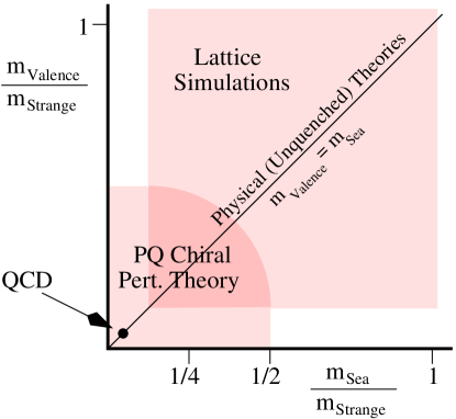
Figure 2.4: Domains for QCD and PQQCD in quark mass space. Full QCD is represented by the point on the diagonal. $\chi$PT “lives” on the diagonal. Partial quenching opens up the parameter space to the 2-dimensional gray region that has a large overlap with the region where PQ$\chi$PT is applicable. The low-energy parameters for PQ$\chi$PT (which are the same as for $\chi$PT) can be determined from this overlap with improved precision. Figure from Ref. [34] courtesy Ruth Van de Water.

For example, since the valence and ghost quarks have equal masses, the contribution of valence quarks in disconnected quark loop diagrams is eliminated by the ghost quarks. The effects of disconnected loop diagrams are solely due to sea quarks and the physics of the sea sector can be explored by varying the sea quark masses. Furthermore, in the limit where the masses of the sea quarks become equal to those of the valence and ghost quarks, one recovers QCD.

In processes that involve electroweak gauge fields, the “theory space” of PQQCD is enlarged once more since one can chose arbitrary values for the charges of the ghost and sea quarks, $q_{j}$, $q_{l}$, and $q_{r}$ in Eq. (2.46). For example, if one choses $q_{j}=q_{l}=q_{r}=0$ then photons can only couple to valence quarks. In the case $q_{j}=2/3$, $q_{l}=-1/3$, and $q_{r}=-1/3$ contributions of the valence and ghost sectors cancel and photons can only couple to sea quarks [32].

In QQCD the answer to the question raised above is different. The problem with the quenched approximation is that the Goldstone boson singlet is no longer affected by the $U(1)_{A}$ anomaly as in QCD. In other words, the QQCD equivalent of the $\eta^{\prime}$ that is heavy in QCD remains light and must be included in the Q$\chi$PT Lagrangian. This requires the addition of new operators and hence new low-energy constants. In general, the low-energy constants appearing in the Q$\chi$PT Lagrangian are unrelated to those in $\chi$PT and extrapolated quenched lattice data is unrelated to QCD. Although there is some empirical evidence that the difference between QQCD and QCD for some observables is small at large quark masses both theories deviate considerable in the low quark mass region. In fact, several examples show that the behavior of meson loops near the chiral limit is frequently misrepresented in Q$\chi$PT [35, 13, 2, 5]. In the following chapters, we find this is additionally true for a number of meson and baryon hadronic properties.

Chapter 3 Chiral $1/M^{2}$ corrections to $B^{(*)}\rightarrow D^{(*)}$ at Zero Recoil in Q$\chi$PT

In this chapter, we study the semileptonic $B^{(*)}\to D^{(*)}$ decays in the limit that the heavy quark masses are infinite. We calculate the lowest order chiral corrections, which are of ${\mathcal{O}}(1/M^{2})$, from the breaking of heavy quark symmetry at the zero recoil point in Q$\chi$PT. These results will aid in the extrapolation of quenched lattice calculations from the light quark masses used on the lattice down to the physical ones.

3.1 Introduction

The Cabibbo-Kobayashi-Maskawa (CKM) matrix describes the flavor mixing among the quarks; its elements are fundamental input parameters for the standard model. Their precise knowledge is not only crucial to determine the standard model but also to shed light on the origin of $CP$ violation. The matrix element that parametrizes the amount of mixing between the $b$ and $c$ quarks, $V_{cb}$, can be extracted from the exclusive semileptonic $B$ meson decays $B\to Dl\nu$ and $B\to D^{*}l\nu$, where $l=e,\mu$. Heavy quark effective theory (HQET) (for a recent review, see [36]), which is exact in the limit of infinite masses $M$ for the heavy quarks, predicts the width of the process $B\to D^{*}l\nu$ as

$$\frac{d\Gamma}{d{\omega}}(B\to D^{*})=\frac{G_{F}^{2}|V_{cb}|^{2}}{48\pi^{3}}{\mathcal{K}}({\omega}){\mathcal{F}}_{B\to D^{*}}({\omega})^{2},$$ (3.1)

where ${\omega}=v\cdot v^{\prime}$ is the scalar product of the 4-velocities $v$ and $v^{\prime}$ of the $B$ and $D^{*}$ mesons, respectively. ${\mathcal{K}}({\omega})$ is a known kinematical factor and ${\mathcal{F}}({\omega})$ is a form factor whose value at the kinematical point ${\omega}=1$ is ${\mathcal{F}}(1)=1$ in the $M\to\infty$ limit. There are, however, perturbative and nonperturbative corrections to ${\mathcal{F}}(1)$,

$${\mathcal{F}}_{B\to D^{*}}(1)=\eta_{A}+{\delta}_{1/M^{2}}+\dots,$$ (3.2)

where the parameter $\eta_{A}\approx 0.96$ is a QCD radiative correction known to two-loop order [37] and ${\delta}_{1/M^{2}}$ are non-perturbative corrections of ${\mathcal{O}}(1/M^{2})$ to the infinite mass limit of HQET. Note that, according to Luke’s theorem [38], there are no ${\mathcal{O}}(1/M)$ corrections at zero-recoil. One chooses the zero-recoil point because, for ${\omega}=1$, ${\mathcal{F}}_{B\to D^{*}}$ can be expressed in terms of a single form factor $h_{A_{1}}$ given by

$$\frac{\langle D^{*}(v,{\epsilon}^{\prime})|\bar{c}\gamma^{\mu}\gamma_{5}b|B(v)\rangle}{\sqrt{m_{B}m_{D^{*}}}}=-2ih_{A_{1}}(1){\epsilon}^{\prime*\mu}.$$ (3.3)

This is in contrast with the general case ${\omega}>1$ for which ${\mathcal{F}}_{B\to D^{*}}({\omega})$ is a linear combination of several different form factors of $B\to D^{*}l\nu$ mediated by vector and axial vector currents.

Several experiments, most recently by CLEO [39], have determined the product $[{\mathcal{F}}_{B\to D^{*}}(1)|V_{cb}|]^{2}$ by measuring $d\Gamma_{B\to D^{*}}/d{\omega}$ and extrapolating it to the zero-recoil point. The mixing parameter $|V_{cb}|$ can then be extracted once the value ${\mathcal{F}}_{B\to D^{*}}(1)$ that encodes the strong interaction physics has been evaluated. The uncertainty in $|V_{cb}|$ is therefore determined by the experimental errors and by theoretical uncertainties in the determination of ${\mathcal{F}}_{B\to D^{*}}(1)$. Presently, the theoretical uncertainties dominate.

A model-independent way of calculating ${\mathcal{F}}(1)$ is provided by numerical lattice QCD simulations. Recently, such calculations have been performed [40, 41, 42, 43] for the decays $B\to D^{(*)}l\nu$ using QQCD. Several systematic uncertainties, such as from statistics and lattice space dependence, contribute to the error of these calculations. Another contribution to the uncertainties comes from the chiral extrapolation of the light quark mass. This extrapolation can be done by matching QQCD to Q$\chi$PT and calculating the non-analytic corrections ${\delta}_{1/M^{2}}$ in Eq. (3.2) in Q$\chi$PT. The formally dominant contributions to these corrections come from the hyperfine mass splitting between the heavy pseudoscalar and vector mesons that stems from the inclusion of heavy quark symmetry breaking operators of ${\mathcal{O}}(1/M)$ in the Lagrangian.

In QCD, the corrections due to $D$ meson hyperfine splitting have been calculated in $\chi$PT by Randall and Wise [44]. A more complete treatment, involving additional corrections due to $B$ meson hyperfine splitting, ${\mathcal{O}}(1/M)$ axial vector coupling corrections, and ${\mathcal{O}}(1/M)$ corrections to the current, has been given in [45]. Recently, the $D$ meson hyperfine splitting corrections have also been determined in PQ$\chi$PT [46] for PQQCD.

In this chapter, we calculate the ${\mathcal{O}}(1/M^{2})$ corrections in Eq. (3.2) due to $D$ and $B$ meson hyperfine splitting in Q$\chi$PT. These corrections are—upon expanding in powers of the hyperfine splitting ${\Delta}$—of order ${\Lambda_{\text{QCD}}}^{3n/2}/(M^{n}m_{q}^{n/2})$ for $n\geq 2$ and formally larger than those coming from the inclusion of ${\mathcal{O}}(1/M)$ heavy quark symmetry breaking operators in the Lagrangian and current which are suppressed by powers of ${\Lambda_{\text{QCD}}}/M$. This argument is similar to the one that applies to $\chi$PT [36]. Our Q$\chi$PT calculation can be used to extrapolate lattice results [42] that use the quenched approximation down to the physical light quark masses. So far, this extrapolation has been based upon the $\chi$PT calculation [44]. Using Q$\chi$PT should therefore give a better estimate of the uncertainties related to the chiral extrapolation.

A central role in the lattice calculation of $B\to D^{*}$ [42, 43] is played by the double ratios of matrix elements

$${\mathcal{R}}_{+}=\frac{\langle D|\bar{c}{\gamma}^{0}b|B\rangle\langle B|\bar{b}{\gamma}^{0}c|D\rangle}{\langle D|\bar{c}{\gamma}^{0}c|D\rangle\langle B|\bar{b}{\gamma}^{0}b|B\rangle},$$ (3.4)

$${\mathcal{R}}_{1}=\frac{\langle D^{*}|\bar{c}{\gamma}^{0}b|B^{*}\rangle\langle B^{*}|\bar{b}{\gamma}^{0}c|D^{*}\rangle}{\langle D^{*}|\bar{c}{\gamma}^{0}c|D^{*}\rangle\langle B^{*}|\bar{b}{\gamma}^{0}b|B^{*}\rangle},$$ (3.5)

and

$${\mathcal{R}}_{A_{1}}=\frac{\langle D^{*}|\bar{c}{\gamma}^{j}{\gamma}_{5}b|B\rangle\langle B^{*}|\bar{b}{\gamma}^{j}{\gamma}_{5}c|D\rangle}{\langle D^{*}|\bar{c}{\gamma}^{j}{\gamma}_{5}c|D\rangle\langle B^{*}|\bar{b}{\gamma}^{j}{\gamma}_{5}b|B\rangle}.$$ (3.6)

In these ratios, statistical fluctuations are highly correlated and cancel to a large degree. The ${\mathcal{O}}(1/M^{2})$ correction to the double ratios can therefore be calculated fairly accurately and used to derive the ${\mathcal{O}}(1/M^{2})$ correction to the matrix elements themselves. For this reason, we also calculate ${\mathcal{O}}(1/M^{2})$ corrections to the decay $B^{*}\rightarrow D^{*}$ in addition to the experimentally accessible decays $B\rightarrow D$ and $B\rightarrow D^{*}$, and thus the corrections to ${\mathcal{R}}_{+}$, ${\mathcal{R}}_{1}$, and ${\mathcal{R}}_{A_{1}}$.

3.2 Quenched Heavy Meson Chiral Perturbation Theory

The $D$ mesons with quantum numbers of $c\bar{Q}$ can be written as a six-component vector

$$D=(D_{u},D_{d},D_{s},D_{\tilde{u}},D_{\tilde{d}},D_{\tilde{s}}).$$ (3.7)

Heavy quark symmetry is provided by combining creation and annihilation operators for the pseudoscalar and vector mesons, $D$ and $D^{*}$, respectively, together into the field $H^{D}$:

$$H^{D} = \frac{1+v\hskip-5.0pt/}{2}(D\hskip-6.49994pt/^{*}+i\gamma_{5}D),$$ (3.8)

$$\bar{H}^{D}=\gamma^{0}H^{D\dagger}\gamma^{0} = ({D\hskip-6.49994pt/^{*}}^{\dagger}+i\gamma_{5}D^{\dagger})\frac{1+v\hskip-5.0pt/}{2},$$ (3.9)

where $v$ denotes the velocity of a heavy meson. In HQET the momentum of a heavy quark is only changed by a small residual momentum of ${\mathcal{O}}(\Lambda_{\text{QCD}})$. Hence, $v$ is not changed and $H$ is usually denoted by an index $v$ which we have dropped here to unclutter the formalism. In the heavy quark limit, the dynamics of the heavy mesons are described by the Lagrangian [47, 48]

$${\cal L}_{D}=-i\,\text{tr}[\bar{H}_{a}^{D}v_{\mu}(\partial^{\mu}{\delta}_{ab}+iV_{ba}^{\mu})H_{b}^{D}]+g\,\text{tr}(\bar{H}_{a}^{D}H_{b}^{D}\gamma_{\nu}\gamma_{5}A_{ba}^{\nu})+{\gamma}\,\text{tr}(\bar{H}_{a}^{D}H_{a}^{D}\gamma_{\mu}\gamma_{5})\,\text{str}A^{\mu}$$ (3.10)

where the traces tr() are over Dirac indices and supertraces str() over the flavor indices are implicit. The additional coupling term involving $\Phi_{0}\sim\text{str}A^{\mu}$ is a feature of Q$\chi$PT and not present in $\chi$PT. The light-meson fields are

$$A_{\mu}=\frac{i}{2}(\xi^{\dagger}\partial_{\mu}\xi-\xi\partial_{\mu}\xi^{\dagger})=-\frac{1}{f}\partial_{\mu}\Phi+{\mathcal{O}}(\Phi^{3})$$ (3.11)

and

$$V_{\mu}=\frac{i}{2}(\xi^{\dagger}\partial_{\mu}\xi+\xi\partial_{\mu}\xi^{\dagger})=\frac{i}{2f^{2}}[\Phi,\partial_{\mu}\Phi]+{\mathcal{O}}(\Phi^{4}).$$ (3.12)

Expanding the Lagrangian ${\cal L}_{D}$ to lowest order in the meson fields leads to the (derivative) couplings $DD^{*}\partial\phi$ and $D^{*}D^{*}\partial\phi$ whose coupling constants are equal as a consequence of heavy quark spin symmetry. At leading order in the $1/M$ expansion, the $DD\partial\phi$ coupling vanishes by parity.

An analogous formalism applies to the fields $B$ and $B^{*}$ which are combined into $H^{B}$. Note that the axial coupling $g$ is the same for $H^{D}$ and $H^{B}$ mesons at this order in the $1/M$ expansion as dictated by heavy quark flavor symmetry.

We do not include terms of order $m_{q}\sim\sqrt{m_{\pi}}$ in the Lagrangian as explicit chiral symmetry breaking effects are suppressed compared to the leading corrections. The presence of these terms is implied by the nonzero meson masses $m_{qq}$.

3.3 Matrix Elements of $\bar{B}^{(*)}\rightarrow D^{(*)}l\bar{\nu}$

The non-zero hadronic matrix elements for $B^{(*)}\rightarrow D^{(*)}$ can be defined in terms of the 16 independent form factors $h_{\pm}$, $h_{V}$, $h_{A_{1,2,3}}$, and $h_{1\dots 10}$ as [49, 36]

$$\frac{\langle D(v^{\prime})|\bar{c}\gamma^{\mu}b|B(v)\rangle}{\sqrt{m_{B}m_{D}}}=h_{+}({\omega})(v+v^{\prime})^{\mu}+h_{-}({\omega})(v-v^{\prime})^{\mu},$$ (3.13)

$$\frac{\langle D^{*}(v^{\prime},{\epsilon}^{\prime})|\bar{c}\gamma^{\mu}b|B(v)\rangle}{\sqrt{m_{B}m_{D^{*}}}}=-h_{V}({\omega})\varepsilon^{\mu\nu{\alpha}{\beta}}{\epsilon}^{\prime*}_{\nu}v^{\prime}_{\alpha}v_{\beta},$$ (3.14)

$$\frac{\langle D^{*}(v^{\prime},{\epsilon}^{\prime})|\bar{c}\gamma^{\mu}\gamma_{5}b|B(v)\rangle}{\sqrt{m_{B}m_{D^{*}}}}=-ih_{A_{1}}({\omega})({\omega}+1){\epsilon}^{\prime*\mu}+ih_{A_{2}}({\omega})(v\cdot{\epsilon}^{\prime*})v^{\mu}+ih_{A_{3}}({\omega})(v\cdot{\epsilon}^{\prime*})v^{\prime\mu},$$ (3.15)

$$\frac{\langle D^{*}(v^{\prime},{\epsilon}^{\prime})|\bar{c}\gamma^{\mu}b|B^{*}(v,{\epsilon})\rangle}{\sqrt{m_{B^{*}}m_{D^{*}}}} = -({\epsilon}^{\prime*}\cdot{\epsilon})[h_{1}({\omega})(v+v^{\prime})^{\mu}+h_{2}({\omega})(v-v^{\prime})^{\mu}]+h_{3}({\omega})({\epsilon}^{\prime*}\cdot v){\epsilon}^{\mu}$$

$$+h_{4}({\omega})({\epsilon}\cdot v^{\prime}){\epsilon}^{\prime*\mu}-({\epsilon}\cdot v^{\prime})({\epsilon}^{\prime*}\cdot v)[h_{5}({\omega})v^{\mu}+h_{6}({\omega})v^{\prime\mu}],$$

and

$$\frac{\langle D^{*}(v^{\prime},{\epsilon}^{\prime})|\bar{c}\gamma^{\mu}\gamma_{5}b|B^{*}(v,{\epsilon})\rangle}{\sqrt{m_{B^{*}}m_{D^{*}}}} = i\varepsilon^{\mu{\alpha}{\kappa}{\delta}}\left\{{\epsilon}^{*}_{\kappa}{\epsilon}_{\delta}\left[h_{7}({\omega})(v+v^{\prime})^{\mu}+h_{8}({\omega})(v-v^{\prime})^{\mu}\right]\right.$$

$$\left.\phantom{dadasd}+v^{\prime{\alpha}}v^{\beta}\left[h_{9}({\omega})({\epsilon}^{\prime*}\cdot v){\epsilon}^{\mu}+h_{10}({\omega})({\epsilon}\cdot v^{\prime}){\epsilon}^{\prime*\mu}\right]\right\}.$$

Here, ${\omega}=v\cdot v^{\prime}$ and $v$ (${\epsilon}$) and $v^{\prime}$ (${\epsilon}^{\prime}$) are the velocities (polarization vectors) of the initial state $B^{(*)}$ meson and final state $D^{(*)}$ meson, respectively. Note that we will not explicitly calculate matrix elements of $B^{*}\to D$ as these can be easily related to the $B\to D^{*}$ calculation by a Hermitian conjugation of the matrix elements and an interchange of the $c$ and $b$ quarks, i.e., $B^{(*)}\leftrightarrow D^{(*)}$.

In the heavy quark limit the matrix elements in Eqs. (3.13)–(3.3) are reproduced by the operator

$$\bar{c}\gamma^{\mu}(1-\gamma_{5})b\rightarrow-\xi(\omega)\text{tr}[\bar{H}^{D}_{v^{\prime}}\gamma^{\mu}(1-\gamma_{5})H^{B}_{v}].$$ (3.18)

Here, $\xi({\omega})$ is the universal Isgur-Wise function [50, 51] with the normalization $\xi(1)=1$. To lowest order in the heavy quark expansion one finds

$$h_{+}({\omega})=h_{V}({\omega})=h_{A_{1}}({\omega})=h_{A_{3}}({\omega})=h_{1}({\omega})=h_{3}({\omega})=h_{4}({\omega})=h_{7}({\omega})=\xi({\omega})$$ (3.19)

and the remaining 8 form factors vanish.

The discussion of the $\bar{B}^{(*)}\rightarrow D^{(*)}l\bar{\nu}$ matrix elements is similar for different flavors of the light quark $q$ content of the $B^{(*)}$ and $D^{(*)}$ mesons; it applies equally to $q=u$, $d$, or $s$ as the theory splits into three similar copies of a one-flavor theory. In the limit of light quark $SU(3)_{V}$ flavor symmetry the matrix elements (and in particular the Isgur-Wise function) are therefore independent of the light quark flavor. However, in nature the masses of the $u$, $d$, and $s$ quarks are different and $SU(3)_{V}$ is not an exact symmetry. Therefore our results will include terms that depend upon $m_{q}$ via the meson masses $m_{qq}$ defined in Eq. (2.38).

3.4 $1/M^{2}$ Corrections

The lowest order heavy quark symmetry violating operator that can be included in the Lagrangian ${\mathcal{L}}_{D}$ in Eq. (3.10) is the dimension-three operator $({\lambda}_{D_{2}}/M_{D})\text{tr}\left(\bar{H_{a}}^{D}\sigma^{\mu\nu}H_{a}^{D}\sigma_{\mu\nu}\right)$. It violates heavy-quark spin and flavor symmetries and comes from the QCD magnetic moment operator $\bar{c}\sigma^{\mu\nu}G_{\mu\nu}^{A}T^{A}c$, where $G_{\mu\nu}^{A}$ is the gluon field strength tensor and $T^{A}$ with $A=1,\dots,8$ are the eight color $SU(3)$ generators. This operator gives rise to a mass difference between the $D$ and $D^{*}$ mesons of

$${\Delta}_{D}=m_{D^{*}}-m_{D}=-8\frac{{\lambda}_{D_{2}}}{\bar{M}_{D}}.$$ (3.20)

This effect can be taken into account by modifying the $D$ and $D^{*}$ propagators which become

$$\frac{i{\delta}_{ab}}{2(v\cdot k+3{\Delta}_{D}/4+i{\epsilon})}\quad\text{and}\quad\frac{-i{\delta}_{ab}(g_{\mu\nu}-v_{\mu}v_{\nu})}{2(v\cdot k-{\Delta}_{D}/4+i{\epsilon})},$$ (3.21)

respectively, so that in the rest frame, where $v=(1,0,0,0)$, an on-shell $D$ has residual energy of $-3{\Delta}_{D}/4$ and an on-shell $D^{*}$ has residual energy of ${\Delta}_{D}/4$. A similar effect due to the inclusion of a QCD magnetic moment operator for the $b$ quark applies to the $B^{(*)}$ mesons.

There are no corrections to the matrix elements for the semileptonic decays $B^{(*)}\rightarrow D^{(*)}e\nu$ of ${\mathcal{O}}(1/M)$ at zero-recoil according to Luke’s theorem [38]. The leading corrections enter at ${\mathcal{O}}(1/M^{2})$. In addition to tree-level contributions from the insertion of ${\mathcal{O}}(1/M^{2})$ suppressed operators into the heavy quark Lagrangian or the current there are one-loop contributions from wave function renormalization and vertex correction. These one-loop diagrams have a non-analytic dependence on the meson mass $m_{qq}$ and depend on the subtraction point $\mu$. This dependence on $\mu$ is canceled by the tree-level contribution of the ${\mathcal{O}}(1/M^{2})$ operators.

Because of the absence of disconnected quark loops in QQCD, which manifests itself as a cancellation between intermediate pseudo Goldstone bosons and pseudo Goldstone fermions in loops in Q$\chi$PT, the only loop diagrams that survive are those that contain a hairpin interaction or a ${\gamma}$ coupling [see Eq. (3.10)].

The wave function renormalization contributions for the pseudoscalar and vector meson, $Z_{D/B}$ and $Z^{*}_{D/B}$, respectively, come from the one-loop diagrams shown in Fig. 3.1 and have been calculated in [35, 47, 48].

Figure 3.1: Graphs contributing to wavefunction renormalization for heavy (a) pseudoscalar and (b) vector mesons. A thin (thick) line denotes a heavy pseudoscalar (vector) meson, a dashed line denotes the $\Phi_{0}$, while a dashed-crossed line denotes the insertion of a hairpin. A full (empty) vertex denotes a $g$ (${\gamma}$) coupling.

Including the ${\alpha}$ coupling we find, for these diagrams,

$$Z = 1+\frac{ig^{2}\mu_{0}^{2}}{f^{2}}H_{1}({\Delta})-\frac{ig^{2}{\alpha}}{f^{2}}H_{2}({\Delta})+\frac{6i{\gamma}g}{f^{2}}F_{1}({\Delta})$$ (3.22)

and

$$Z^{*} = 1+\frac{ig^{2}\mu_{0}^{2}}{3f^{2}}H_{1}(-{\Delta})-\frac{ig^{2}{\alpha}}{3f^{2}}H_{2}(-{\Delta})+\frac{2i{\gamma}g}{f^{2}}F_{1}(-{\Delta})$$ (3.23)

$$+\frac{2ig^{2}\mu_{0}^{2}}{3f^{2}}H_{1}(0)-\frac{2ig^{2}{\alpha}}{3f^{2}}H_{2}(0)+\frac{4i{\gamma}g}{f^{2}}F_{1}(0).$$

The functions $H_{1}$, $H_{2}$, and $F_{1}$ come from loop integrals and are given in Appendix B. Note that in the heavy quark limit where ${\Delta}=0$ one recovers $Z=Z^{*}$, as required by heavy quark symmetry.

The vertex corrections come from one-loop diagrams. The non-vanishing contributions are shown in Fig. 3.2.

Figure 3.2: Q$\chi$PT graphs which contribute to the vertex correction of the form factors (a) $h_{+}(1)$, (b) $h_{A_{1}}(1)$, and (c) $h_{1}(1)$. A full (empty) square denotes the insertion of the operator $\bar{c}{\gamma}^{\mu}{\gamma}_{5}b$ ($\bar{c}{\gamma}^{\mu}b$).

Combining the wave function renormalization and vertex corrections and including a local counterterm to cancel the dependence on the renormalization scale $\mu$, we find the following corrections for the form factors:

$${\delta}h_{+}(1) = X_{+}(\mu)+\frac{Z_{B}-1}{2}+\frac{Z_{D}-1}{2}$$ (3.24)

$$-\frac{ig^{2}}{f^{2}}\left[\mu_{0}^{2}\,H_{5}({\Delta}_{B},{\Delta}_{D})-{\alpha}\,H_{8}({\Delta}_{B},{\Delta}_{D})\right]-\frac{6ig{\gamma}}{f^{2}}G_{5}({\Delta}_{B},{\Delta}_{D})$$

$$\rightarrow X_{+}(\mu)+\frac{1}{(4\pi f)^{2}}\left(\frac{g^{2}\mu_{0}^{2}}{3m^{2}}-\left[\frac{g^{2}{\alpha}}{3}-2g{\gamma}\right]\log\frac{m^{2}}{\mu^{2}}\right)({\Delta}_{B}-{\Delta}_{D})^{2}$$

$$+{\mathcal{O}}(\{{\Delta}_{B},{\Delta}_{D}\}^{3}),$$

$${\delta}h_{A_{1}}(1) = X_{A_{1}}(\mu)+\frac{Z_{B}-1}{2}+\frac{Z_{D}^{*}-1}{2}$$

$$-\frac{ig^{2}}{3f^{2}}\left[\mu_{0}^{2}\,H_{5}({\Delta}_{B},-{\Delta}_{D})-{\alpha}\,H_{8}({\Delta}_{B},-{\Delta}_{D})\right]-\frac{2ig{\gamma}}{f^{2}}G_{5}({\Delta}_{B},-{\Delta}_{D})$$

$$-\frac{2ig^{2}}{3f^{2}}\left[\mu_{0}^{2}\,H_{5}({\Delta}_{B},0)-{\alpha}\,H_{8}({\Delta}_{B},0)\right]-\frac{4ig{\gamma}}{f^{2}}G_{5}({\Delta}_{B},0)$$

$$\rightarrow X_{A_{1}}(\mu)+\frac{1}{(4\pi f)^{2}}\left(\frac{g^{2}\mu_{0}^{2}}{9m^{2}}-\left[\frac{g^{2}{\alpha}}{9}-\frac{2g{\gamma}}{3}\right]\log\frac{m^{2}}{\mu^{2}}\right)\left(3{\Delta}_{B}^{2}+{\Delta}_{D}^{2}+2{\Delta}_{B}{\Delta}_{D}\right)$$ (3.25)

$$+{\mathcal{O}}(\{{\Delta}_{B},{\Delta}_{D}\}^{3}),$$

and

$${\delta}h_{1}(1) = X_{1}(\mu)+\frac{Z_{B}^{*}-1}{2}+\frac{Z_{D}^{*}-1}{2}$$ (3.26)

$$-\frac{ig^{2}}{3f^{2}}\left[\mu_{0}^{2}\,H_{5}(-{\Delta}_{B},-{\Delta}_{D})-{\alpha}\,H_{8}(-{\Delta}_{B},-{\Delta}_{D})\right]-\frac{2ig{\gamma}}{f^{2}}G_{5}(-{\Delta}_{B},-{\Delta}_{D})$$

$$-\frac{2ig^{2}}{3f^{2}}\left[\mu_{0}^{2}\,H_{5}(0,0)-{\alpha}\,H_{8}(0,0)\right]-\frac{4ig{\gamma}}{f^{2}}G_{5}(0,0)$$

$$\rightarrow X_{1}(\mu)+\frac{1}{(4\pi f)^{2}}\left(\frac{g^{2}\mu_{0}^{2}}{9m^{2}}-\left[\frac{g^{2}{\alpha}}{9}-\frac{2g{\gamma}}{3}\right]\log\frac{m^{2}}{\mu^{2}}\right)\left({\Delta}_{B}-{\Delta}_{D}\right)^{2}$$

$$+{\mathcal{O}}(\{{\Delta}_{B},{\Delta}_{D}\}^{3}),$$

which are defined by $h_{+}(1)=1+{\delta}h_{+}(1)$ and analog expressions for ${\delta}h_{A_{1}}(1)$ and ${\delta}h_{1}(1)$. The functions $H_{5}$, $H_{8}$, and $G_{5}$ come from loop-integrals that are listed in Appendix B and we have defined $m=m_{qq}$. The insertions of tree-level ${\mathcal{O}}(1/M^{2})$ operators are represented by the functions $X_{+}(\mu)$, $X_{A_{1}}(\mu)$, and $X_{1}(\mu)$ which are independent of $m$ and exactly cancel the $\mu$ dependence of the logarithm. These functions can be extracted from lattice simulations by measuring the zero-recoil form factors for a varying mass of the light quark.

Experimentally, ${\Delta}_{D}\approx 142\,\text{MeV}$ and ${\Delta}_{B}\approx 46\,\text{MeV}$ so that the ratios ${\Delta}_{D}/m$ and ${\Delta}_{B}/m$, which enter the form factor corrections through the function $R({\Delta}/m)$ (defined in Appendix B), are ${\mathcal{O}}(1)$. On the lattice, however, one can vary all quark masses. Expanding first in powers of ${\Delta}$ and then taking the chiral limit $m\to 0$ one finds the formal limits given in Eqs. (3.24)–(3.26) where we have only kept the pieces non-analytic in $m$. This demonstrates that the terms linear in ${\Delta}_{D}$ and ${\Delta}_{B}$, although present in wave function renormalization and vertex corrections, cancel as required by Luke’s theorem [38]. The leading order corrections are ${\mathcal{O}}(\{{\Delta}_{B},{\Delta}_{D}\}^{2})$.

As a consistency check one can restore heavy quark flavor symmetry by taking ${\Delta}_{B}={\Delta}_{D}$. Since the ${\mathcal{O}}(1/M^{2})$ corrections to $h_{+}(1)$ and $h_{1}(1)$ are proportional to $({\Delta}_{B}-{\Delta}_{D})^{2}$ they disappear as they should since the charge associated with the operators $\bar{c}{\gamma}_{\mu}c$ and $\bar{b}{\gamma}_{\mu}b$ is conserved. This argument does not apply for the $B\to D^{*}$ transition matrix element in the limit ${\Delta}_{B}={\Delta}_{D}$ since there is no conserved axial charge associated with the operators $\bar{c}{\gamma}_{\mu}{\gamma}_{5}c$ and $\bar{b}{\gamma}_{\mu}{\gamma}_{5}b$.

In the chiral limit, the term proportional to $\mu_{0}^{2}$ has a $1/m^{2}$ singularity and dominates over the terms proportional to ${\alpha}$ and ${\gamma}$ that are only logarithmically divergent. This is analogous to a term of the form $(m_{qq}^{2}-m_{jj}^{2})/m_{qq}^{2}$ found by Savage [46] for PQ$\chi$PT (here, $m_{qq}$ and $m_{jj}$ are valence and sea quark masses, respectively). In the limit $m_{jj}\to m_{qq}$ this term, however, vanishes as PQ$\chi$PT goes to $\chi$PT where the dominant term is $\log m_{qq}$. In Q$\chi$PT, on the other hand, the $1/m_{qq}^{2}$ pole persists, revealing the sickness of QQCD where the hairpin interactions give a completely different chiral behavior than in QCD.

The size of $\mu_{0}$ can be estimated from the $\eta$-$\eta^{\prime}$ mass splitting [18], large $N_{C}$ arguments [52, 53] ($N_{C}$ being the number of colors), or lattice calculations. These estimates imply $\mu_{0}\approx 500-900\,\text{MeV}$; for the purpose of dimensional analysis we use $\mu_{0}\sim{\mathcal{O}}({\Lambda_{\text{QCD}}})$. Taking $g\sim{\mathcal{O}}(1)$ we therefore find that ${\delta}h_{+}$, ${\delta}h_{A_{1}}$, and ${\delta}h_{1}$ are of order ${\Delta}^{n}/m^{n}\sim{\Lambda_{\text{QCD}}}^{3n/2}/(M^{n}m_{q}^{n/2})$ for $n\geq 2$ and thus larger than tree-level heavy quark symmetry breaking operators that are suppressed by ${\Lambda_{\text{QCD}}}/M$.

To show the dependence of the zero-recoil form factors on the mass of the light spectator quark it is necessary to know the numerical values of the parameters $\mu_{0}$, $g$, ${\alpha}$, and ${\gamma}$. In determining reasonable values for these couplings we follow the discussion by Sharpe and Zhang [48]. Assuming that $g$ is similar to the $\chi$PT value we use $g^{2}=0.4$. The hairpin coupling ${\alpha}$ is proportional to $1/N_{C}$, and thus assumed to be small; we use two values, ${\alpha}=0$ and ${\alpha}=0.7$. The coupling ${\gamma}$ is known to be suppressed by $1/N_{C}$ compared to $g$, the sign is undetermined. We take $-g\leq{\gamma}\leq g$ (see [48] and references therein).

With these parameters, the dependence of $h_{+}(1)$ and $h_{A_{1}}(1)$ on the mass of the light spectator quark $m_{q}$ is show in Figs. 3.3 and 3.4, respectively.

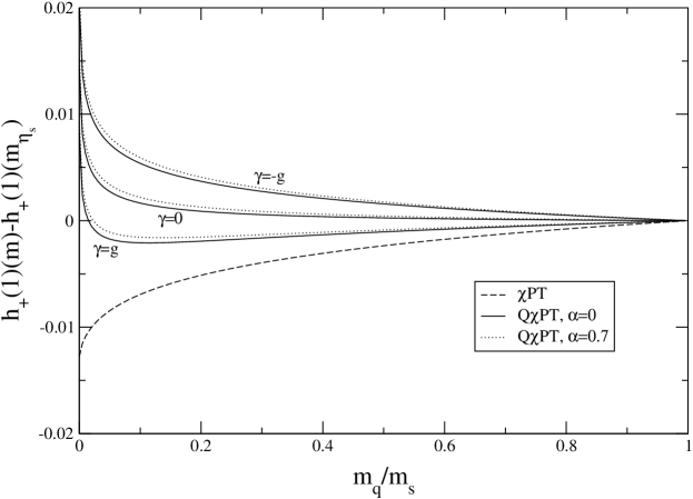
Figure 3.3: Dependence of $h_{+}(1)$ on the mass $m_{q}$ of the light spectator quark in Q$\chi$PT. For comparison, the $\chi$PT result from [44] is also shown (dashed line). The result has been normalized to unity for $m_{q}=m_{s}$. We have chosen $\mu_{0}=700\,\text{MeV}$ and $g^{2}=0.4$.

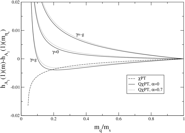
Figure 3.4: Dependence of $h_{A_{1}}(1)$ on the mass of the light spectator quark in Q$\chi$PT. The dashed line denotes the $\chi$PT result [44]. The numerical values for the parameters are those used in Fig. 3.3.

The graphs are plotted against $m_{q}$ in units of the strange quark mass $m_{s}$ with $m_{q}/m_{s}=m^{2}/m_{\eta_{s}}^{2}$ where $m_{\eta_{s}}^{2}=2m_{K}^{2}$. The behavior of $h_{+}(1)$ in Q$\chi$PT is dominated at small $m$ by the $1/m^{2}$ pole that is non-existent in $\chi$PT. Lattice calculations of $h_{+}(1)$ [41] show a small downward trend for decreasing $m_{q}$ down to the chiral limit that is similar to the downward trend seen from the $\chi$PT calculation (dashed line). The same behavior (down to $m_{q}\approx 0.1m_{s}$) can also be seen for Q$\chi$PT for a certain choice of parameters (e.g., ${\gamma}$ positive). The case of $h_{A_{1}}(1)$ is different as there is a pole at $m={\Delta}_{D}$ which is close to the physical pion mass. Here, both $D^{*}$ and $\pi$ can be on-shell and the decay $B\to D^{*}\pi$ becomes kinematically allowed. Lattice calculations of $h_{A_{1}}(1)$ [42] for $m_{q}=(0.6\dots 1)m_{s}$ show a small downward trend for decreasing $m_{q}$ similar to the downward trend seen from the $\chi$PT calculation (dashed line in Fig. 3.4). A similar trend down to $m_{q}\approx 0.2m_{s}$ can also be seen in the Q$\chi$PT calculation for a relatively large positive value of ${\gamma}$.

Although the downward trend in the lattice data for the two cases seems significant as the statistical errors are highly correlated, the uncertainty is still relatively high (typically $\pm 0.01$) and the existing lattice data can be accommodated by a wide range of values for the parameters in the Q$\chi$PT Lagrangian.

As can be seen in the figures, the variation of the quenched result is primarily due to the parameter ${\gamma}$ as the sensitivity of the result to the value of ${\alpha}$ is very small. We have also checked how the result depends on the parameter $g$ in the reasonable range $0.1<g^{2}<0.5$ and found that the change from the value $g^{2}=0.4$ is at most 25% for $g^{2}=0.5$, still well within the statistical errors of the lattice data.

Finally, we calculate the double ratios defined in Eqs. (3.4)–(3.6) using the results in Eqs. (3.24)–(3.26). We find

$${\mathcal{R}}_{+}=1+2{\delta}h_{+}(1),$$ (3.27)

$${\mathcal{R}}_{1}=1+2{\delta}h_{1}(1),$$ (3.28)

and

$${\mathcal{R}}_{A_{1}} = 1+\tilde{X}_{A_{1}}(\mu)$$ (3.29)

$$-\frac{ig^{2}}{3f^{2}}\left\{\mu_{0}^{2}\left[H_{5}({\Delta}_{B},-{\Delta}_{D})+H_{5}({\Delta}_{D},-{\Delta}_{B})-H_{5}({\Delta}_{D},-{\Delta}_{D})-H_{5}({\Delta}_{B},-{\Delta}_{B})\right]\right.$$

$$\left.\phantom{ggggg}-{\alpha}\left[H_{8}({\Delta}_{B},-{\Delta}_{D})+H_{8}({\Delta}_{D},-{\Delta}_{B})-H_{8}({\Delta}_{D},-{\Delta}_{D})-H_{8}({\Delta}_{B},-{\Delta}_{B})\right]\right\}$$

$$-\frac{2ig{\gamma}}{f^{2}}\left[G_{5}({\Delta}_{B},-{\Delta}_{D})+G_{5}({\Delta}_{D},-{\Delta}_{B})-G_{5}({\Delta}_{D},-{\Delta}_{D})-G_{5}({\Delta}_{B},-{\Delta}_{B})\right]$$

$$\rightarrow 1+\tilde{X}_{A_{1}}(\mu)-\frac{1}{(4\pi f)^{2}}\left(\frac{2g^{2}\mu_{0}^{2}}{9m^{2}}-\left[\frac{2g^{2}{\alpha}}{9}-\frac{4g{\gamma}}{3}\right]\log\frac{m^{2}}{\mu^{2}}\right)\left({\Delta}_{B}-{\Delta}_{D}\right)^{2}$$

$$+{\mathcal{O}}(\{{\Delta}_{B},{\Delta}_{D}\}^{3}),$$

where $\tilde{X}_{A_{1}}(\mu)$ is the counterterm associated with ${\mathcal{R}}_{A_{1}}$.

3.5 Conclusions

Knowledge of the $B^{(*)}\to D^{(*)}$ form factors at the zero-recoil point is crucial to extract the value of $V_{cb}$ from experiment. In the limit that the heavy quarks are infinitely heavy, HQET predicts that the form factors $h_{+}$, $h_{A_{1}}$, and $h_{1}$ are equal, $h_{+}(1)=h_{A_{1}}(1)=h_{1}(1)=\xi(1)$. The formally dominant correction due to breaking of heavy quark symmetry comes from the inclusion of a ${\mathcal{O}}(1/M)$ dimension-three operator in the Lagrangian that leads to hyperfine-splitting between the heavy pseudoscalar and vector mesons. These leading order corrections are ${\mathcal{O}}(\{{\Delta}_{B},{\Delta}_{D}\}^{2}$ as required by Luke’s theorem.

Recent lattice simulations using the quenched approximation of QCD have made a big step forward in determining these zero-recoil form factors. Presently, however, the simulations use light quark masses that are much heavier than the physical ones and therefore rely on a chiral extrapolation down to the physical quark masses. In this chapter we have calculated the dominant corrections to the form factors $h_{+}$, $h_{A_{1}}$, and $h_{1}$ in Q$\chi$PT and determined the non-analytic dependence on the light quark masses via the light meson masses $m_{qq}$. Using these results, instead of the $\chi$PT calculation, to extrapolate the QQCD lattice measurements of these form factors down to the physical pion mass should give a more reliable estimate of the errors associated with the chiral extrapolation. We have also calculated the corrections to certain double ratios that are used in lattice QCD calculations of the decay $B\to D^{*}$.

Chapter 4 HM$\chi$PT in a Finite Volume

In this chapter, we study finite volume effects in heavy quark systems in the framework of heavy meson chiral perturbation theory (HM$\chi$PT) for QCD, QQCD, and PQQCD. A novel feature of this investigation is the role played by the scales ${\Delta}$ and ${\delta}_{s}$, where ${\Delta}$ is the mass difference between the heavy-light vector and pseudoscalar mesons of the same quark content, and ${\delta}_{s}$ is the difference of the masses of the $u$ and $d$, and the mass of the $s$ quark that is due to light flavour $SU(3)$ breaking. The primary conclusion of this chapter is that finite volume effects arising from the propagation of Goldstone mesons in the effective theory can be altered by the presence of these scales. Since ${\Delta}$ varies significantly with the heavy quark mass, these volume effects can be amplified in both heavy and light quark mass extrapolations.

As an explicit example, we present results for $B$ parameters of neutral $B$ meson mixing matrix elements and heavy-light decay constants to one-loop order in finite volume HM$\chi$PT for full, quenched, and $N_{f}=2+1$ partially quenched QCD. Our calculation shows that for high-precision determinations of the phenomenologically interesting $SU(3)$ breaking ratios, finite volume effects are significant in QQCD and not negligible in PQQCD, although they are generally small in QCD.

4.1 Introduction

Numerical calculations of hadronic properties using LQCD have provided significant inputs to particle physics phenomenology. In particular, the joint effort between experiment and theory to investigate the unitarity triangle in the CKM matrix from $B$ meson decays and mixing has made impressive progress [54], in which LQCD has played an important role. Nevertheless, current lattice calculations are still subject to various systematic errors. In this chapter, we address finite volume effects which arise in lattice calculations for heavy-light meson systems from the light degrees of freedom. Our framework is HM$\chi$PT with first order $1/M$ and chiral corrections. We assume the mass hierarchy

$$m_{QQ^{\prime}}\ll\Lambda_{\chi}\ll M,$$ (4.1)

where $m_{QQ^{\prime}}$ is the mass of any Goldstone meson given in Eqs. (2.20) and (2.38) and $M$ is the mass of the heavy-light meson. Under this assumption, we discard corrections of the size

$$\frac{m_{QQ^{\prime}}}{M}.$$ (4.2)

Concerning the finite volume, we work with the condition that

$$m_{QQ^{\prime}}L\gg 1,$$ (4.3)

where $L$ is the spatial extent of the cubic box. Therefore, given that $f_{\pi}L/\sqrt{2}$ ($f_{\pi}\approx 132\text{ MeV}$) will be close to one in lattice simulations in the near future, one can still neglect the chiral symmetry restoration effects resulting from the Goldstone zero momentum modes [55, 56] when Eq. (4.3) is satisfied.

The main task of this work is to study the volume effects due to the presence of the scales

$${\Delta}=M_{P^{\ast}}-M_{P},$$ (4.4)

and

$$\delta_{s}=M_{P_{s}}-M_{P},$$ (4.5)

where $P^{\ast}$ and $P$ are the heavy-light vector and pseudoscalar mesons containing a $u$ or $d$ anti-quark,and $P_{s}$ is the heavy-light pseudoscalar meson with an $s$ anti-quark. The scale ${\Delta}$ appears due to the breaking of heavy quark spin symmetry that is of ${\mathcal{O}}(1/M)$ and $\delta_{s}$ comes from light flavour $SU(3)$ breaking in the heavy-light meson masses. Under the assumption of Eq. (4.1), ${\Delta}$ is independent of the light quark mass, and $\delta_{s}$ does not contain any $1/M$ corrections, at the order we are working.

In the real world, both ${\Delta}$ and $\delta_{s}$ are not very different from the pion mass. In fact [1], $M_{B_{s}}-M_{B}=91\text{ MeV}$, $M_{D_{s}}-M_{D}=104\text{ MeV}$, $M_{B^{\ast}}-M_{B}=46\text{ MeV}$, and $M_{D^{\ast}}-M_{D}=142\text{ MeV}$. In current lattice simulations, these mass splittings vary between 0 and $\sim 150$ MeV. Therefore it is important to include them in the investigation of finite volume effects. Equation (4.3) implies that the Compton wavelength of the Goldstone meson is small compared to the size of the box. Therefore finite volume effects mainly result from the propagation of the Goldstone mesons to the boundary. However, as shown in Section 4.3, ${\Delta}$ and $\delta_{s}$ can, in a non-trivial way, alter these effects. In particular, since ${\Delta}$ varies with the heavy quark mass, finite volume effects can be significantly amplified in heavy quark mass extrapolations.

This chapter is organized as follows. In Section 4.2 we summarize the ingredients of HM$\chi$PT relevant to this work. We mainly expand the treatment in Section 3.2 to the partially quenched case. Section 4.3 is devoted to the discussion of HM$\chi$PT in finite volume, emphasising the role played by $\delta_{s}$ and ${\Delta}$. We then present an explicit calculation of neutral $B$ meson mixing and heavy-light decay constants in Section 4.4 and discuss the phenomenological impact that finite volume effects can have. We conclude in Section 4.5. Some mathematical formulae and results are summarized in Appendix C.

4.2 Partially Quenched Heavy Meson Chiral Perturbation Theory

The chiral Lagrangian for the Goldstone mesons in the three theories QCD, QQCD, and PQQCD has been discussed in detail in Chapter 2 and we will not repeat it here. The inclusion of the heavy-light mesons into the quenched version of HM$\chi$PT has been discussed in Section 3.2. Here we will expand this discussion and also include the cases of QCD and PQQCD.

HM$\chi$PT was first proposed in Refs. [57, 58, 59], with the generalization to quenched and partially quenched theories given in Refs. [47, 48]. The $1/M$ and chiral corrections were studied by Boyd and Grinstein [60] in QCD and by Booth [35] in QQCD. The spinor field appearing in this effective theory is

$$H^{(Q)}_{a}=\frac{1+v\hskip-5.0pt/}{2}\left(P^{\ast(Q)}_{a,\mu}\gamma^{\mu}-P^{(Q)}_{a}\gamma_{5}\right),$$ (4.6)

where $P^{(Q)}_{a}$ and $P^{\ast(Q)}_{a,\mu}$ annihilate pseudoscalar and vector mesons containing a heavy quark $Q$ and a light anti-quark of flavour $a$.

The HM$\chi$PT Lagrangian, to lowest order in the chiral and $1/M$ expansion, for $D$ mesons containing a heavy quark $c$ and a light anti-quark of flavour $a$ is then given in Eq. (3.10). The Lagrangian for a heavy $B$ meson containing a $b$ quark is analogous. In QCD, the term proportional to ${\gamma}$ is non-existent as the $\eta^{\prime}$ is integrated out. We do not formally distinguish the coupling $g$ in the three theories with the understanding that the numerical values are different. The HM$\chi$PT Lagrangian for mesons containing a heavy anti-quark $\bar{Q}$ and a light quark of flavour $a$ is obtained by applying the charge conjugation operation to the Lagrangian in Eq. (3.10) [61]. At this order, the propagators for $P^{(Q)}_{a}$ and $P^{\ast(Q)}_{a}$ mesons are

$$\frac{i}{2(v\cdot k+i\epsilon)}\quad\text{and}\quad\frac{-i(g_{\mu\nu}-v_{\mu}v_{\nu})}{2(v\cdot k+i\epsilon)},$$ (4.7)

respectively.

The effects of chiral and heavy quark symmetry breaking have been systematically studied in full [60] and quenched [35] HM$\chi$PT. Amongst them, the only relevant feature necessary for the purpose of this work, i.e., the investigation of finite volume effects, are the shifts to the masses of the heavy-light mesons. These shifts are from the heavy quark spin breaking term

$$\frac{\lambda_{2}}{M}{\text{tr}_{D}}\left(\bar{H}^{(Q)}_{a}\sigma_{\mu\nu}H^{(Q)}_{a}\sigma^{\mu\nu}\right),$$ (4.8)

and the chiral symmetry breaking terms

$$\lambda_{1}B_{0}\text{tr}_{D}\left(\bar{H}^{(Q)}_{a}\left[\xi m_{Q}\xi+\xi^{\dagger}M_{Q}\xi^{\dagger}\right]_{ab}H^{(Q)}_{b}\right)+\lambda_{1}^{\prime}B_{0}\text{tr}_{D}\left(\bar{H}^{(Q)}_{a}H^{(Q)}_{a}\right)\left[\xi m_{Q}\xi+\xi^{\dagger}m_{Q}\xi^{\dagger}\right]_{bb}.$$ (4.9)

We choose to work with the effective theory in which the heavy-light pseudoscalar mesons that contain a heavy quark and a $u$ or $d$ valence anti-quark are massless. Notice that the term proportional to $\lambda^{\prime}_{1}$ in Eq. (4.9) causes a universal shift to all the heavy-light meson masses. This means that the masses appearing in the propagators of heavy vector mesons and any meson containing an $s$ anti-quark (valence or ghost) are shifted as follows:

$$\frac{-i(g_{\mu\nu}-v_{\mu}v_{\nu})}{2(v\cdot k-{\Delta}+i\epsilon)},\quad\frac{i}{2(v\cdot k-\delta_{s}+i\epsilon)},\quad\text{and}\quad\frac{-i(g_{\mu\nu}-v_{\mu}v_{\nu})}{2(v\cdot k-{\Delta}-\delta_{s}+i\epsilon)},$$ (4.10)

for $P^{\ast}$, $P_{s}$, and $P^{\ast}_{s}$, respectively. The mass shifts can be written in terms of the couplings in Eqs. (4.8) and (4.9), ${\Delta}=-8\lambda_{2}/M$ , and

$$\delta_{s}=2\lambda_{1}B_{0}(m_{s}-m_{u}).$$ (4.11)

In PQQCD, there are two additional mass shifts because the sea quarks have different masses from the valence and ghost quarks:

$$\tilde{\delta}_{s}=M_{\tilde{P}_{s}}-M_{\tilde{P}}=2\lambda_{1}B_{0}(m_{r}-m_{j}),$$ (4.12)

and

$$\delta_{\mathrm{sea}}=M_{\tilde{P}}-M_{P}=2\lambda_{1}B_{0}(m_{j}-m_{u}).$$ (4.13)

where $\tilde{P}$ ($\tilde{P}_{s}$) is the heavy-light pseudoscalar meson with a $d$ ($s$) sea anti-quark. The propagators of the heavy mesons containing sea anti-quarks are:

$$\frac{i}{2(v\cdot k-\delta_{\mathrm{sea}}+i\epsilon)},\quad\frac{-i(g_{\mu\nu}-v_{\mu}v_{\nu})}{2(v\cdot k-{\Delta}-\delta_{\mathrm{sea}}+i\epsilon)},$$ (4.14)

$$\frac{i}{2(v\cdot k-\delta_{\mathrm{sea}}-\tilde{\delta}_{s}+i\epsilon)},\quad\text{and}\quad\frac{-i(g_{\mu\nu}-v_{\mu}v_{\nu})}{2(v\cdot k-{\Delta}-\delta_{\mathrm{sea}}-\tilde{\delta}_{s}+i\epsilon)}$$ (4.15)

for $\tilde{P}$, $\tilde{P}^{*}$ (vector meson with a $d$ sea anti-quark), $\tilde{P}_{s}$, and $\tilde{P}^{*}_{s}$ (vector meson with an $s$ sea anti-quark), respectively.

4.3 Finite Volume Effects

In this section, we discuss generic features of finite volume effects in HM$\chi$PT. For clarity, we use the symbol $\Delta$ for one of (${\Delta}$, $\delta_{s}$, $\tilde{\delta}_{s}$, $\delta_{\mathrm{sea}}$) or any sum amongst them.

In the limit where the heavy quark mass goes to infinity and the light quark masses are equal, all the heavy mesons in HM$\chi$PT become on-shell static sources, and there is a velocity superselection rule when the momentum transfer involved in the scattering of the heavy meson system is fixed [62]. For illustration, consider the vertex with coupling $g$ in the Lagrangian in Eq. (3.10). The heavy-light meson $P$ can scatter into $P^{\ast}_{(s)}$ by emitting a Goldstone meson with mass $m_{QQ^{\prime}}$ through this vertex. The momenta of the mesons $P$ and $P^{\ast}_{(s)}$ are $M_{P}v_{\mu}$, and $M_{P^{\ast}_{(s)}}v_{\mu}+k_{\mu}=M_{P}v_{\mu}+k_{\mu}$, where the velocity $v_{\mu}=(1,0,0,0)$ in the rest frame of the heavy mesons, and $k_{\mu}$ is the soft momentum carried by the Goldstone meson. The infinitely heavy $P$ and $P^{\ast}_{(s)}$ mesons do not propagate in space. Therefore, when such a system is in a cubic spatial box, finite volume effects result entirely from the propagation of the Goldstone meson to the boundary with momentum $k\sim m_{QQ^{\prime}}$. In this case the volume effects behave like $\exp{(-m_{QQ^{\prime}}L)}$ multiplied by a polynomial in $1/L$.

The breaking of heavy quark spin and $SU(3)$ light flavour symmetries in HM$\chi$PT can induce a mass difference $M_{P^{\ast}_{(s)}}=M_{P}+\Delta$, which complicates the above picture. In this scenario, the $P^{\ast}_{(s)}$ is still regarded as a static source, but it is off-shell with the virtuality $\Delta$. The period during which the Goldstone meson can propagate to the boundary is limited by the time uncertainty conjugate to this virtuality, i.e.,

$$\delta t\sim\frac{1}{\Delta}.$$ (4.16)

This means that finite volume effects, which arise from the propagation of the Goldstone mesons in such a system, will decrease as $\Delta$ increases. Eq. (4.16) also indicates that the suppression of the volume effects by a non-zero $\Delta$ is controlled by the parameter

$$\frac{m_{QQ^{\prime}}}{\Delta}.$$ (4.17)

To see explicitly how this phenomenon appears in a calculation, we consider a typical sum in one-loop HM$\chi$PT, with a Goldstone propagator and a heavy-light vector meson propagator in the loop, in a cubic box with periodic boundary conditions:

$${\mathcal{J}}(m,\Delta)=-i\frac{1}{L^{3}}\sum_{\vec{k}}\int\frac{dk_{0}}{2\pi}\frac{1}{(k^{2}-m^{2}+i\epsilon)(v\cdot k-\Delta+i\epsilon)},$$ (4.18)

where the spatial momentum $\vec{k}$ is quantized in finite volume as $\vec{k}=(2\pi/L)\vec{i}$, with $\vec{i}$ being a three dimensional integer vector. Using the Poisson summation formula, it is straightforward to show that ${\mathcal{J}}(m,\Delta)=J(m,\Delta)+{J_{\text{FV}}}(m,\Delta)$, where

$$J(m,\Delta)=-i\int\frac{d^{4}k}{(2\pi)^{4}}\frac{1}{(k^{2}-m^{2}+i\epsilon)(v\cdot k-\Delta+i\epsilon)},$$ (4.19)

is the infinite volume limit of ${\mathcal{J}}(m,\Delta)$, and

$${J_{\text{FV}}}(m,\Delta)=\frac{1}{4\pi^{2}}\sum_{\vec{n}\not=\vec{0}}\int_{0}^{\infty}d|\vec{k}|\frac{|\vec{k}|}{{\omega}({\omega}+\Delta)}\frac{\sin(|\vec{k}||\vec{n}|L)}{|\vec{n}|L},$$ (4.20)

with ${\omega}=\sqrt{|\vec{k}|^{2}+m^{2}}$, is the finite volume correction to $J(m,\Delta)$. In the asymptotic limit where $mL\gg 1$ it can be shown that (with $n=|\vec{n}|$)

$${J_{\text{FV}}}(m,\Delta)=\sum_{\vec{n}\not=\vec{0}}\frac{1}{8\pi nL}\exp(-nmL)\,{\mathcal{A}},$$ (4.21)

where

$${\mathcal{A}} = \exp(z^{2})[1-{\text{erf}}(z)]+\frac{1}{nmL}\left[\frac{1}{\sqrt{\pi}}\left(\frac{z}{4}-\frac{z^{3}}{2}\right)+\frac{z^{4}}{2}\exp(z^{2})[1-{\text{erf}}(z)]\right]$$ (4.22)

$$-\frac{1}{(nmL)^{2}}\left[\frac{1}{\sqrt{\pi}}\left(\frac{9z}{64}-\frac{5z^{3}}{32}+\frac{7z^{5}}{16}+\frac{z^{7}}{8}\right)-\left(\frac{z^{6}}{2}+\frac{z^{8}}{8}\right)\exp(z^{2})[1-{\text{erf}}(z)]\right]$$

$$+{\mathcal{O}}\left(\frac{1}{(nmL)^{3}}\right),$$

with

$$z=\frac{\Delta}{m}\sqrt{\frac{nmL}{2}}.$$ (4.23)

The quantity ${\mathcal{A}}$ is the alteration of finite volume effects due to the presence of a non-zero $\Delta$. It multiplies the factor $\exp(-nmL)$, which results from the propagation of the Goldstone meson to the boundary. It is possible to analytically compute the higher order corrections of ${\mathcal{A}}$ in powers of $1/(nmL)$. This way, one can achieve any desired numerical precision. Here it is clear that this alteration of volume effects is controlled by the ratio in Eq. (4.17).

Next, we consider different limits of ${\mathcal{A}}$ at fixed $m$ and $L$. When $\Delta=0$, clearly ${\mathcal{A}}=1$. If $\Delta$ is very small compared to $m$, such that $z\ll 1$, ${\mathcal{A}}$ is dominated by the $[1/(mL)]^{0}$ term, i.e., ${\mathcal{A}}\approx\exp(z^{2})[1-{\text{erf}}(z)]$. Since ${\text{erf}}(z)$ grows much faster than exp($z^{2}$) in this regime, ${\mathcal{A}}$ will decrease as $\Delta$ increases. When $\Delta$ is of ${\mathcal{O}}(m)$ or larger, $z\gg 1$, and one can perform an asymptotic expansion of the error function. It can be shown that in this situation, ${\mathcal{A}}\sim 1/z$. That is, ${\mathcal{A}}$ also decreases as $\Delta$ increases. We have also numerically checked that this is true when $z\approx 1$. This means that the asymptotic formula in Eq. (4.21) reproduces the physical picture outlined in the beginning of this section for any $\Delta$. To demonstrate how fast the asymptotic form in Eq. (4.22) converges to Eq. (4.20), we define

$$d{J_{\text{FV}}}(m,\Delta)=\frac{{J_{\text{FV}}}^{\mathrm{num}}(m,\Delta)-{J_{\text{FV}}}^{\mathrm{asymp}}(m,\Delta)}{{J_{\text{FV}}}^{\mathrm{num}}(m,\Delta)},$$ (4.24)

where ${J_{\text{FV}}}^{\mathrm{num}}$ is the function ${J_{\text{FV}}}$ evaluated numerically [Eq. (4.20)], and ${J_{\text{FV}}}^{\mathrm{asymp}}$ is the asymptotic form in Eq. (4.22). In Fig. 4.1,

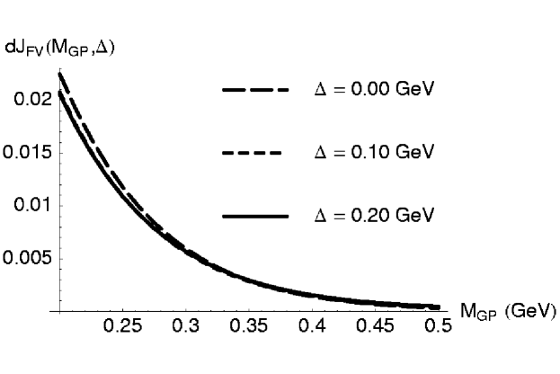
Figure 4.1: $d{J_{\text{FV}}}(m,\Delta)$ plotted against $m$ for three different $\Delta$. This function indicates the deviation (in percent) of the asymptotic form of ${J_{\text{FV}}}$ from the definition in Eq. (4.20). In this plot, $L=$2.5 fm and $m=0.197$ GeV corresponds to $mL=2.5$ whereas $m=0.32$ GeV corresponds to $mL=4$. The curve for $\Delta=0.1$ GeV is hidden by that for $\Delta=0.2$ GeV.

we plot $d{J_{\text{FV}}}$ as a function of $m$ with three choices of $\Delta$. It is clear from this plot that ${J_{\text{FV}}}$ is approximated well (to $\leq 3\%$) by the asymptotic form when $mL\geq 2.5$. We use the asymptotic forms for integrals of this type throughout this work. Also, in this paper we only include the terms with $|\vec{n}|=1$,$\sqrt{2}$, $\sqrt{3}$, $\sqrt{4}$, and $\sqrt{5}$ in the Poisson summation formula. We have confirmed that truncating the sum at $|\vec{n}|=\sqrt{5}$ is a very good approximation (to $\sim 3\%$) when $mL\geq 2.5$. The function ${J_{\text{FV}}}(m,\Delta)$ is plotted against $m$ in Fig. 4.2,

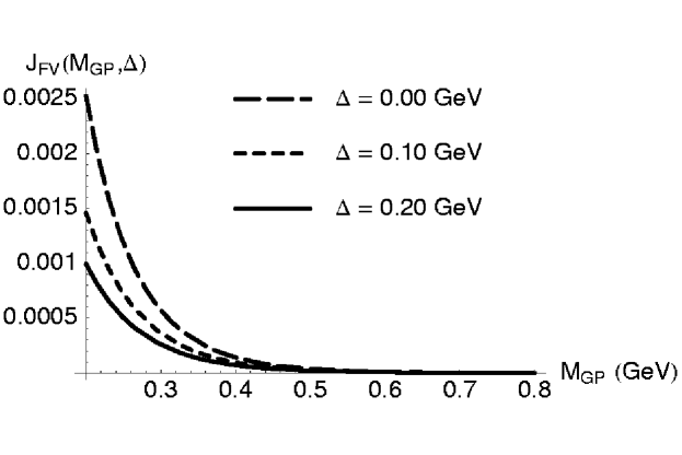
Figure 4.2: ${J_{\text{FV}}}(m,\Delta)$ plotted as a function of $m$, for three different $\Delta$. Again, $L=$2.5 fm.

with $L=2.5$ fm and three choices of $\Delta$. It is clear from this plot that $\Delta$ can significantly alter the finite volume effects in ${\mathcal{J}}(m,\Delta)$.

Another typical sum that appears in one-loop HM$\chi$PT in finite volume is

$${\mathcal{K}}(m,\Delta)=-\frac{i}{L^{3}}\sum_{\vec{k}}\int\frac{dk_{0}}{2\pi}\frac{1}{(k^{2}-m^{2}+i\epsilon)(v\cdot k-\Delta+i\epsilon)^{2}}.$$ (4.25)

It is straightforward to show that ${\mathcal{K}}(m,\Delta)=K(m,\Delta)+{K_{\text{FV}}}(m,\Delta)$, where

$$K(m,\Delta)=\frac{\partial}{\partial\Delta}J(m,\Delta)$$ (4.26)

is the infinite volume limit of ${\mathcal{K}}(m,\Delta)$ and

$${K_{\text{FV}}}(m,\Delta)=\frac{\partial}{\partial\Delta}{J_{\text{FV}}}(m,\Delta)$$ (4.27)

is the finite volume correction to $K(m,\Delta)$. The function ${K_{\text{FV}}}(m,\Delta)$ is plotted against $m$ in Fig. 4.3,

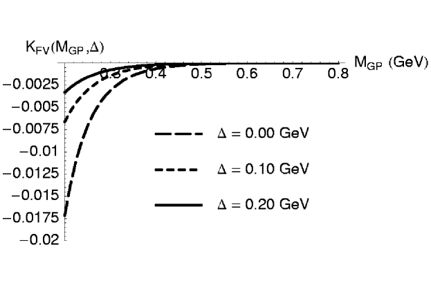
Figure 4.3: ${K_{\text{FV}}}(m,\Delta)$ plotted as a function of $m$ for three different $\Delta$. Again, $L=2.5$ fm.

with $L=2.5$ fm and three choices of $\Delta$. As expected, $|{K_{\text{FV}}}(m,\Delta)|$ also decreases when $\Delta$ increases at fixed $m$ and $L$.

4.4 Neutral $B$ Mixing and Heavy-Light Decay Constants

The study of neutral $B$ meson mixing allows the extraction of the magnitude of the CKM matrix element $V_{td}$, and hence the determination of one of the sides of the unitarity triangle. The frequency of the $B_{d}{-}\bar{B}_{d}$ oscillations, which is given by the mass difference, $\Delta m_{d}$, in this mixing system has been well measured by various experimental collaborations [54]. It is also calculable in the standard model via an operator product expansion in which the top quark and $W$ boson are integrated out. Resumming the next-to-leading order (NLO) short-distance QCD effects, one obtains

$$\Delta m_{d}=\frac{G_{F}}{8\pi^{2}}M^{2}_{W}|V_{td}V^{\ast}_{tb}|^{2}\eta_{B}S_{0}(x_{t})C_{B}(\mu)\frac{|\langle\bar{B}_{d}|{\mathcal{O}}^{\Delta B=2}_{d}(\mu)|B_{d}\rangle|}{2M_{B}},$$ (4.28)

where $\mu$ is the renormalisation scale, $x_{t}=m^{2}_{t}/M^{2}_{W}$, and $S_{0}(x_{t})\approx 0.784x_{t}^{0.76}$ (to better than $1\%$) is the relevant Inami-Lim function [63]. The coefficients $\eta_{B}=0.55$ and $C_{B}(\mu)$ are from short-distance QCD effects [64, 65]. The matrix element of the four-quark operator

$${\mathcal{O}}^{\Delta B=2}_{d}=[\bar{b}\gamma^{\mu}(1-\gamma_{5})d][\bar{b}\gamma_{\mu}(1-\gamma_{5})d]$$ (4.29)

between $B_{d}$ and $\bar{B}_{d}$ states contains all the long-distance QCD effects in Eq. (4.28), and has to be calculated non-perturbatively. Since $|V_{tb}|=1$ to good accuracy and $\Delta m_{d}$ has been well measured, a high-precision calculation of $\langle\bar{B}_{d}|{\mathcal{O}}^{\Delta B=2}_{d}(\mu)|B_{d}\rangle$ enables a clean determination of $|V_{td}|$.

The frequency of the rapid $B_{s}{-}\bar{B}_{s}$ oscillations can be precisely measured at the Tevatron and LHC [54]. Therefore an alternative approach is to consider the ratio

$$\frac{\Delta m_{s}}{\Delta m_{d}}=\left|\frac{V_{ts}}{V_{td}}\right|^{2}\frac{M_{B_{d}}}{M_{B_{s}}}\left|\frac{\langle\bar{B}_{s}|{\mathcal{O}}^{\Delta B=2}_{s}|B_{s}\rangle}{\langle\bar{B}_{d}|{\mathcal{O}}^{\Delta B=2}_{d}|B_{d}\rangle}\right|,$$ (4.30)

in which many theoretical uncertainties cancel. Here $\Delta m_{s}$ is the mass difference in the $B_{s}{-}\bar{B}_{s}$ system and ${\mathcal{O}}^{\Delta B=2}_{s}=[\bar{b}\gamma^{\mu}(1-\gamma_{5})s][\bar{b}\gamma_{\mu}(1-\gamma_{5})s]$. The unitarity of the CKM matrix implies $|V_{ts}|\approx|V_{cb}|$ to a few percent, and $|V_{cb}|$ can be precisely extracted by analysing semileptonic $B$ decays [54]. Therefore a clean measurement of $\Delta m_{s}/\Delta m_{d}$ will yield an accurate determination of $|V_{td}|$.

The matrix elements in Eq. (4.30) are conventionally parameterized as

$$\langle\bar{B}_{q}|{\mathcal{O}}^{\Delta S=2}_{q}|B_{q}\rangle=\frac{8}{3}M^{2}_{B_{q}}f^{2}_{B_{q}}B_{B_{q}}(\mu),$$ (4.31)

where the parameter $B_{B_{q}}$ measures the deviation from the vacuum-saturation approximation of the matrix element, and $q=d$ or $s$. The decay constant $f_{B_{q}}$ is defined by

$$\langle 0|\bar{b}\gamma_{\mu}\gamma_{5}q|B_{q}(\vec{p})\rangle=ip_{\mu}f_{B_{q}}.$$ (4.32)

LQCD provides a reliable tool for calculating these non-perturbative QCD quantities from first principles. Since $\Delta m_{s}/\Delta m_{d}$ will be measured to very good accuracy, it is important to have clean theoretical calculations for [the $SU(3)$ breaking ratios of] the matrix elements, decay constants and $B$ parameters involved. Current lattice calculations have to be combined with effective theories in order to obtain these matrix elements at the physical quark masses. This procedure can introduce significant systematic errors and dominate the uncertainties in the $SU(3)$ breaking ratio[75, 76]

$$\xi=\frac{f_{B_{s}}\sqrt{B_{B_{s}}}}{f_{B}\sqrt{B_{B}}},$$ (4.33)

which is the key theoretical input for future high-precision determination of $|V_{td}|$ via the study of neutral $B$ mixing. However, the use of effective theory also offers a framework for studying finite volume effects in lattice calculations [18, 77, 78, 26, 79, 80, 81, 82, 83, 84, 85, 86, 87, 88, 89]. We will demonstrate in this section that finite volume effects might turn out to exceed the current quoted systematic errors for quantities such as $\xi$.

4.4.1 One-Loop Calculation in a Finite Volume

Here, we discuss one-loop calculations for the $B$ parameters and heavy-light decay constants mentioned above in finite volume HM$\chi$PT including the appropriate mass shifts to the first non-trivial order of the chiral and $1/M$ expansion. The inclusion of other first-order corrections in these quantities is straightforward. It simply introduces additional low-energy constants (LECs) which account for short-distance physics and do not give rise to finite volume effects at this order, so we will not discuss this issue here. We have performed the calculation for QCD, QQCD and PQQCD with the mass shifts given in Eqs. (4.10)–(4.15).

For the purpose of this work, the axial current $\bar{b}\gamma_{\mu}\gamma_{5}q_{a}$ is

$$A_{\mu}=\frac{\kappa}{2}\text{tr}_{\mathrm{D}}\left[\gamma_{\mu}\gamma_{5}H^{(Q)}_{b}\xi^{\dagger b}_{a}\right],$$ (4.34)

and the four-quark operator ${\mathcal{O}}^{\Delta P_{a}=2}$ (when $P_{a}=B_{d,s}$, ${\mathcal{O}}^{\Delta P_{a}=2}$ becomes ${\mathcal{O}}^{\Delta B=2}_{d,s}$) is

$$O^{aa}=4\beta\left[\left(\xi P^{\ast(Q)\dagger}_{\mu}\right)^{a}\left(\xi P^{\ast(\bar{Q})\mu}\right)^{a}+\left(\xi P^{(Q)\dagger}\right)^{a}\left(\xi P^{(\bar{Q})}\right)^{a}\right]$$ (4.35)

in HM$\chi$PT [61], where $\kappa$ and $\beta$ are the low-energy constants which have to be determined from experiments or lattice calculations. Notice that the index $a$ in Eq. (4.35) is not summed over. Again, the inclusion of the chiral and $1/M_{P}$ corrections in these operators simply introduces additional LECs and we do not investigate this aspect here. We assume that $\kappa$ and $\beta$ are the same in QCD, QQCD, and PQQCD. Also, $A_{\mu}$ and $O^{aa}$ can couple to the $\eta^{\prime}$ in QQCD, but the couplings are $1/N_{c}$ suppressed [48], and we neglect them.

The diagrams contributing to $f_{P_{(s)}}$ and $B_{P_{(s)}}$ are presented in Figs. 4.4–4.6.

Figure 4.4: Wave-function renormalization diagrams for heavy-light mesons

Figure 4.5: Diagrams contributing to the one-loop calculation of decay constants. The thin (thick) solid lines are the heavy-light pseudoscalar (vector) mesons. The dashed lines are Goldstone mesons, and the crosses are the “double poles” which appear in (P)Q$\chi$PT. The open squares are the operators defined in Eq. (4.34) and the dots are vertices from the HM$\chi$PT Lagrangian.

Figure 4.6: Diagrams contributing to the one-loop calculation of the $B$ parameters. The open circles are the operators defined in Eq. (4.35).

Note that only diagrams with an intermediate heavy meson depend on the heavy meson mass shifts.

Although this is the first one-loop calculation for these decay constants and $B$ parameters in finite volume, some results in the infinite volume limit already exist in the literature: $f_{P_{(s)}}$ have been calculated at the lowest order in QCD [61], QQCD [48, 47], and PQQCD [48], and up to first-order corrections in the chiral and $1/M$ expansions in QCD [60] and QQCD [35]. The $B$ parameters have been calculated only at lowest order [61, 48]. Our results, as presented in Appendix C.2, agree with all these previous calculations in the appropriate limits.

4.4.2 Phenomenological Impact

We have used the one-loop results in Appendix C.2 to investigate the impact of finite volume effects on $\xi$. In this work, we only intend to estimate the possible size of errors in this quantity, and will leave the actual comparison with lattice data to a future publication. Following the usual procedure in lattice calculations for $\xi$, we study two $SU(3)$ breaking ratios

$$\xi_{f}=\frac{f_{B_{s}}}{f_{B}}$$ (4.36)

and

$$\xi_{B}=\frac{B_{B_{s}}}{B_{B}},$$ (4.37)

in terms of which, $\xi=\xi_{f}\sqrt{\xi_{B}}$. Furthermore, we define $(\xi_{f})_{\mathrm{FV}}$ and $(\xi_{B})_{\mathrm{FV}}$ to be the contributions from finite volume effects, i.e., those from the volume-dependent part in the one-loop results presented in Subsection 4.4.1. To be more precise, we use the formulae collected in Appendix C.2 to calculate the volume corrections with respect to the lowest-order values of $f_{B_{s}}$ ($B_{B_{s}}$) and $f_{B}$ ($B_{B}$), then take the difference between the results as an estimate of $(\xi_{f})_{\mathrm{FV}}$ [$(\xi_{B})_{\mathrm{FV}}$]. Since these $SU(3)$ ratios are not very different from unity (at most $\sim 20\%$), this is a reasonable estimate of these effects.

Traditionally, many quenched lattice simulations of $B_{B_{(s)}}$ and $f_{B_{(s)}}$ were performed using $L\sim 1.6$ fm. Therefore we present our estimate for finite volume effects in QQCD with this box size. For comparison, we adopt the same volume for QCD. As for PQQCD, we work with $L=2.5$ fm where most current high-precision simulations are carried out [90]. Throughout this subsection, we ensure that the condition $M_{\pi}L\geq 2.5$ holds in all the plots presented here.

We first discuss the procedure in QCD and QQCD. When studying the light quark mass dependence of $(\xi_{f})_{\mathrm{FV}}$ and $(\xi_{B})_{\mathrm{FV}}$, we follow a strategy similar to that in Ref. [75]. That is, we use the Gell-Mann-Okubo formulae to express $M_{K}$ and $M_{\eta}$ in terms of $M_{\pi}$ and $m_{ss}$:

$$M^{2}_{K}=\frac{m^{2}_{ss}+M^{2}_{\pi}}{2}\quad\text{and}\quad M^{2}_{\eta}=\frac{2m^{2}_{ss}+M^{2}_{\pi}}{3}.$$ (4.38)

We investigate the situation where a lattice calculation is performed at the physical strange quark mass $(m_{s})_{\mathrm{phys}}$, but the up and down quark mass $m_{u}=m_{d}$ is varied. By using $(M_{K})_{\mathrm{phys}}=0.498$ GeV and $(M_{\pi})_{\mathrm{phys}}=0.135$ GeV [1], we fix $(m_{ss})_{\mathrm{phys}}=2B_{0}(m_{s})_{\mathrm{phys}}=0.691$ GeV as an input parameter in our analysis. Notice that $(m_{ss})_{\mathrm{phys}}$ is not the mass of a “physical” meson, and the subscript just means this mass is estimated by using physical kaon and pion masses. To the same order, we can adopt Eq. (4.11) to write $\delta_{s}=\lambda_{1}\left(m^{2}_{ss}-M^{2}_{\pi}\right)$, and use $(m_{ss})_{\mathrm{phys}}$, $(M_{\pi})_{\mathrm{phys}}$ and physical $M_{B_{s}}-M_{B}=0.091$ GeV [1] to determine

$$\lambda_{1}=0.1982\mbox{ GeV}^{-1}.$$ (4.39)

This determines how $\delta_{s}$ varies with $M_{\pi}$. We have also tried to use vanishing pion mass and $M_{D_{s}}-M_{D}=0.104$ GeV [1] to fix $(m_{ss})_{\mathrm{phys}}$ and $\lambda_{1}$, and the results presented in this subsection are not sensitive to this variation from the values quoted above.

The results for $(\xi_{f})_{\mathrm{FV}}$ and $(\xi_{B})_{\mathrm{FV}}$ for QCD and QQCD from this analysis are presented in Figs. 4.7–4.10

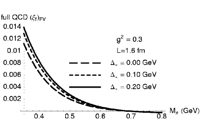
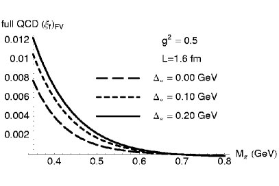
Figure 4.7: $(\xi_{f})_{\mathrm{FV}}$ in full QCD plotted against $M_{\pi}$ with $L=1.6$ fm. The pion mass $M_{\pi}=0.35$ GeV corresponds to $M_{\pi}L=2.8$, and $M_{\pi}=0.5$ GeV corresponds to $M_{\pi}L=4$.

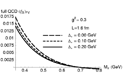
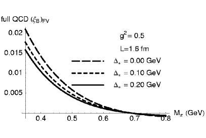
Figure 4.8: $(\xi_{B})_{\mathrm{FV}}$ in full QCD plotted against $M_{\pi}$ with $L=1.6$ fm.

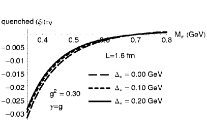
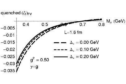
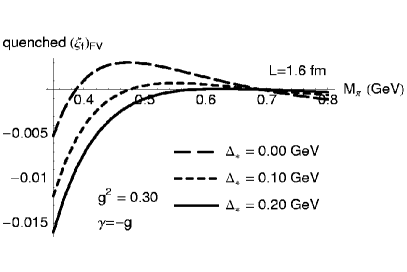
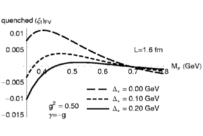
Figure 4.9: $(\xi_{f})_{\mathrm{FV}}$ in QQCD plotted against $M_{\pi}$, with $L=1.6$ fm and different couplings $g$ and $\gamma$. We set $\alpha=0$ and $M_{0}=700$ MeV.

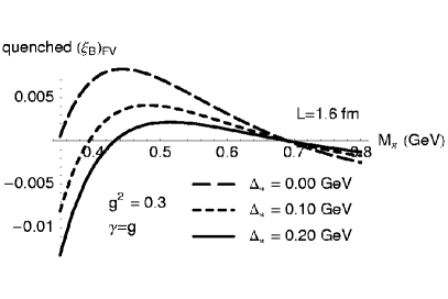
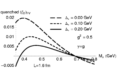
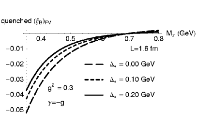
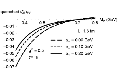
Figure 4.10: $(\xi_{B})_{\mathrm{FV}}$ in QQCD plotted against $M_{\pi}$, with $L=1.6$ fm, $\alpha=0$ and $M_{0}=700$ MeV, and different couplings.

with two different values for the coupling $g$ (and also $\gamma$ in QQCD). Here we stress again that the influence on finite volume effects from the presence of $\Delta$ and $\delta_{s}$ depends on the size of these couplings, which are not well determined. Inspired by the recent CLEO measurement of $g$ in the charm system [91, 92], and a recent lattice calculation [93], we vary $g^{2}$ between 0.3 and 0.5. As for the coupling $\gamma$, which is a quenching artifact and has never been determined, we vary its value between $g$ and $-g$. It is clear from these plots that the finite volume effects are generally small in QCD ($\leq 2\%$), but can be significant in QQCD ($\sim 3\%$ to $\sim 7\%$ for $\xi_{B}$) in the range of $M_{\pi}L$ where lattice simulations are normally performed. This is clearly due to the enhanced long-distance effect arising from the “double pole” structure in (P)QQCD, as first pointed out in Ref. [77], and manifests itself in various places, e.g., nucleon-nucleon potentials [94] and $\pi{-}\pi$ scattering [77, 95, 82, 81].

Although it has been well established that infinite volume chiral corrections are smaller in the $B$ parameters than in the decay constants due to the coefficient in front of $g^{2}$ in the one-loop results, it is clear from these plots that finite volume effects are more salient in $\xi_{B}$ than in $\xi_{f}$. All the quenched lattice calculations for $\xi_{B}$ have so far concluded that this quantity is consistent with unity with typically $3\%$ error. However, we find that the volume effects are already at the level of $3{-}4\%$ when $M_{\pi}=0.45$ GeV in a 1.6 fm box where many quenched simulations were carried out. This error depends on both light and heavy quark masses in the simulation, hence is amplified after extrapolating the result to the physical quark masses. Also, the fact that volume effects tend towards different directions in QCD and QQCD when $M_{\pi}$ becomes smaller indicates that quenching errors in these quantities can be larger than those estimated in Ref. [48]. Since finite volume effects have not been included in the analysis of lattice calculations of $\xi_{B}$ hitherto, one should be cautious when using the existing quenched results for this quantity in any phenomenological work.

For the analysis in PQQCD, we assume that both the valence and sea strange quark masses are fixed at that of the physical strange quark. However, we vary the light sea quark mass $m_{j}=m_{l}$. For this purpose, we define $m_{jj}$ to be the mass of the meson composed of two light sea quarks. Therefore,

$$\frac{m^{2}_{jj}}{(m_{ss}^{2})_{\mathrm{phys}}}=\left(\frac{m_{j}}{m_{r}}\right)_{m_{r}\,=\,{\text{physical }}m_{s}}.$$ (4.40)

Also, we can express the mass shifts $\tilde{\delta}_{s}$ and $\delta_{\mathrm{sea}}$ in terms of meson masses, $\tilde{\delta}_{s}=\lambda_{1}\left(m_{ss}^{2}-m_{rr}^{2}\right)$ and $\delta_{\mathrm{sea}}=\lambda_{1}\left(m^{2}_{rr}-M^{2}_{\pi}\right)$ by using Eqs. (4.12) and (4.13) with the same value for $\lambda_{1}$ used in Eq. (4.39).

The results for the PQQCD analysis are presented in Figs. 4.11 and 4.12.

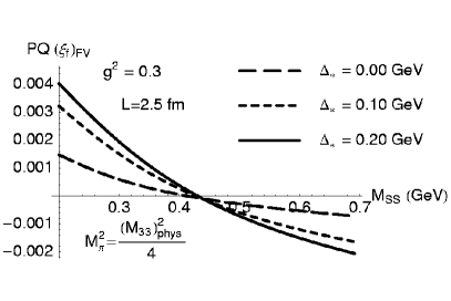
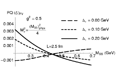
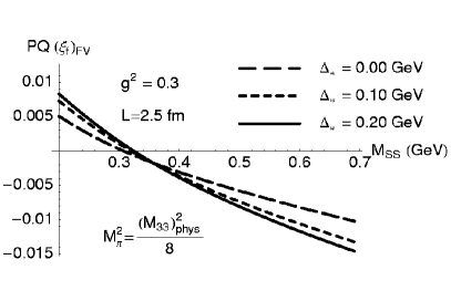
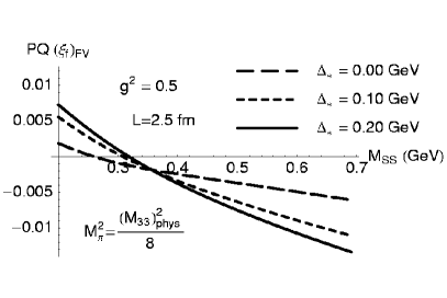
Figure 4.11: $(\xi_{f})_{\mathrm{FV}}$ in PQQCD plotted against $m_{rr}$, with $L=2.5$ fm and two different values for $M_{\pi}$. The pion mass $M^{2}_{\pi}=m^{2}_{ss}/4$ corresponds to $M_{\pi}L=4.4$ and $M^{2}_{\pi}=m^{2}_{ss}/8$ corresponds to $M_{\pi}L=3.1$. The mass $m_{rr}=0.197$ GeV corresponds to $m_{rr}L=2.5$, and $m_{rr}=0.32$ GeV corresponds to $m_{rr}L=4$.

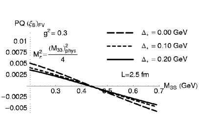
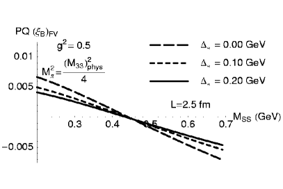
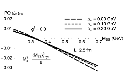
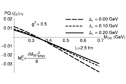
Figure 4.12: $(\xi_{B})_{\mathrm{FV}}$ in PQQCD plotted against $m_{rr}$ with $L=2.5$ fm and two different values for $M_{\pi}$.

The double pole insertions also appear in PQQCD and it is clear from these plots that finite volume effects cannot be neglected if one hopes to determine $\xi$ to the level of a few percent. Especially, in the range of $M_{\pi}$ and $L$ where current and future lattice simulations are performed [90], they can already be at about $4\%$, and the dependence on the heavy meson mass is quite strong. Therefore they can become comparable to the error presented in the latest review [74], $\xi=1.23\pm 0.10$ after quark mass extrapolations.

4.5 Conclusions

We have investigated finite volume effects in heavy quark systems in the framework of HM$\chi$PT. The primary conclusion is that the scales ${\Delta}$ and $\delta_{s}$, which are heavy-light meson mass splittings arising from the breaking of heavy quark spin and light flavour $SU(3)$ symmetries, can significantly reduce the volume effects in diagrams involving heavy meson propagators in the loop. The physical picture of this phenomenon is that some heavy-light mesons are off-shell in the effective theory, as a consequence of the velocity superselection rule, with the virtuality characterized by the mass splittings. The time uncertainty conjugate to this virtuality limits the period during which the Goldstone mesons can propagate to the boundary. Finite volume effects caused by the propagation of the Goldstone mesons naturally affect the light quark mass extrapolation/interpolation in a lattice calculation. On top of this, our work implies that they also influence the heavy quark mass extrapolation/interpolation, since the scale ${\Delta}$ varies significantly with the heavy meson mass. The strength of this influence is process-dependent, determined also by the relative weight between diagrams with and without heavy meson propagators in the loop. The volume effects can be amplified by both heavy and light quark mass extrapolations. Therefore it is important to perform calculations to identify these effects in phenomenologically interesting quantities.

We have presented an explicit calculation in finite volume HM$\chi$PT for the $B$ parameters in neutral $B$ meson mixing and heavy-light decay constants, in QCD, QQCD, and PQQCD. We have used these results to estimate the impact of finite volume effects in the $SU(3)$ ratio $\xi$, which is an important input in determining the magnitude of the CKM matrix element $V_{td}$. Within the parameter space where most quenched lattice calculations have been performed, we find that, although this impact is quite small ($\leq\sim 2\%$) in QCD, it can be significant in QQCD. This is due to the enhanced long-distance effects arising from the double pole structure. This error will be amplified by the quark mass extrapolations and hence can exceed the currently quoted systematic effects. Furthermore, finite volume effects tend towards different directions in QCD and QQCD for decreasing $M_{\pi}$. This means that quenching errors in $\xi$ may be significantly larger than what was estimated before. Therefore one has to be cautious when using the existing quenched lattice QCD results for $\xi$ in phenomenological work. In PQQCD, our results indicate that finite volume effects are typically between $3\%$ and $5\%$ in the data range of future high-precision simulations, and they can be significantly amplified in the procedure of quark mass extrapolations. This means that they are not negligible in future lattice calculations of $\xi$.

Chapter 5 Charge Radii of the Meson and Baryon Octets in Q$\chi$PT and PQ$\chi$PT

In this chapter, we calculate the electric charge radii of the $SU(3)$ pseudoscalar mesons as well as the $SU(3)$ octet baryons in Q$\chi$PT and PQ$\chi$PT. The results are needed for the extrapolation of future lattice calculations of these observables. We also derive expressions for the nucleon and pion charge radii in $SU(2)$ flavor away from the isospin limit.

5.1 Introduction

The study of hadronic electromagnetic form factors at low momentum transfer provides important insight into the non-perturbative structure of QCD. Notable progress toward measuring the proton and neutron form factors has been made in recent years (see [96, 97] for references), including recent high precision measurements for the proton [98]. Experimental study of the remaining octet baryons, however, is much harder. The charge radius of the ${\Sigma}^{-}$ has only recently been measured [99]. Although more experimental data for the other baryon electromagnetic observables can be expected in the future, progress will be slow as the experimental difficulties are significant. Theory, however, may have a chance to catch up.

While quenched lattice calculations have already appeared [100, 101, 102, 103, 104, 105], with the advance of lattice gauge theory, we expect partially quenched calculations for many of these observables in the near future. Lattice simulations employing these approximations need to be extrapolated from the heavier light quark masses used on the lattice (currently on the order of the strange quark mass) down to the physical light quark masses using the appropriate low-energy theories, Q$\chi$PT and PQ$\chi$PT (see Sections 2.3 and 2.4).

While there are a number of lattice calculations for observables such as the pion form factor [106, 107, 102] or the octet baryon magnetic moments [108, 109] that use the quenched approximation, there are currently no partially quenched simulations. However, given the recent progress that lattice gauge theory has made in the one-hadron sector and the prospect of simulations in the two-hadron sector [110, 111, 112, 113, 114], we expect to see partially quenched calculations of the electromagnetic form factors in the near future.

This chapter is organized as follows. In Section 5.2, we calculate the charge radii of the meson and baryon octets in both Q$\chi$PT and PQ$\chi$PT up to next-to-leading (NLO) order in the chiral expansion. We use the heavy baryon formalism of Jenkins and Manohar [115, 33], treat the decuplet baryons as dynamical degrees of freedom, and keep contributions to lowest order in the heavy baryon mass, $M_{B}$. These calculations are done in the isospin limit of $SU(3)$ flavor. For completeness we also provide the PQ$\chi$PT result for the charge radii for the $SU(2)$ chiral Lagrangian with non-degenerate quarks in Appendix D. In Section 5.3 we conclude.

5.2 Charge Radii

In this section we calculate the charge radii in PQ$\chi$PT and Q$\chi$PT. The basic conventions and notations for the mesons and baryons in Q$\chi$PT and PQ$\chi$PT have been laid forth in Chapter 2; they have also been extensively reviewed in the literature [17, 18, 20, 19, 21, 48, 11].

5.2.1 Octet Meson Charge Radii

The electromagnetic form factor $G_{X}$ of an octet meson $\phi_{X}$ is required by Lorentz invariance and gauge invariance to have the form

$$\langle\phi_{X}(p^{\prime})|J^{\mu}_{\text{em}}|\phi_{X}(p)\rangle=G_{X}(q^{2})(p+p^{\prime})^{\mu}$$ (5.1)

where $q^{\mu}=(p^{\prime}-p)^{\mu}$ and $p$ ($p^{\prime}$) is the momentum of the incoming (outgoing) meson. Conservation of electric charge protects it from renormalization, hence at zero momentum transfer $eG_{X}(0)=Q_{X}$, where $Q_{X}$ is the charge of $\phi_{X}$. The charge radius $r_{X}$ is related to the slope of $G_{X}(q^{2})$ at $q^{2}=0$, namely

$$<r_{X}^{2}>=6\frac{d}{dq^{2}}G_{X}(q^{2})|_{q^{2}=0}.$$ (5.2)

There are three terms in the ${\mathcal{O}}(E^{4})$ Lagrangian

$${\cal L} = {\alpha}_{4}\frac{8\lambda}{f^{2}}\text{str}(D_{\mu}\Sigma D^{\mu}\Sigma)\text{str}(m_{Q}\Sigma+m_{Q}^{\dagger}\Sigma^{\dagger})+{\alpha}_{5}\frac{8\lambda}{f^{2}}\text{str}(D_{\mu}\Sigma D^{\mu}\Sigma(m_{Q}\Sigma+m_{Q}^{\dagger}\Sigma^{\dagger}))$$ (5.3)

$$+i{\alpha}_{9}\text{str}(L_{\mu\nu}D^{\mu}\Sigma D^{\nu}\Sigma^{\dagger}+R_{\mu\nu}D^{\mu}\Sigma^{\dagger}D^{\nu}\Sigma)+\dots$$

that contribute to meson form factors at tree level. Here $L_{\mu\nu}$, $R_{\mu\nu}$ are the field-strength tensors of the external sources, which for an electromagnetic source are given by

$$L_{\mu\nu}=R_{\mu\nu}=e{\mathcal{Q}}(\partial_{\mu}{\mathcal{A}}_{\nu}-\partial_{\nu}{\mathcal{A}}_{\mu})+ie^{2}{\mathcal{Q}}^{2}[{\mathcal{A}}_{\mu},{\mathcal{A}}_{\nu}].$$ (5.4)

Unlike Q$\chi$PT, where the low-energy constants are unique and have no known connection to $\chi$PT, in PQ$\chi$PT the parameters in (5.3) are the dimensionless Gasser-Leutwyler coefficients of $\chi$PT [8] which can be seen by looking at mesons that contain sea quarks only.

To calculate the charge radii to lowest order in the chiral expansion one has to include operators of ${\mathcal{L}}$ in (2.34) to one-loop order [see Figs. (5.1) and (5.2)]

Figure 5.1: Loop diagrams contributing to the octet meson charge radii in PQ$\chi$PT. Octet mesons are denoted by a dashed line, singlets (hairpins) by a crossed dashed line, and the photon by a wiggly line. Only the third diagram has $q^{2}$ dependence and therefore contributes to the charge radius.

Figure 5.2: Wavefunction renormalization diagrams in PQ$\chi$PT. These diagrams, together with the third one in Fig. (5.1), ensure meson electric charge non-renormalization.

and operators of (5.3) to tree level. Using dimensional regularization, where we have subtracted $\frac{1}{{\epsilon}}+1-\gamma+\log 4\pi$, we find in PQ$\chi$PT for the $\pi^{+}$

$$G^{PQ}_{\pi^{+}}(q^{2}) = 1-\frac{1}{16\pi^{2}f^{2}}\left[2F_{uj}+F_{ur}\right]+{\alpha}_{9}\frac{4}{f^{2}}q^{2},$$ (5.5)

which interestingly does not depend on the charges of the sea and ghost quarks, $q_{j}$, $q_{l}$, $q_{r}$. For the $K^{+}$ we find

$$G^{PQ}_{K^{+}}(q^{2}) = 1+\frac{1}{16\pi^{2}f^{2}}\left[\left(\frac{1}{3}-q_{jl}\right)F_{uu}-\left(\frac{4}{3}-q_{jl}\right)F_{uj}-\left(\frac{2}{3}-q_{r}\right)F_{ur}\right.$$ (5.6)

$$\phantom{ddddddddddd}\left.+\left(\frac{1}{3}+q_{r}\right)F_{ss}-\left(\frac{2}{3}-q_{jl}+q_{r}\right)F_{us}-\left(\frac{2}{3}+q_{jl}\right)F_{js}\right.$$

$$\phantom{ddddddddddd}\left.-\left(\frac{1}{3}+q_{r}\right)F_{rs}\right]+{\alpha}_{9}\frac{4}{f^{2}}q^{2}$$

and for the $K^{0}$ we find

$$G^{PQ}_{K^{0}}(q^{2}) = \frac{1}{16\pi^{2}f^{2}}\left[\left(\frac{1}{3}-q_{jl}\right)F_{uu}+\left(\frac{2}{3}+q_{jl}\right)F_{uj}+\left(\frac{1}{3}+q_{r}\right)F_{ur}+\left(\frac{1}{3}+q_{r}\right)F_{ss}\right.$$ (5.7)

$$\phantom{dddddd}\left.-\left(\frac{2}{3}-q_{jl}+q_{r}\right)F_{us}-\left(\frac{2}{3}+q_{jl}\right)F_{js}-\left(\frac{1}{3}+q_{r}\right)F_{rs}\right].$$

Here $q_{jl}=q_{j}+q_{l}$ and we have defined

$$F_{QQ^{\prime}}=\frac{q^{2}}{6}\log\frac{m_{QQ^{\prime}}^{2}}{\mu^{2}}-m_{QQ^{\prime}}^{2}{\mathcal{F}}\left(\frac{q^{2}}{m_{QQ^{\prime}}^{2}}\right),$$ (5.8)

where the function ${\mathcal{F}}(a)$ is given by

$${\mathcal{F}}(a)=\left(\frac{a}{6}-\frac{2}{3}\right)\sqrt{1-\frac{4}{a}}\log\frac{\sqrt{1-\frac{4}{a}+i{\epsilon}}-1}{\sqrt{1-\frac{4}{a}+i{\epsilon}}+1}+\frac{5a}{18}-\frac{4}{3}.$$ (5.9)

The first derivative of $F_{QQ^{\prime}}$ at $q^{2}=0$, needed to calculate the charge radii, becomes

$$6\frac{d}{dq^{2}}F_{QQ^{\prime}}|_{q^{2}=0}=\log\frac{m_{QQ^{\prime}}^{2}}{\mu^{2}}+1.$$ (5.10)

Charge conjugation implies

$$G^{PQ}_{\pi^{-}}=-G^{PQ}_{\pi^{+}},\quad G^{PQ}_{K^{-}}=-G^{PQ}_{K^{+}},\quad\text{and}\quad G^{PQ}_{{\overline{K}}^{0}}=-G^{PQ}_{K^{0}},$$ (5.11)

which we have also verified at one-loop order. The form factors of the flavor diagonal mesons are zero by charge conjugation invariance. In the limit $m_{j}\to\bar{m}$, $m_{r}\to m_{s}$ we recover the QCD result [8, 9] as expected.

It is interesting to note, that duplicating these calculations for Q$\chi$PT shows that there is no meson mass dependence at this order. Specifically we find

$$G_{\pi^{+}}^{Q}(q^{2})=-G_{\pi^{-}}^{Q}(q^{2})=G_{K^{+}}^{Q}(q^{2})=-G_{K^{-}}^{Q}(q^{2})=1+\frac{4}{f^{2}}{\alpha}_{9}^{Q}q^{2},$$ (5.12)

and the form factors of the neutral mesons are zero. Here we annotate the quenched constant $a_{9}^{Q}$ with a “Q” since its numerical value is different from the one in Eq. (5.3). Eq. (5.12) reflects that flavor-singlet loops do not contribute to the $q^{2}$-dependence at this order; thus the virtual quark loops are completely removed by their ghostly counterparts. This can readily be seen by considering the quenched limit of Eqs. (5.5)–(5.7). The meson mass independence reveals once again the pathologic nature of the quenched approximation and seriously puts into question $\chi$PT extrapolations to the physical pion mass.

5.2.2 Octet Baryon Charge Radii

The electromagnetic form factors at or near zero momentum transfer that enable the extraction of the baryon magnetic moments and charge radii have been frequently investigated in QCD [115, 116, 117, 118, 119, 120, 121, 122, 123, 124]. There are also recent quenched and partially quenched calculations of the octet baryon magnetic moments in Q$\chi$PT and PQ$\chi$PT [13, 31, 12]. Here, we extend these calculations to the octet baryon charge radii. We retain spin-3/2 baryons in intermediate states since formally ${\Delta}\sim m_{\pi}$.

Using the heavy baryon formalism [115, 33], the baryon matrix element of the electromagnetic current $J^{\mu}$ can be parametrized in terms of the Dirac and Pauli form factors $F_{1}$ and $F_{2}$, respectively, as

$$\langle{\overline{B}}(p^{\prime})\left|J^{\mu}\right|B(p)\rangle=\,{\overline{u}}(p^{\prime})\left\{v^{\mu}F_{1}(q^{2})+\frac{[S^{\mu},S^{\nu}]}{M_{B}}q_{\nu}F_{2}(q^{2})\right\}u(p)$$ (5.13)

with $q=p^{\prime}-p$. The Sachs electric and magnetic form factors defined as

$$G_{E}(q^{2}) = F_{1}(q^{2})+\frac{q^{2}}{4M_{B}^{2}}F_{2}(q^{2})$$ (5.14)

$$G_{M}(q^{2}) = F_{1}(q^{2})+F_{2}(q^{2})$$ (5.15)

are particularly useful. The baryon charge $Q$, electric charge radius $<r_{E}^{2}>$, and magnetic moment $\mu$ can be defined in terms of these form factors by

$$Q=G_{E}(0),\quad<r_{E}^{2}>=\left.6\frac{d}{dq^{2}}G_{E}(q^{2})\right|_{q^{2}=0},\quad\text{and}\quad\mu=G_{M}(0)-Q.$$ (5.16)

Here the baryon charge $Q$ is in units of $e$.

Analysis in PQ$\chi$PT

Let us first consider the calculation of the octet baryon charge radii in PQ$\chi$PT. The Lagrangian describing the relevant interactions of the ${\mathcal{B}}_{ijk}$ and ${\mathcal{T}}_{ijk}$ with the pseudo-Goldstone mesons is

$${\cal L}=2{\alpha}\left({\overline{{\mathcal{B}}}}S^{\mu}{\mathcal{B}}A_{\mu}\right)+2{\beta}\left({\overline{{\mathcal{B}}}}S^{\mu}A_{\mu}{\mathcal{B}}\right)+\sqrt{\frac{3}{2}}{\mathcal{C}}\left[\left({\overline{{\mathcal{T}}}}^{\nu}A_{\nu}{\mathcal{B}}\right)+\text{h.c.}\right].$$ (5.17)

The axial-vector and vector meson fields $A^{\mu}$ and $V^{\mu}$ are defined by analogy to those in QCD:

$$A^{\mu}=\frac{i}{2}\left(\xi\partial^{\mu}\xi^{\dagger}-\xi^{\dagger}\partial^{\mu}\xi\right)\quad\text{and}\quad V^{\mu}=\frac{1}{2}\left(\xi\partial^{\mu}\xi^{\dagger}+\xi^{\dagger}\partial^{\mu}\xi\right).$$ (5.18)

The vector $S_{\mu}$ is the covariant spin operator [115, 125, 33]. The constants ${\alpha}$ and ${\beta}$ are easily calculated in terms of the constants $D$ and $F$ that are used for the $SU(3)_{\text{val}}$ analogs of these terms in QCD. Restricting the indices of ${\mathcal{B}}_{ijk}$ to $i,j,k=1,2,3$ one easily identifies

$${\alpha}=\frac{2}{3}D+2F\quad\text{and}\quad{\beta}=-\frac{5}{3}D+F.$$ (5.19)

The leading tree-level correction to the magnetic moments come from the dimension-5 operators

$${\cal L} = \frac{ie}{2M_{B}}\left[\mu_{\alpha}\,\left({\overline{{\mathcal{B}}}}[S_{\mu},S_{\nu}]{\mathcal{B}}{\mathcal{Q}}\right)+\mu_{\beta}\,\left({\overline{{\mathcal{B}}}}[S_{\mu},S_{\nu}]{\mathcal{Q}}{\mathcal{B}}\right)\right]F^{\mu\nu}$$ (5.20)

which can be matched on the QCD Lagrangian upon restricting the baryon field indices to $1$-$3$

$${\cal L} = \frac{ie}{2M_{B}}\left[\mu_{D}\,\text{tr}({\overline{B}}[S_{\mu},S_{\nu}]\{{\mathcal{Q}},B\})+\mu_{F}\,\text{tr}({\overline{B}}[S_{\mu},S_{\nu}][{\mathcal{Q}},B])\right]F^{\mu\nu}$$ (5.21)

where

$$\mu_{\alpha}=\frac{2}{3}\mu_{D}+2\mu_{F}\quad\text{and }\mu_{\beta}=-\frac{5}{3}\mu_{D}+\mu_{F}$$ (5.22)

at tree level. The magnetic moments contribute the so-called Foldy term to charge radii via $F_{2}(0)$ in Eq. (5.14). Likewise, further leading tree-level corrections to the charge radii come from the dimension-6 operators

$${\cal L} = \frac{e}{{\Lambda}_{\chi}^{2}}\left[c_{\alpha}\,\left({\overline{{\mathcal{B}}}}{\mathcal{B}}{\mathcal{Q}}\right)+c_{\beta}\,\left({\overline{{\mathcal{B}}}}{\mathcal{Q}}{\mathcal{B}}\right)\right]v_{\mu}\partial_{\nu}F^{\mu\nu}$$ (5.23)

and the parameters $c_{+}$ and $c_{-}$, defined by

$$c_{\alpha}=\frac{2}{3}c_{+}+2c_{-}\quad\text{and }c_{\beta}=-\frac{5}{3}c_{+}+c_{-},$$ (5.24)

are the same as those used in QCD. Here, we take the chiral symmetry breaking scale ${\Lambda}_{\chi}\sim 4\pi f$ for the purpose of power counting. The NLO contributions arise from the one-loop diagrams shown in Figs. (5.3) and (5.4).

Figure 5.3: Loop diagrams contributing to the baryon magnetic moments and charge radii. A thin (thick) solid line denotes an octet (decuplet) baryon. The last two diagrams in the first row contribute to both magnetic moments and charge radii; the magnetic moment part of which has already been calculated in [31]. The first diagram in row 1 contributes $q^{2}$ dependence only to $F_{1}$ and therefore is relevant for the charge radii. The remaining diagrams have no $q^{2}$ dependence. These along with the wave function renormalization diagrams in Fig. (5.4) maintain charge non-renormalization.

Figure 5.4: Wave function renormalization diagrams needed to maintain baryon electric charge non-renormalization.

To calculate the charge radii we need the form factors $F_{1}$ to first order in $q^{2}$ and $F_{2}(0)$ we find

$$<r_{E}^{2}> = -\frac{6}{{\Lambda}_{\chi}^{2}}(Qc_{-}+{\alpha}_{D}c_{+})+\frac{3}{2M_{B}^{2}}(Q\mu_{F}+{\alpha}_{D}\mu_{D})$$

$$-\frac{1}{16\pi^{2}f^{2}}\sum_{X}\left[A_{X}\log\frac{m_{X}^{2}}{\mu^{2}}-5\,{\beta}_{X}\log\frac{m_{X}^{2}}{\mu^{2}}+10\,{\beta}_{X}^{\prime}{\mathcal{G}}(m_{X},{\Delta},\mu)\right].$$

Here, we have defined the function ${\mathcal{G}}(m,{\Delta},\mu)$ by

$${\mathcal{G}}(m,{\Delta},\mu)=\log\frac{m^{2}}{\mu^{2}}-\frac{{\Delta}}{\sqrt{{\Delta}^{2}-m^{2}}}\log\frac{{\Delta}-\sqrt{{\Delta}^{2}-m^{2}+i{\epsilon}}}{{\Delta}+\sqrt{{\Delta}^{2}-m^{2}+i{\epsilon}}}.$$ (5.26)

Note that in Eq. (5.2.2) the only loop contributions we keep are those non-analytic in $m_{X}$.

The parameters for the tree-level diagrams are listed in Table 5.1.

Table 5.1: Octet baryon tree-level contributions in QCD, QQCD, and PQQCD.

	$Q$	${\alpha}_{D}$
$p$, ${\Sigma}^{+}$	1	$\frac{1}{3}$
$n$, $\Xi^{0}$	0	$-\frac{2}{3}$
${\Sigma}^{0}$	0	$\frac{1}{3}$
${\Sigma}^{-}$, $\Xi^{-}$	$-1$	$\frac{1}{3}$
${\Lambda}$	0	$-\frac{1}{3}$
${\Sigma}^{0}{\Lambda}$	0	$\frac{1}{\sqrt{3}}$

The computed values for the ${\beta}_{X}$, ${\beta}_{X}^{\prime}$, and $A_{X}$ coefficients that appear in Eq. (5.2.2) are listed for the octet baryons in Tables 5.2—5.9.

Table 5.2: The coefficients ${\beta}_{X}$, ${\beta}_{X}^{\prime}$, and $A_{X}$ in $SU(3)$ flavor PQ$\chi$PT for the proton.

$X$	${\beta}_{X}$	${\beta}_{X}^{\prime}$	$A_{X}$
$\pi$	$-\frac{1}{9}\left(7D^{2}+6DF-9F^{2}\right)-\frac{1}{3}\left(5D^{2}-6DF+9F^{2}\right)q_{jl}$	$\left(-\frac{2}{9}+\frac{1}{6}q_{jl}\right){\mathcal{C}}^{2}$	$-1+3q_{jl}$
$K$	$-\frac{1}{9}\left(5D^{2}-6DF+9F^{2}\right)(1+3q_{r})$	$\left(\frac{1}{18}+\frac{1}{6}q_{r}\right){\mathcal{C}}^{2}$	$1+3q_{r}$
$uj$	$-\frac{2}{9}\left(D+3F\right)^{2}+\frac{1}{3}\left(5D^{2}-6DF+9F^{2}\right)q_{jl}$	$-\frac{1}{6}q_{jl}{\mathcal{C}}^{2}$	$2-3q_{jl}$
$ur$	$-\frac{1}{9}\left(D+3F\right)^{2}+\frac{1}{3}\left(5D^{2}-6DF+9F^{2}\right)q_{r}$	$-\frac{1}{6}q_{r}{\mathcal{C}}^{2}$	$1-3q_{r}$

Table 5.3: The coefficients ${\beta}_{X}$, ${\beta}_{X}^{\prime}$, and $A_{X}$ in $SU(3)$ flavor PQ$\chi$PT for the neutron.

$X$	${\beta}_{X}$	${\beta}_{X}^{\prime}$	$A_{X}$
$\pi$	$\frac{1}{9}\left(17D^{2}-6DF+9F^{2}\right)-\frac{1}{3}\left(5D^{2}-6DF+9F^{2}\right)q_{jl}$	$\left(\frac{1}{9}+\frac{1}{6}q_{jl}\right){\mathcal{C}}^{2}$	$-1+3q_{jl}$
$K$	$-\frac{1}{9}\left(5D^{2}-6DF+9F^{2}\right)(1+3q_{r})$	$\left(\frac{1}{18}+\frac{1}{6}q_{r}\right){\mathcal{C}}^{2}$	$1+3q_{r}$
$uj$	$-\frac{8}{9}\left(D^{2}-3DF\right)+\frac{1}{3}\left(5D^{2}-6DF+9F^{2}\right)q_{jl}$	$\left(\frac{1}{9}-\frac{1}{6}q_{jl}\right){\mathcal{C}}^{2}$	$-3q_{jl}$
$ur$	$-\frac{4}{9}\left(D^{2}-3DF\right)+\frac{1}{3}\left(5D^{2}-6DF+9F^{2}\right)q_{r}$	$\left(\frac{1}{18}-\frac{1}{6}q_{r}\right){\mathcal{C}}^{2}$	$-3q_{r}$

Table 5.4: The coefficients ${\beta}_{X}$, ${\beta}_{X}^{\prime}$, and $A_{X}$ in $SU(3)$ flavor PQ$\chi$PT for the ${\Sigma}^{+}$.

$X$	${\beta}_{X}$	${\beta}_{X}^{\prime}$	$A_{X}$
$\pi$	$\frac{2}{9}\left(D^{2}+3F^{2}\right)(1-3q_{jl})$	$\left(-\frac{1}{54}+\frac{1}{18}q_{jl}\right){\mathcal{C}}^{2}$	$-\frac{2}{3}+2q_{jl}$
$K$	$-\frac{1}{9}\left(11D^{2}+6DF+3F^{2}\right)-(D-F)^{2}q_{jl}-\frac{2}{3}\left(D^{2}+3F^{2}\right)q_{r}$	$\left(-\frac{5}{27}+\frac{1}{9}q_{jl}+\frac{1}{18}q_{r}\right){\mathcal{C}}^{2}$	$\frac{1}{3}+q_{jl}+2q_{r}$
$\eta_{s}$	$-\frac{1}{3}(D-F)^{2}(1+3q_{r})$	$\left(\frac{1}{27}+\frac{1}{9}q_{r}\right){\mathcal{C}}^{2}$	$\frac{1}{3}+q_{r}$
$uj$	$-\frac{2}{9}\left(D^{2}+3F^{2}\right)(4-3q_{jl})$	$\left(\frac{2}{27}-\frac{1}{18}q_{jl}\right){\mathcal{C}}^{2}$	$\frac{8}{3}-2q_{jl}$
$ur$	$-\frac{2}{9}\left(D^{2}+3F^{2}\right)(2-3q_{r})$	$\left(\frac{1}{27}-\frac{1}{18}q_{r}\right){\mathcal{C}}^{2}$	$\frac{4}{3}-2q_{r}$
$sj$	$\frac{1}{3}(D-F)^{2}(2+3q_{jl})$	$\left(-\frac{2}{27}-\frac{1}{9}q_{jl}\right){\mathcal{C}}^{2}$	$-\frac{2}{3}-q_{jl}$
$sr$	$\frac{1}{3}(D-F)^{2}(1+3q_{r})$	$\left(-\frac{1}{27}-\frac{1}{9}q_{r}\right){\mathcal{C}}^{2}$	$-\frac{1}{3}-q_{r}$

Table 5.5: The coefficients ${\beta}_{X}$, ${\beta}_{X}^{\prime}$, and $A_{X}$ in $SU(3)$ flavor PQ$\chi$PT for the ${\Sigma}^{0}$.

$X$	${\beta}_{X}$	${\beta}_{X}^{\prime}$	$A_{X}$
$\pi$	$\frac{2}{9}\left(D^{2}+3F^{2}\right)(1-3q_{jl})$	$\left(-\frac{1}{54}+\frac{1}{18}q_{jl}\right){\mathcal{C}}^{2}$	$-\frac{2}{3}+2q_{jl}$
$K$	$-\frac{1}{9}\left(5D^{2}+6DF+3F^{2}\right)-(D-F)^{2}q_{jl}-\frac{2}{3}\left(D^{2}+3F^{2}\right)q_{r}$	$\left(-\frac{11}{108}+\frac{2}{9}q_{jl}+\frac{1}{18}q_{r}\right){\mathcal{C}}^{2}$	$\frac{1}{3}+q_{jl}+2q_{r}$
$\eta_{s}$	$-\frac{1}{3}(D-F)^{2}(1+3q_{r})$	$\left(\frac{1}{27}+\frac{1}{9}q_{r}\right){\mathcal{C}}^{2}$	$\frac{1}{3}+q_{r}$
$uj$	$-\frac{2}{9}\left(D^{2}+3F^{2}\right)(1-3q_{jl})$	$\left(\frac{1}{54}-\frac{1}{18}q_{jl}\right){\mathcal{C}}^{2}$	$\frac{2}{3}-2q_{jl}$
$ur$	$-\frac{1}{9}\left(D^{2}+3F^{2}\right)(1-6q_{r})$	$\left(\frac{1}{108}-\frac{1}{18}q_{r}\right){\mathcal{C}}^{2}$	$\frac{1}{3}-2q_{r}$
$sj$	$\frac{1}{3}(D-F)^{2}(2+3q_{jl})$	$\left(-\frac{2}{27}-\frac{1}{9}q_{jl}\right){\mathcal{C}}^{2}$	$-\frac{2}{3}-q_{jl}$
$sr$	$\frac{1}{3}(D-F)^{2}(1+3q_{r})$	$\left(-\frac{1}{27}-\frac{1}{9}q_{r}\right){\mathcal{C}}^{2}$	$-\frac{1}{3}-q_{r}$

Table 5.6: The coefficients ${\beta}_{X}$, ${\beta}_{X}^{\prime}$, and $A_{X}$ in $SU(3)$ flavor PQ$\chi$PT for the ${\Sigma}^{-}$.

$X$	${\beta}_{X}$	${\beta}_{X}^{\prime}$	$A_{X}$
$\pi$	$\frac{2}{9}\left(D^{2}+3F^{2}\right)(1-3q_{jl})$	$\left(-\frac{1}{54}+\frac{1}{18}q_{jl}\right){\mathcal{C}}^{2}$	$-\frac{2}{3}+2q_{jl}$
$K$	$\frac{1}{9}\left(D^{2}-6DF-3F^{2}\right)-(D-F)^{2}q_{jl}-\frac{2}{3}\left(D^{2}+3F^{2}\right)q_{r}$	$\left(-\frac{1}{54}+\frac{1}{9}q_{jl}+\frac{1}{18}q_{r}\right){\mathcal{C}}^{2}$	$\frac{1}{3}+q_{jl}+2q_{r}$
$\eta_{s}$	$-\frac{1}{3}(D-F)^{2}(1+3q_{r})$	$\left(\frac{1}{27}+\frac{1}{9}q_{r}\right){\mathcal{C}}^{2}$	$\frac{1}{3}+q_{r}$
$uj$	$\frac{2}{9}\left(D^{2}+3F^{2}\right)(2+3q_{jl})$	$\left(-\frac{1}{27}-\frac{1}{18}q_{jl}\right){\mathcal{C}}^{2}$	$-\frac{4}{3}-2q_{jl}$
$ur$	$\frac{2}{9}\left(D^{2}+3F^{2}\right)(1+3q_{r})$	$\left(-\frac{1}{54}-\frac{1}{18}q_{r}\right){\mathcal{C}}^{2}$	$-\frac{2}{3}-2q_{r}$
$sj$	$\frac{1}{3}(D-F)^{2}(2+3q_{jl})$	$\left(-\frac{2}{27}-\frac{1}{9}q_{jl}\right){\mathcal{C}}^{2}$	$-\frac{2}{3}-q_{jl}$
$sr$	$\frac{1}{3}(D-F)^{2}(1+3q_{r})$	$\left(-\frac{1}{27}-\frac{1}{9}q_{r}\right){\mathcal{C}}^{2}$	$-\frac{1}{3}-q_{r}$

Table 5.7: The coefficients ${\beta}_{X}$, ${\beta}_{X}^{\prime}$, and $A_{X}$ in $SU(3)$ flavor PQ$\chi$PT for the $\Xi^{0}$.

$X$	${\beta}_{X}$	${\beta}_{X}^{\prime}$	$A_{X}$
$\pi$	$\frac{1}{3}(D-F)^{2}\left(1-3q_{jl}\right)$	$\left(-\frac{1}{27}+\frac{1}{9}q_{jl}\right){\mathcal{C}}^{2}$	$-\frac{1}{3}+q_{jl}$
$K$	$\frac{1}{9}\left(11D^{2}+6DF+3F^{2}\right)-\frac{2}{3}\left(D^{2}+3F^{2}\right)q_{jl}-(D-F)^{2}q_{r}$	$\left(\frac{5}{27}+\frac{1}{18}q_{jl}+\frac{1}{9}q_{r}\right){\mathcal{C}}^{2}$	$-\frac{1}{3}+q_{r}+2q_{jl}$
$\eta_{s}$	$-\frac{2}{9}\left(D^{2}+3F^{2}\right)(1+3q_{r})$	$\left(\frac{1}{54}+\frac{1}{18}q_{r}\right){\mathcal{C}}^{2}$	$\frac{2}{3}+2q_{r}$
$uj$	$-\frac{1}{3}(D-F)^{2}(4-3q_{jl})$	$\left(\frac{4}{27}-\frac{1}{9}q_{jl}\right){\mathcal{C}}^{2}$	$\frac{4}{3}-q_{jl}$
$ur$	$-\frac{1}{3}(D-F)^{2}(2-3q_{r})$	$\left(\frac{2}{27}-\frac{1}{9}q_{r}\right){\mathcal{C}}^{2}$	$\frac{2}{3}-q_{r}$
$sj$	$\frac{2}{9}\left(D^{2}+3F^{2}\right)(2+3q_{jl})$	$\left(-\frac{1}{27}-\frac{1}{18}q_{jl}\right){\mathcal{C}}^{2}$	$-\frac{4}{3}-2q_{jl}$
$sr$	$\frac{2}{9}\left(D^{2}+3F^{2}\right)(1+3q_{r})$	$\left(-\frac{1}{54}-\frac{1}{18}q_{r}\right){\mathcal{C}}^{2}$	$-\frac{2}{3}-2q_{r}$

Table 5.8: The coefficients ${\beta}_{X}$, ${\beta}_{X}^{\prime}$, and $A_{X}$ in $SU(3)$ flavor PQ$\chi$PT for the $\Xi^{-}$.

$X$	${\beta}_{X}$	${\beta}_{X}^{\prime}$	$A_{X}$
$\pi$	$\frac{1}{3}(D-F)^{2}\left(1+3q_{jl}\right)$	$\left(-\frac{1}{27}+\frac{1}{9}q_{jl}\right){\mathcal{C}}^{2}$	$-\frac{1}{3}+q_{jl}$
$K$	$-\frac{1}{9}\left(D^{2}-6DF-3F^{2}\right)-\frac{2}{3}\left(D^{2}+3F^{2}\right)q_{jl}-(D-F)^{2}q_{r}$	$\left(\frac{1}{54}+\frac{1}{18}q_{jl}+\frac{1}{9}q_{r}\right){\mathcal{C}}^{2}$	$-\frac{1}{3}+2q_{jl}+q_{r}$
$\eta_{s}$	$-\frac{2}{9}\left(D^{2}+3F^{2}\right)(1+3q_{r})$	$\left(\frac{1}{54}+\frac{1}{18}q_{r}\right){\mathcal{C}}^{2}$	$\frac{2}{3}+2q_{r}$
$uj$	$\frac{1}{3}(D-F)^{2}(2+3q_{jl})$	$\left(-\frac{2}{27}-\frac{1}{9}q_{jl}\right){\mathcal{C}}^{2}$	$-\frac{2}{3}-q_{jl}$
$ur$	$\frac{1}{3}(D-F)^{2}(1+3q_{r})$	$\left(-\frac{1}{27}-\frac{1}{9}q_{r}\right){\mathcal{C}}^{2}$	$-\frac{1}{3}-q_{r}$
$sj$	$\frac{2}{9}\left(D^{2}+3F^{2}\right)(2+3q_{jl})$	$\left(-\frac{1}{27}-\frac{1}{18}q_{jl}\right){\mathcal{C}}^{2}$	$-\frac{4}{3}-2q_{jl}$
$sr$	$\frac{2}{9}\left(D^{2}+3F^{2}\right)(1+3q_{r})$	$\left(-\frac{1}{54}-\frac{1}{18}q_{r}\right){\mathcal{C}}^{2}$	$-\frac{2}{3}-2q_{r}$

Table 5.9: The coefficients ${\beta}_{X}$, ${\beta}_{X}^{\prime}$, and $A_{X}$ in $SU(3)$ flavor PQ$\chi$PT for the ${\Lambda}$.

$X$	${\beta}_{X}$	${\beta}_{X}^{\prime}$	$A_{X}$
$\pi$	$\frac{2}{27}\left(7D^{2}-12DF+9F^{2}\right)(1-3q_{jl})$	$\left(-\frac{1}{18}+\frac{1}{6}q_{jl}\right){\mathcal{C}}^{2}$	$-\frac{2}{3}+2q_{jl}$
$K$	$\frac{1}{27}\left(5D^{2}+30DF-9F^{2}\right)-\frac{1}{9}(D+3F)^{2}q_{jl}-\frac{2}{9}\left(7D^{2}-12DF+9F^{2}\right)q_{r}$	$\left(\frac{5}{36}+\frac{1}{6}q_{r}\right){\mathcal{C}}^{2}$	$\frac{1}{3}+q_{jl}+2q_{r}$
$\eta_{s}$	$-\frac{1}{27}(D+3F)^{2}(1+3q_{r})$	$0$	$\frac{1}{3}+q_{r}$
$uj$	$-\frac{2}{27}\left(7D^{2}-12DF+9F^{2}\right)(1-3q_{jl})$	$\left(\frac{1}{18}-\frac{1}{6}q_{jl}\right){\mathcal{C}}^{2}$	$\frac{2}{3}-2q_{jl}$
$ur$	$-\frac{1}{27}\left(7D^{2}-12DF+9F^{2}\right)(1-6q_{r})$	$\left(\frac{1}{36}-\frac{1}{6}q_{r}\right){\mathcal{C}}^{2}$	$\frac{1}{3}-2q_{r}$
$sj$	$\frac{1}{27}(D+3F)^{2}(2+3q_{jl})$	$0$	$-\frac{2}{3}-q_{jl}$
$sr$	$\frac{1}{27}(D+3F)^{2}(1+3q_{r})$	$0$	$-\frac{1}{3}-q_{r}$

The corresponding values for the ${\Lambda}{\Sigma}^{0}$ transition are given in Table 5.10.

Table 5.10: The coefficients ${\beta}_{X}$, ${\beta}_{X}^{\prime}$, and $A_{X}$ in $SU(3)$ flavor PQ$\chi$PT for the ${\Lambda}{\Sigma}^{0}$ transition.

$X$	${\beta}_{X}$	${\beta}_{X}^{\prime}$	$A_{X}$
$\pi$	$-\frac{4}{3\sqrt{3}}D^{2}$	$-\frac{1}{6\sqrt{3}}{\mathcal{C}}^{2}$	$0$
$K$	$-\frac{2}{3\sqrt{3}}D^{2}$	$-\frac{1}{12\sqrt{3}}{\mathcal{C}}^{2}$	$0$
$uj$	$\frac{4}{3\sqrt{3}}D(D-3F)$	$-\frac{1}{6\sqrt{3}}{\mathcal{C}}^{2}$	$0$
$ur$	$\frac{2}{3\sqrt{3}}D(D-3F)$	$-\frac{1}{12\sqrt{3}}{\mathcal{C}}^{2}$	$0$

In each table we have listed the values corresponding to the loop meson that has mass $m_{X}$. If a particular meson is not listed then the values for ${\beta}_{X}$, ${\beta}_{X}^{\prime}$, and $A_{X}$ are zero.

Analysis in Q$\chi$PT

The calculation of the charge radii can be easily executed for Q$\chi$PT. The operators in Eqs. (5.21) and (5.23) contribute, however, their low-energy coefficients cannot be matched onto QCD. Therefore we annotate them with a “Q”. Additional terms involving hairpins [11, 13] do not contribute as their contribution to the charge radii is of the form $(\mu_{0}^{2}/{\Lambda}_{\chi}^{4})\log m_{q}$ and therefore of higher order in the chiral expansion. We find

$$<r_{E}^{2}> = -\frac{6}{{\Lambda}_{\chi}^{2}}(Qc^{Q}_{-}+{\alpha}_{D}c^{Q}_{+})+\frac{3}{2M_{B}^{2}}(Q\mu^{Q}_{F}+{\alpha}_{D}\mu^{Q}_{D})$$ (5.27)

$$+\frac{1}{16\pi^{2}f^{2}}\sum_{X}\left[5\,{\beta}^{Q}_{X}\log\frac{m_{X}^{2}}{\mu^{2}}-10\,{{\beta}^{Q}_{X}}^{\prime}{\mathcal{G}}(m_{X},{\Delta},\mu)\right].$$

As with the meson case, the diagram where the photon couples to the closed meson loop does not contribute to baryon charge radii in the quenched case, cf., $A_{X}$ is zero. The remaining coefficients appearing in Eq. (5.27) are listed in Table 5.11

Table 5.11: The coefficients ${\beta}_{X}^{Q}$ and ${{\beta}_{X}^{Q}}^{\prime}$ in $SU(3)$ flavor Q$\chi$PT for the octet baryons.

	$\beta^{Q}_{X}$		${\beta^{Q}_{X}}^{\prime}$
	$\pi$	$K$	$\pi$	$K$
$p$	$-\frac{4}{3}D_{Q}^{2}$	$0$	$-\frac{1}{6}\mathcal{C}_{Q}^{2}$	$0$
$n$	$\frac{4}{3}D_{Q}^{2}$	$0$	$\frac{1}{6}\mathcal{C}_{Q}^{2}$	$0$
$\Sigma^{+}$	$0$	$-\frac{4}{3}D_{Q}^{2}$	$0$	$-\frac{1}{6}\mathcal{C}_{Q}^{2}$
$\Sigma^{0}$	$0$	$-\frac{2}{3}D_{Q}^{2}$	$0$	$-\frac{1}{12}\mathcal{C}_{Q}^{2}$
$\Sigma^{-}$	$0$	$0$	$0$	$0$
$\Lambda$	$0$	$\frac{2}{3}D_{Q}^{2}$	$0$	$\frac{1}{12}\mathcal{C}_{Q}^{2}$
$\Xi^{-}$	$0$	$0$	$0$	$0$
$\Xi^{0}$	$0$	$\frac{4}{3}D_{Q}^{2}$	$0$	$\frac{1}{6}\mathcal{C}_{Q}^{2}$
$\Sigma\Lambda$	$-\frac{4}{3\sqrt{3}}D_{Q}^{2}$	$-\frac{2}{3\sqrt{3}}D_{Q}^{2}$	$-\frac{1}{6\sqrt{3}}\mathcal{C}_{Q}^{2}$	$-\frac{1}{12\sqrt{3}}\mathcal{C}_{Q}^{2}$

and stem from meson loops formed solely from valence quarks.

5.3 Conclusions

We have calculated the charge radii for the octet mesons and baryons in the isospin limit of PQ$\chi$PT and also derive the result for the nucleon doublet and pion triplet away from the isospin limit for the $SU(2)$ chiral Lagrangian. For the octet mesons and baryons we have also calculated the Q$\chi$PT results.

We find that new operators in the QQCD Lagrangian, which are non-existent in QCD, enter at NNLO. Hence, formally our NLO result is not more divergent than its QCD counterpart. This, however, does not mean that our result is free of quenching artifacts. While the expansions about the chiral limit for QCD and QQCD are formally similar, $<r^{2}>\sim{\alpha}+{\beta}\log m_{Q}+\dots$, the QQCD result is anything but free of quenched oddities: for certain baryons, ${\Sigma}^{-}$ and $\Xi^{-}$ in particular, diagrams that have bosonic or fermionic mesons running in loops completely cancel so that ${\beta}=0$. In other words, $<r^{2}>\sim{\alpha}+\dots$ and the result is actually independent of $m_{Q}$! The same behavior is found for the charge radii of all mesons in QQCD as the meson loop contributions entirely cancel.

PQQCD, on the other hand, is free of such eccentric behavior. The formal behavior of the charge radius in the chiral limit has the same form as in QCD. Moreover, there is a well-defined connection to QCD and one can reliably extrapolate lattice results down to the quark masses of reality. The low-energy constants appearing in PQQCD are the same as those in QCD and by fitting them in PQ$\chi$PT one can make predictions for QCD. Our PQ$\chi$PT result will enable the proper extrapolation of PQQCD lattice simulations of the charge radii and we hope it encourages such simulations in the future.

Chapter 6 Electromagnetic Properties of the Baryon Decuplet in Q$\chi$PT and PQ$\chi$PT

In this chapter, we calculate electromagnetic properties of the decuplet baryons in Q$\chi$PT and PQ$\chi$PT. We work at NLO in the chiral expansion, LO in the heavy baryon expansion, and obtain expressions for the magnetic moments, charge radii, and electric quadrupole moments. The quenched calculation is shown to be pathological since only quenched chiral singularities are present at this order. We present the partially quenched results for both the $SU(2)$ and $SU(3)$ flavor groups and use the isospin limit in the latter. These results are necessary for proper extrapolation of lattice calculations of decuplet electromagnetic properties.

6.1 Introduction

Experiments measuring the decuplet magnetic moments are anticipated in the foreseeable future. The Particle Data Group lists values for the ${\Delta}^{++}$ magnetic moment [1] but with sizeable discrepancy and uncertainty, even among the two most recent results [126, 127]. A report of the initial measurement of the ${\Delta}^{+}$ magnetic moment [128] has recently appeared, and further data are eagerly awaited.

Lattice calculations can be used to calculate the decuplet electromagnetic moments. While lattice simulations using the quenched approximation have already appeared [129], there are currently no partially quenched simulations. However, we expect to see partially quenched calculations of the decuplet electromagnetic form factors in the near future.

Whatever approximation is used—quenched or partially quenched—, now and in the near future all these calculations are performed with unphysically large quark masses and therefore must be extrapolated down to the physical light quark masses. For QQCD lattice calculations this extrapolation can be accomplished by the use of Q$\chi$PT. However, the results are not only plagued by quenching artifacts but also unrelated to QCD, as explained in Chapter 2. In fact, several examples show that the behavior of meson loops near the chiral limit is frequently misrepresented in Q$\chi$PT [35, 130, 13, 2, 131, 4]. We find this to also be true for the decuplet electromagnetic observables. Indeed, to the order we work only quenched chiral singularities are present in the quenched electromagnetic moments; the charge radii have no quark mass dependence at all. Of course, the unattractive features of QQCD can be remedied by using PQQCD and PQ$\chi$PT.

The chapter is organized as follows. First, in Section 6.2, we calculate the electromagnetic moments and charge radii of the decuplet baryons in both Q$\chi$PT and PQ$\chi$PT up to NLO in the chiral expansion. We use the heavy baryon formalism of Jenkins and Manohar [115, 33] and work to lowest order in the heavy baryon expansion. These calculations are done in the isospin limit of $SU(3)$ flavor. Expressions for form factors with the $q^{2}$ dependence at one loop are given in Appendix E.1. For completeness we also provide the PQ$\chi$PT result for the baryon quartet electromagnetic moments and charge radii for the $SU(2)$ chiral Lagrangian with non-degenerate quarks in Appendix E.2. We conclude in Section 6.3.

6.2 Decuplet Electromagnetic Properties

The electromagnetic moments of decuplet baryons in $\chi$PT have been investigated previously in [132, 133]. Additionally there has been interest in the decuplet electromagnetic properties in the large $N_{c}$ limit of QCD [134, 135, 136, 137]. In this section we calculate the decuplet electromagnetic moments and charge radii in PQ$\chi$PT and Q$\chi$PT. The basic conventions and notations for the mesons and baryons in PQ$\chi$PT have been laid forth in the last Chapter 2. Additionally the decuplet charge radii in $\chi$PT are provided since they have not been calculated before. First we review the electromagnetic form factors of heavy spin-$3/2$ baryons.

Using the heavy baryon formalism [115, 33], the decuplet matrix elements of the electromagnetic current $J^{\rho}$ can be parametrized as

$$\langle{\overline{T}}(p^{\prime})|J^{\rho}|T(p)\rangle=-{\overline{u}}_{\mu}(p^{\prime})\mathcal{O}^{\mu\rho\nu}u_{\nu}(p),$$ (6.1)

where $u_{\mu}(p)$ is a Rarita-Schwinger spinor for an on-shell heavy baryon satisfying $v^{\mu}u_{\mu}(p)=0$ and $S^{\mu}u_{\mu}(p)=0$. The tensor $\mathcal{O}^{\mu\rho\nu}$ can be parametrized in terms of four independent, Lorentz invariant form factors

$$\mathcal{O}^{\mu\rho\nu}=g^{\mu\nu}\left\{v^{\rho}F_{1}(q^{2})+\frac{[S^{\rho},S^{\tau}]}{M_{B}}q_{\tau}F_{2}(q^{2})\right\}+\frac{q^{\mu}q^{\nu}}{(2M_{B})^{2}}\left\{v^{\rho}G_{1}(q^{2})+\frac{[S^{\rho},S^{\tau}]}{M_{B}}q_{\tau}G_{2}(q^{2})\right\},$$ (6.2)

where the momentum transfer $q=p^{\prime}-p$. The form factor $F_{1}(q^{2})$ is normalized to the decuplet charge in units of $e$: $F_{1}(0)=Q$. At NLO in the chiral expansion, the form factor $G_{2}(q^{2})=0$.

Extraction of the form factors requires a nontrivial identity for on-shell Rarita-Schwinger spinors [138]. For heavy baryon spinors, the identity is

$${\overline{u}}_{\alpha}(p^{\prime})\big{(}q^{\alpha}g^{\mu\beta}-q^{\beta}g^{\mu\alpha}\big{)}u_{\beta}(p)={\overline{u}}_{\alpha}(p^{\prime})\left[-\frac{q^{2}}{2M_{B}}g^{\alpha\beta}v^{\mu}+2g^{\alpha\beta}[S^{\mu},S^{\nu}]q_{\nu}+\frac{1}{M_{B}}q^{\alpha}q^{\beta}v^{\mu}\right]u_{\beta}(p).$$ (6.3)

Linear combinations of the above (Dirac- and Pauli-like) form factors make the electric charge $G_{E0}(q^{2})$, magnetic dipole $G_{M1}(q^{2})$, electric quadrupole $G_{E2}(q^{2})$, and magnetic octupole $G_{M3}(q^{2})$ form factors. This conversion from covariant vertex functions to multipole form factors for spin-$3/2$ particles is explicated in [138]. For our calculations, the charge radius

$$<r_{E}^{2}>\equiv 6\frac{d}{dq^{2}}G_{E0}(q^{2})\Bigg{|}_{q^{2}=0}=6\left\{\frac{dF_{1}(0)}{dq^{2}}-\frac{1}{12M_{B}^{2}}\left[2Q-3F_{2}(0)-G_{1}(0)\right]\right\},$$ (6.4)

the magnetic moment

$$\mu\equiv G_{M1}(0)-Q=F_{2}(0),$$ (6.5)

and the electric quadrupole moment

$$\mathbb{Q}\equiv G_{E2}(0)-Q=-\frac{1}{2}G_{1}(0).$$ (6.6)

To the order we work in the chiral expansion, the magnetic octupole moment is zero.

6.2.1 Analysis in PQ$\chi$PT

Let us first consider the calculation of the decuplet baryon electromagnetic properties in PQ$\chi$PT. Here, the leading tree-level contributions to the magnetic moments come from the dimension-5 operator

$${\mathcal{L}}=\mu_{c}\frac{3ie}{M_{B}}\big{(}{\overline{{\mathcal{T}}}}{}^{\mu}{\mathcal{Q}}{\mathcal{T}}^{\nu}\big{)}F_{\mu\nu},$$ (6.7)

which matches onto the $\chi$PT operator [116]

$${\mathcal{L}}=\mu_{c}\frac{ieQ_{i}}{M_{B}}{\overline{T}}{}_{i}^{\mu}T_{i}^{\nu}F_{\mu\nu},$$ (6.8)

when the indices in Eq. (6.7) are restricted to $1$–$3$. Here $Q_{i}$ is the charge of the $i$th decuplet state. Additional tree-level contributions come from the leading dimension-6 electric quadrupole operator

$${\mathcal{L}}=-\mathbb{Q}_{\text{c}}\frac{3e}{{\Lambda}_{\chi}^{2}}\big{(}{\overline{{\mathcal{T}}}}{}^{\{\mu}{\mathcal{Q}}{\mathcal{T}}^{\nu\}}\big{)}v^{\alpha}\partial_{\mu}F_{\nu\alpha}.$$ (6.9)

Here the action of ${}^{\{}\ldots{}^{\}}$ on Lorentz indices produces the symmetric traceless part of the tensor, viz., $\mathcal{O}^{\{\mu\nu\}}=\mathcal{O}^{\mu\nu}+\mathcal{O}^{\nu\mu}-\frac{1}{2}g^{\mu\nu}\mathcal{O}^{\alpha}{}_{\alpha}$. The operator in Eq. (6.9) matches onto the $\chi$PT operator [132]

$${\mathcal{L}}=-\mathbb{Q}_{\text{c}}\frac{eQ_{i}}{{\Lambda}_{\chi}^{2}}{\overline{T}}{}^{\{\mu}_{i}T^{\nu\}}_{i}v^{\alpha}\partial_{\mu}F_{\nu\alpha}.$$ (6.10)

The final tree-level contributions arise from the leading dimension-6 charge radius operator

$${\mathcal{L}}=c_{c}\frac{3e}{{\Lambda}_{\chi}^{2}}\big{(}{\overline{{\mathcal{T}}}}{}^{\sigma}{\mathcal{Q}}{\mathcal{T}}_{\sigma}\big{)}v_{\mu}\partial_{\nu}F^{\mu\nu}$$ (6.11)

which matches onto the $\chi$PT operator

$${\mathcal{L}}=c_{c}\frac{eQ_{i}}{{\Lambda}_{\chi}^{2}}{\overline{T}}{}^{\sigma}_{i}T_{\sigma,i}\,v_{\mu}\partial_{\nu}F^{\mu\nu}.$$ (6.12)

Notice that the PQQCD low-energy constants $\mu_{c}$, $\mathbb{Q}_{\text{c}}$, and $c_{c}$ have the same numerical values as in QCD.

The NLO contributions to electromagnetic observables in the chiral expansion arise from the one-loop diagrams shown in Fig. 6.1.

Figure 6.1: Loop diagrams contributing to the decuplet electromagnetic moments and charge radii. Octet mesons are denoted by a dashed line, singlets (hairpins) by a crossed dashed line, and the photon by a wiggly line. A thick (thin) solid line denotes a decuplet (octet) baryon. The diagrams in the first row contribute to the electromagnetic moments and charge radii. The remaining diagrams with a photon have no $q^{2}$-dependence. These, along with the wavefunction renormalization diagrams, ensure non-renormalization of the electric charge.

In addition to the terms describing the interactions of the ${\mathcal{B}}_{ijk}$ and ${\mathcal{T}}_{ijk}$ with the pseudo-Goldstone mesons given in Eq. (5.17) we need the term

$${\cal L}=2{\mathcal{H}}\left({\overline{{\mathcal{T}}}}^{\nu}S^{\mu}A_{\mu}{\mathcal{T}}_{\nu}\right)$$ (6.13)

where the axial-vector $A^{\mu}$ is defined in Eq. (5.18). Calculation of the diagrams yields

$$F_{1}(q^{2})=Q\left(1-\frac{\mu_{c}q^{2}}{2M_{B}^{2}}-\frac{\mathbb{Q}_{\text{c}}q^{2}}{2{\Lambda}_{\chi}^{2}}+\frac{c_{c}q^{2}}{{\Lambda}_{\chi}^{2}}\right)-\frac{1}{6}q^{2}\frac{3+\mathcal{C}^{2}}{16\pi^{2}f^{2}}\sum_{X}A_{X}\log\frac{m_{X}^{2}}{\mu^{2}}\\ -\frac{11}{54}q^{2}\frac{\mathcal{H}^{2}}{16\pi^{2}f^{2}}\sum_{X}A_{X}\left[\log\frac{m_{X}^{2}}{\mu^{2}}-\frac{\Delta m_{X}}{\Delta^{2}-m^{2}_{X}}{\mathcal{R}}\left(\frac{\Delta}{m_{X}}\right)\right]+\mathcal{O}(q^{4}),$$ (6.14)

$$F_{2}(0)=\mu=2\mu_{c}Q+\frac{M_{B}\mathcal{H}^{2}}{36\pi^{2}f^{2}}\sum_{X}A_{X}\left[\Delta\log\frac{m_{X}^{2}}{\mu^{2}}-m_{X}{\mathcal{R}}\left(\frac{\Delta}{m_{X}}\right)\right]-\frac{\mathcal{C}^{2}M_{B}}{8\pi f^{2}}\sum_{X}A_{X}m_{X},$$ (6.15)

and

$$G_{1}(0)=-2\mathbb{Q}=4Q\left(\mu_{c}+\mathbb{Q}_{c}\frac{2M_{B}^{2}}{{\Lambda}_{\chi}^{2}}\right)-\frac{M_{B}^{2}\mathcal{C}^{2}}{12\pi^{2}f^{2}}\sum_{X}A_{X}\log\frac{m_{X}^{2}}{\mu^{2}}\\ +\frac{M_{B}^{2}\mathcal{H}^{2}}{27\pi^{2}f^{2}}\sum_{X}A_{X}\left[\log\frac{m_{X}^{2}}{\mu^{2}}-\frac{\Delta m_{X}}{\Delta^{2}-m^{2}_{X}}{\mathcal{R}}\left(\frac{\Delta}{m_{X}}\right)\right].$$ (6.16)

The only loop contributions kept in the above expressions are those non-analytic in the quark masses. The full $q^{2}$ dependence at one-loop has been omitted from the above expressions but is given in Appendix E.1. The function $\mathcal{R}(x)$ is given in Eq. (B.2). The sum in the above expressions is over all possible loop mesons $X$. The computed values of the coefficients $A_{X}^{T}$ that appear above are listed in Table 6.1

Table 6.1: The coefficients $A_{X}^{T}$ for SU($3$) for each of the decuplet states in $\chi$PT and PQ$\chi$PT. The index $X$ corresponds to the loop meson that has mass $m_{X}$. Here, we have used $q_{jl}=q_{j}+q_{l}$.

	$\chi$PT		PQ$\chi$PT
	$\pi$	$K$	$\pi$	$K$	$\eta_{s}$	$ju$	$ru$	$js$	$rs$
$\Delta^{++}$	$1$	$1$	$-\frac{1}{3}+q_{jl}$	$\frac{1}{3}+q_{r}$	$0$	$\frac{4}{3}-q_{jl}$	$\frac{2}{3}-q_{r}$	$0$	$0$
$\Delta^{+}$	$\frac{1}{3}$	$\frac{2}{3}$	“	“	“	$\frac{2}{3}-q_{jl}$	$\frac{1}{3}-q_{r}$	“	“
$\Delta^{0}$	$-\frac{1}{3}$	$\frac{1}{3}$	“	“	“	$-q_{jl}$	$-q_{r}$	“	“
$\Delta^{-}$	$-1$	$0$	“	“	“	$-\frac{2}{3}-q_{jl}$	$-\frac{1}{3}-q_{r}$	“	“
$\Sigma^{*,+}$	$\frac{2}{3}$	$\frac{1}{3}$	$\;-\frac{2}{9}+\frac{2}{3}q_{jl}\;$	$\;\frac{1}{9}+\frac{2}{3}q_{r}+\frac{1}{3}q_{jl}\;$	$\;\frac{1}{9}+\frac{1}{3}q_{r}\;$	$\;\frac{8}{9}-\frac{2}{3}q_{jl}\;$	$\;\frac{4}{9}-\frac{2}{3}q_{r}\;$	$\;-\frac{2}{9}-\frac{1}{3}q_{jl}\;$	$\;-\frac{1}{9}-\frac{1}{3}q_{r}$
$\Sigma^{*,0}$	$0$	$0$	“	“	“	$\frac{2}{9}-\frac{2}{3}q_{jl}$	$\frac{1}{9}-\frac{2}{3}q_{r}$	“	“
$\Sigma^{*,-}$	$-\frac{2}{3}$	$-\frac{1}{3}$	“	“	“	$-\frac{4}{9}-\frac{2}{3}q_{jl}$	$-\frac{2}{9}-\frac{2}{3}q_{r}$	“	“
$\Xi^{*,0}$	$\frac{1}{3}$	$-\frac{1}{3}$	$-\frac{1}{9}+\frac{1}{3}q_{jl}$	$-\frac{1}{9}+\frac{1}{3}q_{r}+\frac{2}{3}q_{jl}$	$\frac{2}{9}+\frac{2}{3}q_{r}$	$\frac{4}{9}-\frac{1}{3}q_{jl}$	$\frac{2}{9}-\frac{1}{3}q_{r}$	$-\frac{4}{9}-\frac{2}{3}q_{jl}$	$-\frac{2}{9}-\frac{2}{3}q_{r}$
$\Xi^{*,-}$	$-\frac{1}{3}$	$-\frac{2}{3}$	“	“	“	$-\frac{2}{9}-\frac{1}{3}q_{jl}$	$-\frac{1}{9}-\frac{1}{3}q_{r}$	“	“
$\Omega^{-}$	$0$	$-1$	$0$	$-\frac{1}{3}+q_{jl}$	$\frac{1}{3}+q_{r}$	$0$	$0$	$-\frac{2}{3}-q_{jl}$	$-\frac{1}{3}-q_{r}$

for each of the decuplet states $T$. In the table we have listed values corresponding to the loop meson that has mass $m_{X}$ for both $\chi$PT and PQ$\chi$PT. In particular, the $\chi$PT coefficients can be used to find the QCD decuplet charge radii, which have not been calculated before. Using Eq. (6.4), the expression for the charge radii is

$$<r_{E}^{2}>=Q\left(\frac{2\mu_{c}-1}{M_{B}^{2}}+\frac{\mathbb{Q}_{c}+6c_{c}}{{\Lambda}_{\chi}^{2}}\right)-\frac{1}{3}\,\frac{9+5\mathcal{C}^{2}}{16\pi^{2}f^{2}}\sum_{X}A_{X}\log\frac{m_{X}^{2}}{\mu^{2}}\\ -\frac{25}{27}\,\frac{\mathcal{H}^{2}}{16\pi^{2}f^{2}}\sum_{X}A_{X}\left[\log\frac{m_{X}^{2}}{\mu^{2}}-\frac{\Delta m_{X}}{\Delta^{2}-m^{2}_{X}}{\mathcal{R}}\left(\frac{\Delta}{m_{X}}\right)\right].$$ (6.17)

In the absence of experimental and lattice data for the low energy constants $\mathbb{Q}_{c}$ and $c_{c}$, we cannot ascertain the contributions to the charge radii from local counterterms in $\chi$PT. We can consider, however, just the formally dominant loop contributions. To this end, we choose the values $\mathcal{C}=-2D$ and $\mathcal{H}=-3D$ with $D=0.76$ [33], and the masses ${\Delta}=270$ MeV, $m_{\pi}=140$ MeV, and $m_{K}=500$ MeV. The loop contributions to the charge radii in $\chi$PT are then evaluated for the decuplet at the scale $\mu=1$ GeV and plotted in Fig. 6.2.

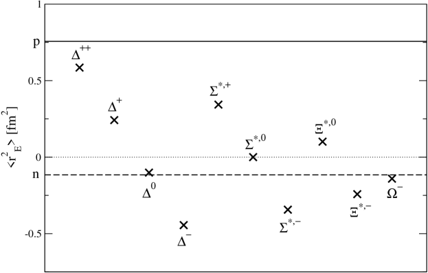
Figure 6.2: The charge radii of the decuplet baryons in $\chi$PT. The contribution from counterterms has been set to zero. The radii (squared) here come from the one-loop diagrams only and are plotted in units of fm². For reference we have shown both the proton and neutron charge radii [1] (solid and dashed lines, respectively).

6.2.2 Analysis in Q$\chi$PT

The calculation of the charge radii and electromagnetic moments can be correspondingly executed for Q$\chi$PT. The operators in Eqs. (6.7), (6.9) and (6.11) contribute, however, their low-energy coefficients cannot be matched onto QCD. Therefore we annotate them with a “Q”. The loop contributions encountered in $\chi$PT and PQ$\chi$PT above no longer contribute because in Q$\chi$PT $A^{T}_{X}=0$ for all decuplet states $T$. This can be readily seen in two ways. The quenched limit of the coefficients in Table 6.1 makes immediate the vanishing of $A_{X}^{T}$. Alternately one can consider the relevant quark flow diagrams with only valence quarks in loops. Due to the symmetric nature of $T^{ijk}$, these loops are completely canceled by their ghostly counterparts. For the charge radii, there are no additional diagrams to consider at this order from singlet hairpin interactions. Thus in Q$\chi$PT, the charge radii have the form

$$<r_{E}^{2}>=Q\left(\frac{2\mu_{c}^{Q}-1}{M_{B}^{2}}+\frac{\mathbb{Q}_{c}^{Q}+6c_{c}^{Q}}{{\Lambda}_{\chi}^{2}}\right),$$ (6.18)

where the dependence on the quark mass enters at the next order.

Additional terms of the form $\mu_{0}^{2}\log m_{q}$ involving hairpins [11, 13] do contribute to the electromagnetic moments as they are of the same order in the chiral expansion. As explained in [139], the axial hairpins do not contribute. In the diagrams shown in Fig. 6.3,

Figure 6.3: Hairpin diagrams that give contributions of the form $\sim\mu_{o}^{2}\log m_{q}$ to decuplet electromagnetic moments in Q$\chi$PT. The square at the photon vertex represents the relevant operators from Eqs. (6.7), (6.9), and (6.2.2).

one sees that there are contributions from the electromagnetic moments of the decuplet and octet baryons as well as their transition moments. These interactions are described by the operators in Eqs. (6.7) and (6.9) (now with quenched coefficients) along with

$${\mathcal{L}} = \frac{ie}{2M_{B}}\left\{\mu_{\alpha}^{Q}\left({\overline{{\mathcal{B}}}}[S^{\mu},S^{\nu}]{\mathcal{B}}{\mathcal{Q}}\right)+\mu_{\beta}^{Q}\left({\overline{{\mathcal{B}}}}[S^{\mu},S^{\nu}]{\mathcal{Q}}{\mathcal{B}}\right)\right\}F_{\mu\nu}$$

$$+\sqrt{\frac{3}{2}}\mu_{T}^{Q}\frac{ie}{2M_{B}}\left[\left({\overline{{\mathcal{B}}}}S^{\mu}{\mathcal{Q}}{\mathcal{T}}^{\nu}\right)+\text{h.c.}\right]F_{\mu\nu}+\sqrt{\frac{3}{2}}\mathbb{Q}_{T}^{Q}\frac{e}{{\Lambda}_{\chi}^{2}}\left[\left({\overline{{\mathcal{B}}}}S^{\{\mu}{\mathcal{Q}}{\mathcal{T}}^{\nu\}}\right)+\text{h.c.}\right]v^{\alpha}\partial_{\mu}F_{\nu{\alpha}}.$$

It is easier to work with the combinations $\mu_{D}^{Q}$ and $\mu_{F}^{Q}$ defined by

$$\mu_{\alpha}^{Q}=\frac{2}{3}\mu_{D}^{Q}+2\mu_{F}^{Q}\quad\text{and}\;\;\mu_{\beta}^{Q}=-\frac{5}{3}\mu_{D}^{Q}+\mu_{F}^{Q}.$$ (6.20)

To calculate the quenched electromagnetic moments, we also need the hairpin wavefunction renormalization diagrams shown in Fig. 6.1. These along with the diagrams in Fig. 6.3 are economically expressed in terms of the function

$$I(m_{1},m_{2},{\Delta}_{1},{\Delta}_{2},\mu) =\frac{Y(m_{1},{\Delta}_{1},\mu)+Y(m_{2},{\Delta}_{2},\mu)-Y(m_{1},{\Delta}_{2},\mu)-Y(m_{2},{\Delta}_{1},\mu)}{(m_{1}^{2}-m_{2}^{2})({\Delta}_{1}-{\Delta}_{2})}$$

$$=-i\frac{16\pi^{2}}{3}\int\frac{d^{D}k}{(2\pi)^{D}}\frac{k^{2}-(k\cdot v)^{2}}{(k^{2}-m_{1}^{2})(k^{2}-m_{2}^{2})(k\cdot v-{\Delta}_{1})(k\cdot v-{\Delta}_{2})},$$ (6.21)

where

$$Y(m,{\Delta},\mu)={\Delta}\left(m^{2}-\frac{2}{3}{\Delta}^{2}\right)\log\frac{m^{2}}{\mu^{2}}+\frac{2}{3}m({\Delta}^{2}-m^{2})\mathcal{R}\left(\frac{{\Delta}}{m}\right)$$ (6.22)

and we have kept only non-analytic contributions. The following shorthands are convenient

$$I_{\eta_{q}\eta_{q^{\prime}}} =I(m_{\eta_{q}},m_{\eta_{q^{\prime}}},0,0,\mu),$$

$$I^{{\Delta}}_{\eta_{q}\eta_{q^{\prime}}} =I(m_{\eta_{q}},m_{\eta_{q^{\prime}}},{\Delta},0,\mu),$$

$$I^{{\Delta}{\Delta}}_{\eta_{q}\eta_{q^{\prime}}} =I(m_{\eta_{q}},m_{\eta_{q^{\prime}}},{\Delta},{\Delta},\mu).$$ (6.23)

Specific limits of the function $I_{\eta_{q}\eta_{q^{\prime}}}$ appear in [13]. The wavefunction renormalization factors arising from hairpin diagrams can then be expressed as

$$Z=1-\frac{\mu_{o}^{2}}{16\pi^{2}f^{2}}\sum_{XX^{\prime}}\left[\frac{1}{2}(\mathcal{C}^{Q})^{2}C_{XX^{\prime}}I_{XX^{\prime}}+\frac{5}{9}(\mathcal{H}^{Q})^{2}B_{XX^{\prime}}I^{{\Delta}{\Delta}}_{XX^{\prime}}\right].$$ (6.24)

The coefficients $B_{XX^{\prime}}$ and $C_{XX^{\prime}}$ are listed in Table 6.2.

Table 6.2: The SU$(3)$ coefficients $B_{XX^{\prime}}$ and $C_{XX^{\prime}}$ in Q$\chi$PT.

	$B_{XX^{\prime}}$			$C_{XX^{\prime}}$
	$\quad\eta_{u}\eta_{u}$	$\quad\eta_{u}\eta_{s}$	$\quad\eta_{s}\eta_{s}$	$\quad\eta_{u}\eta_{u}$	$\quad\eta_{u}\eta_{s}$	$\quad\eta_{s}\eta_{s}$
$\Delta^{++},\Delta^{+},\Delta^{0},\Delta^{-}$	$1$	$0$	$0$	$0$	$0$	$0$
$\Sigma^{*,+},\Sigma^{*,0},\Sigma^{*,-}$	$\frac{4}{9}$	$\frac{4}{9}$	$\frac{1}{9}$	$\frac{2}{9}$	$-\frac{4}{9}$	$\frac{2}{9}$
$\Xi^{*,0},\Xi^{*,-}$	$\frac{1}{9}$	$\frac{4}{9}$	$\frac{4}{9}$	$\frac{2}{9}$	$-\frac{4}{9}$	$\frac{2}{9}$
$\Omega^{-}$	$0$	$0$	$1$	$0$	$0$	$0$

The sum in Eq. (6.24) is over $XX^{\prime}=\eta_{u}\eta_{u}$, $\eta_{u}\eta_{s}$, $\eta_{s}\eta_{s}$. Combining these factors with the tree-level contributions and including the corrections from the diagrams in Fig. 6.3, we arrive at the quenched decuplet magnetic moment

$$\mu = 2\mu_{c}^{Q}QZ+\frac{\mu_{o}^{2}}{16\pi^{2}f^{2}}\sum_{XX^{\prime}}\left[\frac{1}{2}(Q\mu_{F}^{Q}+{\alpha}_{D}\mu_{D}^{Q})(\mathcal{C}^{Q})^{2}C_{XX^{\prime}}I_{XX^{\prime}}\right]$$ (6.25)

$$+\frac{\mu_{o}^{2}}{16\pi^{2}f^{2}}\sum_{XX^{\prime}}\left[\frac{22}{27}(\mathcal{H}^{Q})^{2}\mu_{c}^{Q}B_{XX^{\prime}}QI^{{\Delta}{\Delta}}_{XX^{\prime}}-\frac{2}{9}\mathcal{C}^{Q}\mathcal{H}^{Q}\mu_{T}^{Q}D_{XX^{\prime}}I^{\Delta}_{XX^{\prime}}\right]$$

and the quenched electric quadrupole moment

$$\mathbb{Q} = -2Q\left(\mu_{c}^{Q}+\mathbb{Q}_{c}^{Q}\frac{2M_{B}^{2}}{{\Lambda}_{\chi}^{2}}\right)Z-\frac{\mu_{o}^{2}}{16\pi^{2}f^{2}}\frac{M_{B}^{2}}{{\Lambda}_{\chi}^{2}}\sum_{XX^{\prime}}\left(\frac{8}{3}\mathcal{C}^{Q}\mathcal{H}^{Q}\mathbb{Q}_{T}^{Q}D_{XX^{\prime}}I^{\Delta}_{XX^{\prime}}\right)$$

$$-\frac{\mu_{o}^{2}}{16\pi^{2}f^{2}}\sum_{XX^{\prime}}\left[(\mathcal{H}^{Q})^{2}\left(\frac{2}{9}\mu_{c}^{Q}+\frac{4}{9}\mathbb{Q}_{c}^{Q}\frac{M_{B}^{2}}{{\Lambda}_{\chi}^{2}}\right)QB_{XX^{\prime}}I^{{\Delta}{\Delta}}_{XX^{\prime}}-\frac{2}{3}\mathcal{C}^{Q}\mathcal{H}^{Q}\mu_{T}^{Q}D_{XX^{\prime}}I^{\Delta}_{XX^{\prime}}\right].$$

In Eq. (6.25) the required values for the constant ${\alpha}_{D}$ are: ${\alpha}_{D}=\frac{1}{3}$ for $\Sigma^{*,+}$, $\Sigma^{*,0}$, $\Sigma^{*,-}$, and $\Xi^{*,-}$, and ${\alpha}_{D}=-\frac{2}{3}$ for $\Xi^{*,0}$. The coefficients $D_{XX^{\prime}}$ are listed in Table 6.3.

Table 6.3: The SU$(3)$ coefficients $D_{XX^{\prime}}$ in Q$\chi$PT. Decuplet states not listed have $D_{XX^{\prime}}=0$.

	$\quad\eta_{u}\eta_{u}$	$\quad\eta_{u}\eta_{s}$	$\quad\eta_{s}\eta_{s}$
$\Sigma^{*,+}$	$\frac{2}{9}$	$-\frac{1}{9}$	$-\frac{1}{9}$
$\Sigma^{*,0}$	$\frac{1}{9}$	$-\frac{1}{18}$	$-\frac{1}{18}$
$\Xi^{*,0}$	$\frac{1}{9}$	$\frac{1}{9}$	$-\frac{2}{9}$

If a particular decuplet state is not listed, the value of $D_{XX^{\prime}}$ is zero for all singlet pairs $XX^{\prime}$.

The above expressions can be used to properly extrapolate quenched lattice data to the physical pion mass. For example, the expression for the quenched magnetic moments for the ${\Delta}$ baryons [Eq. (6.25)] reduces to

$$\mu=2Q\mu_{c}^{Q}\left(1-\frac{4}{27}\,\frac{\mu_{o}^{2}}{16\pi^{2}f^{2}}(\mathcal{H}^{Q})^{2}I^{{\Delta}{\Delta}}_{\eta_{u}\eta_{u}}\right).$$ (6.27)

In the above expression we need

$$I^{{\Delta}{\Delta}}_{XX}=\log\frac{m_{X}^{2}}{\mu^{2}}-\frac{{\Delta}m_{X}}{{\Delta}^{2}-m_{X}^{2}}{\mathcal{R}}\left(\frac{{\Delta}}{m_{X}}\right)+\dots.$$ (6.28)

where the ellipses denote terms analytic in $m_{X}$. Utilizing a least squares analysis and using the values $\mu=1$ GeV and ${\Delta}=270$ MeV , we extrapolate the quenched lattice data [129] to the physical pion mass and find for the ${\Delta}$ resonances

$$\mu=2.89\,Q\;[\mu_{N}].$$ (6.29)

This is in contrast to the value $\mu\approx 2.49\,Q\;[\mu_{N}]$ found from carrying out a $\chi$PT-type extrapolation [140]. Notice that for many of the decuplet states, in particular the ${\Delta}$ baryons, the quenched magnetic moments and electric quadrupole moments are proportional to the charge $Q$ (unlike the $\chi$PT and PQ$\chi$PT results). This elucidates the trends seen in the quenched lattice data [129].

6.3 Conclusions

We have calculated the electromagnetic moments and charge radii for the SU($3$) decuplet baryons in the isospin limit of PQ$\chi$PT and also derived the result for the baryon quartet away from the isospin limit for the $SU(2)$ chiral Lagrangian. The $q^{2}$ dependence of decuplet form factors at one-loop appears in Appendix E.1. We have also calculated the Q$\chi$PT results.

For the decuplet baryons’ electromagnetic moments and charge radii, the operators, which are included in the Q$\chi$PT but not in the $\chi$PT Lagrangian, enter at NNLO in the Q$\chi$PT expansion. Hence, formally our NLO result is not more divergent than its QCD counterpart. This, however, does not mean that our result is free of quenching artifacts. While the expansions about the chiral limit for QCD and QQCD charge radii are formally similar, $<r^{2}>\sim{\alpha}+{\beta}\log m_{Q}+\dots$, the QQCD result consists entirely of quenched oddities: for all decuplet baryons, diagrams that have bosonic or fermionic mesons running in loops completely cancel so that ${\beta}=0$. In other words, the quenched decuplet charge radii have the behavior $<r^{2}>\sim{\alpha}+\dots$ and the result is actually independent of $m_{Q}$ at this order. For the quenched decuplet magnetic moments and electric quadrupole moments, expansions about the chiral limit are again formally similar: $\mu\sim{\alpha}+{\beta}\log m_{Q}+\gamma\sqrt{m_{Q}}+\ldots$ and $\mathbb{Q}\sim{\alpha}+{\beta}\log m_{Q}+\ldots$. However, quenching forces $\gamma=0$ and both ${\beta}$’s arise from singlet contributions involving the parameter $\mu_{o}$, which is of course absent in QCD. Thus the leading non-analytic quark mass dependence that remains for these observables is entirely a quenched peculiarity.

PQQCD, on the other hand, is free of such excentric behavior and our PQ$\chi$PT result will enable the proper extrapolation of PQQCD lattice simulations of the decuplet electromagnetic moments and charge radii and we hope it encourages such simulations in the future.

Chapter 7 Baryon Decuplet to Octet Electromagnetic Transitions in Q$\chi$PT and PQ$\chi$PT

In this chapter, we calculate baryon decuplet to octet electromagnetic transition form factors in quenched and partially quenched chiral perturbation theory. Again, we work in the isospin limit of $SU(3)$ flavor, up to NLO in the chiral expansion, and to leading order in the heavy baryon expansion. Our results are necessary for proper extrapolation of lattice calculations of these transitions. We also derive expressions for the case of $SU(2)$ flavor away from the isospin limit.

7.1 Introduction

The study of the baryon decuplet to octet electromagnetic transitions provides important insight into the strongly interacting regime of QCD. Spin-parity selection rules for these transitions allow for magnetic dipole (M1), electric quadrupole (E2), and Coulumb quadrupole (C2) amplitudes. Understanding these amplitudes, both in theory and experiment, gives insight into the ground state wavefunctions of the lowest lying baryons. For example, in the transition of the ${\Delta}(1232)$ to the nucleon, if both baryon wavefunctions are spherically symmetric then the E2 and C2 amplitudes vanish. Experimentally, M1 is seen to be the dominant amplitude. However, recent experimental measurements of the quadrupole amplitudes in the ${\Delta}\to N{\gamma}$ transition [141, 142] show that the quadrupole amplitudes E2 and C2 are likely non-zero. This has revitalized the discussion as to the mechanism for deformation of the baryons. Although we expect more experimental data in the future, progress will be slower for the remaining transitions as the experimental difficulties are large.

First-principle lattice QCD calculations of these matrix elements can provide a theoretical explanation of these experimental results. In fact, the experimental difficulties may force us to rely on lattice data for the non-nucleonic transitions. Recently several such lattice calculations [143, 144], which improve upon an earlier one [145], have appeared. Unfortunately now and foreseeably, these lattice calculations cannot be performed with the physical masses of the light quarks and must be extrapolated to the physical light quark masses.

For future lattice calculations that use the partially quenched approximation of QCD one needs to fit PQ$\chi$PT to the lattice data in order to determine the low-energy constants and to actually make physical predictions for QCD. Unfortunately, partially quenched simulations for the ${\Delta}\to N{\gamma}$ transition do not exist yet; what does exist are simulations [143, 144] that use the quenched approximation. These simulations must be fit using Q$\chi$PT that exhibit the sickness outlined in the previous chapters. However, we expect to see partially quenched calculations of these form factors in the near future.

This chapter is organized as follows. In Section 7.2 we calculate baryon decuplet to octet transition form factors in both Q$\chi$PT and PQ$\chi$PT up to NLO in the chiral expansion and keep contributions to lowest order in the heavy baryon mass, $M_{B}$. These calculations are done in the isospin limit of $SU(3)$ flavor. For completeness we also provide the PQ$\chi$PT results for the transitions using the $SU(2)$ chiral Lagrangian with non-degenerate quarks in Appendix F. In Section 7.3 we conclude.

7.2 Baryon Decuplet to Octet Transition

The electromagnetic baryon decuplet to octet transitions have been investigated previously in $\chi$PT [146, 147, 148, 149]. Very recently there also has been renewed interest in these transitions in the large $N_{c}$ limit of QCD [150]. Here we calculate these transitions in PQ$\chi$PT and Q$\chi$PT. While we have reviewed PQ$\chi$PT briefly in the last section and our recent papers [4, 5], for Q$\chi$PT we refer the reader to the literature [17, 18, 20, 19, 21, 48, 11].

Using the heavy baryon formalism [115, 33], transition matrix elements of the electromagnetic current $J^{\rho}$ between a decuplet baryon with momentum $p^{\prime}$ and an octet baryon with momentum $p$ can be parametrized as

$$\langle{{\overline{B}}}(p)|J^{\rho}|T(p^{\prime})\rangle={{\overline{u}}}(p){\mathcal{O}}^{\rho\mu}u_{\mu}(p^{\prime}),$$ (7.1)

where $u_{\mu}(p)$ is a Rarita-Schwinger spinor for an on-shell decuplet baryon satisfying $v^{\mu}u_{\mu}(p)=0$ and $S^{\mu}u_{\mu}(p)=0$. The tensor ${\mathcal{O}}^{\rho\mu}$ can be parametrized in terms of three independent, Lorentz invariant, dimensionless form factors [151]

$$\mathcal{O}^{\rho\mu} = \frac{G_{1}(q^{2})}{M_{B}}\left(q\cdot Sg^{\mu\rho}-q^{\mu}S^{\rho}\right)+\frac{G_{2}(q^{2})}{(2M_{B})^{2}}\left(q\cdot vg^{\mu\rho}-q^{\mu}v^{\rho}\right)S\cdot q$$ (7.2)

$$+\frac{G_{3}(q^{2})}{4M_{B}^{2}{\Delta}}\left(q^{2}g^{\mu\rho}-q^{\mu}q^{\rho}\right)S\cdot q,$$

where the momentum of the outgoing photon is $q=p^{\prime}-p$. Here we have adopted the normalization of the $G_{3}(q^{2})$ form factor used in [149] so that the leading contributions to all three form factors are of order unity in the power counting.

Linear combinations of the above form factors at $q^{2}=0$ make the magnetic dipole, electric quadrupole, and Coulombic quadrupole moments,

$$G_{M1}(0) = \left(\frac{2}{3}-\frac{{\Delta}}{6M_{B}}\right)G_{1}(0)+\frac{{\Delta}}{12M_{B}}G_{2}(0),$$

$$G_{E2}(0) = \frac{{\Delta}}{6M_{B}}G_{1}(0)+\frac{{\Delta}}{12M_{B}}G_{2}(0),$$

$$G_{C2}(0) = \left(\frac{1}{3}+\frac{{\Delta}}{6M_{B}}\right)G_{1}(0)+\left(\frac{1}{6}+\frac{{\Delta}}{6M_{B}}\right)G_{2}(0)+\frac{1}{6}G_{3}(0).$$ (7.3)

Analysis in PQ$\chi$PT

Let us first consider the transition form factors in PQ$\chi$PT. Here, the leading tree-level contributions to the transition moments come from the dimension-5 and dimension-6 operators

$${\mathcal{L}}=\sqrt{\frac{3}{2}}\mu_{T}\frac{ie}{2M_{B}}\left({\overline{{\mathcal{B}}}}S^{\mu}{\mathcal{Q}}{\mathcal{T}}^{\nu}\right)F_{\mu\nu}+\sqrt{\frac{3}{2}}\mathbb{Q}_{T}\frac{e}{{\Lambda}_{\chi}^{2}}\left({\overline{{\mathcal{B}}}}S^{\{\mu}{\mathcal{Q}}{\mathcal{T}}^{\nu\}}\right)v^{\alpha}\partial_{\mu}F_{\nu{\alpha}}$$ (7.4)

where the action of ${}^{\{}\ldots{}^{\}}$ on Lorentz indices produces the symmetric traceless part of the tensor, viz., $\mathcal{O}^{\{\mu\nu\}}=\mathcal{O}^{\mu\nu}+\mathcal{O}^{\nu\mu}-\frac{1}{2}g^{\mu\nu}\mathcal{O}^{\alpha}{}_{\alpha}$. Here the PQQCD low-energy constants $\mu_{T}$ and $\mathbb{Q}_{T}$ have the same numerical values as in QCD.

The NLO contributions in the chiral expansion arise from the one-loop diagrams shown in Figs. (7.1) and (7.2).

Figure 7.1: Loop diagrams that contribute to the transition moments but are zero to the order we are working. A thin (thick) solid line denotes an octet (decuplet) baryon whereas a dashed line denotes a meson.

Figure 7.2: Loop diagrams contributing to the transition moments

However, because of the constraints satisfied by the on-shell Rarita-Schwinger spinors, the diagrams in Fig. (7.1) are all identically zero. For the calculation of the diagrams in Fig. (7.2) we need the terms in the Lagrangian describing the interaction of the ${\mathcal{B}}_{ijk}$ and ${\mathcal{T}}_{ijk}$ with the pseudo-Goldstone mesons given in Eqs. (5.17) and (6.13):

$${\cal L}=2{\alpha}\left({\overline{{\mathcal{B}}}}S^{\mu}{\mathcal{B}}A_{\mu}\right)+2{\beta}\left({\overline{{\mathcal{B}}}}S^{\mu}A_{\mu}{\mathcal{B}}\right)+\sqrt{\frac{3}{2}}{\mathcal{C}}\left[\left({\overline{{\mathcal{T}}}}^{\nu}A_{\nu}{\mathcal{B}}\right)+\text{h.c.}\right]+2{\mathcal{H}}\left({\overline{{\mathcal{T}}}}^{\nu}S^{\mu}A_{\mu}{\mathcal{T}}_{\nu}\right).$$ (7.5)

We find

$$G_{1}(0) = \frac{\mu_{T}}{2}{\alpha}_{T}+\frac{M_{B}}{{\Lambda}_{\chi}^{2}}4{\mathcal{H}}{\mathcal{C}}\sum_{X}{\beta}_{X}^{T}\int_{0}^{1}dx\,\left(1-\frac{x}{3}\right)\left[x{\Delta}\log\frac{m_{X}^{2}}{\mu^{2}}-m_{X}{\mathcal{R}}\left(\frac{x{\Delta}}{m_{X}}\right)\right]$$

$$-\frac{M_{B}}{{\Lambda}_{\chi}^{2}}4{\mathcal{C}}(D-F)\sum_{X}{\beta}_{X}^{B}\int_{0}^{1}dx\,(1-x)\left[x{\Delta}\log\frac{m_{X}^{2}}{\mu^{2}}+m_{X}{\mathcal{R}}\left(-\frac{x{\Delta}}{m_{X}}\right)\right],$$

$$G_{2}(0) = \frac{M_{B}^{2}}{{\Lambda}_{\chi}^{2}}\Bigg{\{}-4\mathbb{Q}_{T}{\alpha}_{T}$$

$$\phantom{xxxxx}+16{\mathcal{H}}{\mathcal{C}}\sum_{X}{\beta}_{X}^{T}\int_{0}^{1}dx\,\frac{x(1-x)}{3}\left[\log\frac{m_{X}^{2}}{\mu^{2}}+\frac{x{\Delta}m_{X}}{m_{X}^{2}-x^{2}{\Delta}^{2}}{\mathcal{R}}\left(\frac{x{\Delta}}{m_{X}}\right)\right]$$

$$-16{\mathcal{C}}(D-F)\sum_{X}{\beta}_{X}^{B}\int_{0}^{1}dx\,x(1-x)\left[\log\frac{m_{X}^{2}}{\mu^{2}}-\frac{x{\Delta}m_{X}}{m_{X}^{2}-x^{2}{\Delta}^{2}}{\mathcal{R}}\left(-\frac{x{\Delta}}{m_{X}}\right)\right]\Bigg{\}},$$

and

$$G_{3}(0) = -\frac{M_{B}^{2}}{{\Lambda}_{\chi}^{2}}16\left[{\mathcal{H}}{\mathcal{C}}\sum_{X}{\beta}_{X}^{T}\int_{0}^{1}dx\,\frac{x(1-x)}{3}\left(x-\frac{1}{2}\right)\frac{{\Delta}m_{X}}{m_{X}^{2}-x^{2}{\Delta}^{2}}{\mathcal{R}}\left(\frac{x{\Delta}}{m_{X}}\right)\right.$$

$$\left.+{\mathcal{C}}(D-F)\sum_{X}{\beta}_{X}^{B}\int_{0}^{1}dx\,x(1-x)\left(x-\frac{1}{2}\right)\frac{{\Delta}m_{X}}{m_{X}^{2}-x^{2}{\Delta}^{2}}{\mathcal{R}}\left(-\frac{x{\Delta}}{m_{X}}\right)\right],$$

where the function $\mathcal{R}(x)$ is defined in Eq. (B.2) and we have only kept loop contributions that are non-analytic in the meson mass $m_{X}$. The tree-level coefficients ${\alpha}_{T}$ are listed in Table 7.1

Table 7.1: Tree-level coefficients ${\alpha}_{T}$ in $\chi$PT, Q$\chi$PT, and PQ$\chi$PT.

	${\alpha}_{T}$
${\Delta}\to N\gamma$	$\frac{1}{\sqrt{3}}$
$\Sigma^{*,+}\to\Sigma^{+}\gamma$	$-\frac{1}{\sqrt{3}}$
$\Sigma^{*,0}\to\Sigma^{0}\gamma$	$\frac{1}{2\sqrt{3}}$
$\Sigma^{*,0}\to\Lambda\gamma$	$-\frac{1}{2}$
$\Sigma^{*,-}\to\Sigma^{-}\gamma$	$0$
$\Xi^{*,0}\to\Xi^{0}\gamma$	$-\frac{1}{\sqrt{3}}$
$\Xi^{*,-}\to\Xi^{-}\gamma$	$0$

and the coefficients for the loop diagrams in Fig. (7.2), ${\beta}_{X}^{T}$ and ${\beta}_{X}^{B}$, are given in Tables 7.3 and 7.3, respectively.

Table 7.2: The $SU(3)$ coefficients $\beta_{X}^{T}$ in $\chi$PT and PQ$\chi$PT.

	$\chi$PT		PQ$\chi$PT
	$\pi$	$K$	$\pi$	$K$	$\eta_{s}$	$ju$	$ru$	$js$	$rs$
${\Delta}\to N\gamma$	$\frac{5}{3\sqrt{3}}$	$\frac{1}{3\sqrt{3}}$	$\frac{1}{\sqrt{3}}$	$0$	$0$	$\frac{2}{3\sqrt{3}}$	$\frac{1}{3\sqrt{3}}$	$0$	$0$
$\Sigma^{*,+}\to\Sigma^{+}\gamma$	$-\frac{1}{3\sqrt{3}}$	$-\frac{5}{3\sqrt{3}}$	$\frac{1-3q_{jl}}{9\sqrt{3}}$	$-\frac{11-3q_{jl}+3q_{r}}{9\sqrt{3}}$	$\frac{1+3q_{r}}{9\sqrt{3}}$	$-\frac{4-3q_{jl}}{9\sqrt{3}}$	$-\frac{2-3q_{r}}{9\sqrt{3}}$	$-\frac{2+3q_{jl}}{9\sqrt{3}}$	$-\frac{1+3q_{r}}{9\sqrt{3}}$
$\Sigma^{*,0}\to\Sigma^{0}\gamma$	$0$	$\frac{1}{\sqrt{3}}$	$-\frac{1-3q_{jl}}{9\sqrt{3}}$	$\frac{13-6q_{jl}+6q_{r}}{18\sqrt{3}}$	$-\frac{1+3q_{r}}{9\sqrt{3}}$	$\frac{1-3q_{jl}}{9\sqrt{3}}$	$\frac{1-6q_{r}}{18\sqrt{3}}$	$\frac{2+3q_{jl}}{9\sqrt{3}}$	$\frac{1+3q_{r}}{9\sqrt{3}}$
$\Sigma^{*,0}\to\Lambda\gamma$	$-\frac{2}{3}$	$-\frac{1}{3}$	$-\frac{1}{3}$	$-\frac{1}{6}$	$0$	$-\frac{1}{3}$	$-\frac{1}{6}$	$0$	$0$
$\Sigma^{*,-}\to\Sigma^{-}\gamma$	$-\frac{1}{3\sqrt{3}}$	$\frac{1}{3\sqrt{3}}$	$-\frac{1-3q_{jl}}{9\sqrt{3}}$	$\frac{2-3q_{jl}+3q_{r}}{9\sqrt{3}}$	$-\frac{1+3q_{r}}{9\sqrt{3}}$	$-\frac{2+3q_{jl}}{9\sqrt{3}}$	$-\frac{1+3q_{r}}{9\sqrt{3}}$	$\frac{2+3q_{jl}}{9\sqrt{3}}$	$\frac{1+3q_{r}}{9\sqrt{3}}$
$\Xi^{*,0}\to\Xi^{0}\gamma$	$-\frac{1}{3\sqrt{3}}$	$-\frac{5}{3\sqrt{3}}$	$\frac{1-3q_{jl}}{9\sqrt{3}}$	$-\frac{11-3q_{jl}+3q_{r}}{9\sqrt{3}}$	$\frac{1+3q_{r}}{9\sqrt{3}}$	$-\frac{4-3q_{jl}}{9\sqrt{3}}$	$-\frac{2-3q_{r}}{9\sqrt{3}}$	$-\frac{2+3q_{jl}}{9\sqrt{3}}$	$-\frac{1+3q_{r}}{9\sqrt{3}}$
$\Xi^{*,-}\to\Xi^{-}\gamma$	$-\frac{1}{3\sqrt{3}}$	$\frac{1}{3\sqrt{3}}$	$-\frac{1-3q_{jl}}{9\sqrt{3}}$	$\frac{2-3q_{jl}+3q_{r}}{9\sqrt{3}}$	$-\frac{1+3q_{r}}{9\sqrt{3}}$	$-\frac{2+3q_{jl}}{9\sqrt{3}}$	$-\frac{1+3q_{r}}{9\sqrt{3}}$	$\frac{2+3q_{jl}}{9\sqrt{3}}$	$\frac{1+3q_{r}}{9\sqrt{3}}$

Table 7.3: The $SU(3)$ coefficients $\beta_{X}^{B}$ in $\chi$PT and PQ$\chi$PT.

	$\chi$PT		PQ$\chi$PT
	$\pi$	$K$	$\pi$	$K$	$\eta_{s}$	$ju$	$ru$	$js$	$rs$
${\Delta}\to N\gamma$	$-\frac{D+F}{\sqrt{3}(D-F)}$	$-\frac{1}{\sqrt{3}}$	$\frac{D-3F}{\sqrt{3}(D-F)}$	$0$	$0$	$-\frac{2}{\sqrt{3}}$	$-\frac{1}{\sqrt{3}}$	$0$	$0$
$\Sigma^{*,+}\to\Sigma^{+}\gamma$	$\frac{1}{\sqrt{3}}$	$\frac{D+F}{\sqrt{3}(D-F)}$	$-\frac{1-3q_{jl}}{3\sqrt{3}}$	$-\frac{D-7F}{3\sqrt{3}(D-F)}+\frac{q_{jl}-q_{r}}{\sqrt{3}}$	$-\frac{1+3q_{r}}{3\sqrt{3}}$	$\frac{4-3q_{jl}}{3\sqrt{3}}$	$\frac{2-3q_{r}}{3\sqrt{3}}$	$\frac{2+3q_{jl}}{3\sqrt{3}}$	$\frac{1+3q_{r}}{3\sqrt{3}}$
$\Sigma^{*,0}\to\Sigma^{0}\gamma$	$0$	$-\frac{D}{\sqrt{3}(D-F)}$	$\frac{1-3q_{jl}}{3\sqrt{3}}$	$-\frac{D+5F}{6\sqrt{3}(D-F)}-\frac{q_{jl}-q_{r}}{\sqrt{3}}$	$\frac{1+3q_{r}}{3\sqrt{3}}$	$-\frac{1-3q_{jl}}{3\sqrt{3}}$	$-\frac{1-6q_{r}}{6\sqrt{3}}$	$-\frac{2+3q_{jl}}{3\sqrt{3}}$	$-\frac{1+3q_{r}}{3\sqrt{3}}$
$\Sigma^{*,0}\to\Lambda\gamma$	$\frac{2D}{3(D-F)}$	$\frac{D}{3(D-F)}$	$-\frac{D-3F}{3(D-F)}$	$-\frac{D-3F}{6(D-F)}$	$0$	$1$	$\frac{1}{2}$	$0$	$0$
$\Sigma^{*,-}\to\Sigma^{-}\gamma$	$\frac{1}{\sqrt{3}}$	$-\frac{1}{\sqrt{3}}$	$\frac{1-3q_{jl}}{3\sqrt{3}}$	$-\frac{2-3q_{jl}+3q_{r}}{3\sqrt{3}}$	$\frac{1+3q_{r}}{3\sqrt{3}}$	$\frac{2+3q_{jl}}{3\sqrt{3}}$	$\frac{1+3q_{r}}{3\sqrt{3}}$	$-\frac{2+3q_{jl}}{3\sqrt{3}}$	$-\frac{1+3q_{r}}{3\sqrt{3}}$
$\Xi^{*,0}\to\Xi^{0}\gamma$	$\frac{1}{\sqrt{3}}$	$\frac{D+F}{\sqrt{3}(D-F)}$	$-\frac{1-3q_{jl}}{3\sqrt{3}}$	$-\frac{D-7F}{3\sqrt{3}(D-F)}+\frac{q_{jl}-q_{r}}{\sqrt{3}}$	$-\frac{1+3q_{r}}{3\sqrt{3}}$	$\frac{4-3q_{jl}}{3\sqrt{3}}$	$\frac{2-3q_{r}}{3\sqrt{3}}$	$\frac{2+3q_{jl}}{3\sqrt{3}}$	$\frac{1+3q_{r}}{3\sqrt{3}}$
$\Xi^{*,-}\to\Xi^{-}\gamma$	$\frac{1}{\sqrt{3}}$	$-\frac{1}{\sqrt{3}}$	$\frac{1-3q_{jl}}{3\sqrt{3}}$	$-\frac{2-3q_{jl}+3q_{r}}{3\sqrt{3}}$	$\frac{1+3q_{r}}{3\sqrt{3}}$	$\frac{2+3q_{jl}}{3\sqrt{3}}$	$\frac{1+3q_{r}}{3\sqrt{3}}$	$-\frac{2+3q_{jl}}{3\sqrt{3}}$	$-\frac{1+3q_{r}}{3\sqrt{3}}$

In these tables we have listed values corresponding to the loop meson with mass $m_{X}$. As required, in the QCD limit the PQ$\chi$PT coefficients reduce to those of $\chi$PT. It is comforting that the one-loop results for the $G_{3}(q^{2})$ form factor are finite. This is consistent with the fact that one cannot write down a dimension-7 operator that contributes at the same order in the chiral expansion as our one-loop result for $G_{3}(q^{2})$. The full one-loop $q^{2}$ dependence of these form factors can easily be recovered by replacing

$$m_{X}\to\sqrt{m_{X}^{2}-x(1-x)q^{2}}.$$ (7.9)

Notice that the tree-level transitions ${\Sigma}^{*,-}\to{\Sigma}^{-}\gamma$ and $\Xi^{*,-}\to\Xi^{-}\gamma$ are zero because they are forbidden by $d\leftrightarrow s$ $U$-spin symmetry [152]. There is also symmetry between the ${\Sigma}^{*,+}\to{\Sigma}^{+}\gamma$ and $\Xi^{*,0}\to\Xi^{0}\gamma$ transitions as well as the ${\Sigma}^{*,-}\to{\Sigma}^{-}\gamma$ and $\Xi^{*,-}\to\Xi^{-}\gamma$ transitions that holds to NLO in $\chi$PT and PQ$\chi$PT.

Analysis in Q$\chi$PT

The calculation of the transition moments can be repeated in Q$\chi$PT. At tree level, the operators in Eq. (7.4) contribute, but their low-energy coefficients cannot be matched onto QCD. Therefore we annotate them with a “Q”. At the next order in the chiral expansion, there are again contributions from the loop diagrams in Fig. (7.2). The results are the same as in the partially quenched theory, Eqs. (7.2)–(7.2), with the coefficients ${\beta}_{X}^{T}$ and ${\beta}_{X}^{B}$ replaced by ${\beta}_{X}^{T,Q}$ and ${\beta}_{X}^{B,Q}/(D^{Q}-F^{Q})$, which are listed in Table 7.4.

Table 7.4: The $SU(3)$ coefficients $\beta_{X}^{B,Q}$ and $\beta_{X}^{T,Q}$ in Q$\chi$PT.

	$\beta_{X}^{T,Q}$		$\beta_{X}^{B,Q}$
	$\pi$	$K$	$\pi$	$K$
${\Delta}\to N\gamma$	$\frac{1}{\sqrt{3}}$	$0$	$\frac{1}{\sqrt{3}}(D^{Q}-3F^{Q})$	$0$
$\Sigma^{*,+}\to\Sigma^{+}\gamma$	$0$	$-\frac{1}{\sqrt{3}}$	$0$	$-\frac{1}{\sqrt{3}}(D^{Q}-3F^{Q})$
$\Sigma^{*,0}\to\Sigma^{0}\gamma$	$0$	$\frac{1}{2\sqrt{3}}$	$0$	$\frac{1}{2\sqrt{3}}(D^{Q}-3F^{Q})$
$\Sigma^{*,0}\to\Lambda\gamma$	$-\frac{1}{3}$	$-\frac{1}{6}$	$-\frac{1}{3}(D^{Q}-3F^{Q})$	$-\frac{1}{6}(D^{Q}-3F^{Q})$
$\Sigma^{*,-}\to\Sigma^{-}\gamma$	$0$	$0$	$0$	$0$
$\Xi^{*,0}\to\Xi^{0}\gamma$	$0$	$-\frac{1}{\sqrt{3}}$	$0$	$-\frac{1}{\sqrt{3}}(D^{Q}-3F^{Q})$
$\Xi^{*,-}\to\Xi^{-}\gamma$	$0$	$0$	$0$	$0$

In addition, there are contributions of the form $\mu_{0}^{2}\log m_{q}$ at the same order in the chiral expansion that are artifacts of quenching. These come from hairpin wavefunction renormalization diagrams and from the four loop diagrams in Fig. (7.3).

Figure 7.3: Loop diagrams contributing to the transition form factors in Q$\chi$PT. The four diagrams correspond to terms involving the parameters $A_{XX^{\prime}}$, $B_{XX^{\prime}}$, $C_{XX^{\prime}}$, and $D_{XX^{\prime}}$ in Eqs. (7.2) and (7.14).

In these diagrams the photon can couple to the baryon line via

$${\cal L} = \frac{ie}{2M_{B}}\left[\mu_{\alpha}^{Q}\left({\overline{{\mathcal{B}}}}[S_{\mu},S_{\nu}]{\mathcal{B}}{\mathcal{Q}}\right)+\mu_{\beta}^{Q}\left({\overline{{\mathcal{B}}}}[S_{\mu},S_{\nu}]{\mathcal{Q}}{\mathcal{B}}\right)\right]F^{\mu\nu}$$ (7.10)

$$+\mu_{c}^{Q}\frac{3ie}{M_{B}}\big{(}{\overline{{\mathcal{T}}}}_{\mu}{\mathcal{Q}}{\mathcal{T}}_{\nu}\big{)}F^{\mu\nu}-\mathbb{Q}_{\text{c}}^{Q}\frac{3e}{{\Lambda}_{\chi}^{2}}\big{(}{\overline{{\mathcal{T}}}}{}^{\{\mu}{\mathcal{Q}}{\mathcal{T}}^{\nu\}}\big{)}v^{\alpha}\partial_{\mu}F_{\nu\alpha}$$

and via the terms in Eq. (7.4) including their hermitian conjugates (with quenched coefficients). It is easier to work with the combinations $\mu_{D}^{Q}$ and $\mu_{F}^{Q}$ defined by

$$\mu_{\alpha}^{Q}=\frac{2}{3}\mu_{D}^{Q}+2\mu_{F}^{Q}\quad\text{and}\quad\mu_{\beta}^{Q}=-\frac{5}{3}\mu_{D}^{Q}+\mu_{F}^{Q}.$$ (7.12)

Although the argument presented in [139] does not apply to the case of different initial and final states, the axial hairpin interactions still do not contribute simply because their presence requires closed quark loops. The hairpin wavefunction renormalization diagrams have been calculated in Q$\chi$PT for the baryon octet [13] ($Z^{Q}_{B}$) and decuplet [5] ($Z^{Q}_{T}$) and we do not reproduce them here. We find the hairpin contributions to the transition form factors to be

$$G^{HP}_{1}(q^{2}) = \frac{\mu_{T}^{Q}}{2}{\alpha}_{T}\frac{Z_{B}^{Q}-1}{2}\frac{Z_{T}^{Q}-1}{2}$$

$$+\frac{\mu_{0}^{2}}{16\pi^{2}f^{2}}\sum_{X,X^{\prime}}\Bigg{[}\frac{5}{108}{\mathcal{H}}^{Q}\mu_{T}^{Q}A_{XX^{\prime}}I_{XX^{\prime}}-\frac{1}{18}\left({\mathcal{C}}^{Q}\right)^{2}\mu_{T}^{Q}B_{XX^{\prime}}I_{XX^{\prime}}^{-{\Delta},{\Delta}}$$

$$\phantom{xxxx}-\frac{20}{27}{\mathcal{H}}^{Q}{\mathcal{C}}^{Q}Q_{T}\mu_{c}^{Q}C_{XX^{\prime}}I_{XX^{\prime}}^{\Delta}-\frac{2}{3}{\mathcal{C}}^{Q}\left(Q_{T}\mu_{F}^{Q}+{\alpha}_{D}\mu_{D}^{Q}\right)D_{XX^{\prime}}I^{{\Delta}}_{XX^{\prime}}\Bigg{]},$$

$$G^{HP}_{2}(q^{2}) = -4{\mathbb{Q}}_{T}^{Q}{\alpha}_{T}\frac{M_{B}^{2}}{{\Lambda}_{\chi}^{2}}\frac{Z_{B}^{Q}-1}{2}\frac{Z_{T}^{Q}-1}{2}$$ (7.14)

$$+\frac{\mu_{0}^{2}}{16\pi^{2}f^{2}}\frac{M_{B}^{2}}{{\Lambda}_{\chi}^{2}}\sum_{XX^{\prime}}\Bigg{[}\frac{2}{9}{\mathcal{H}}^{Q}{\mathbb{Q}}_{T}^{Q}A_{XX^{\prime}}I_{XX^{\prime}}+\frac{4}{3}\left(C^{Q}\right)^{2}{\mathbb{Q}}_{T}^{Q}B_{XX^{\prime}}I^{-{\Delta}\,{\Delta}}_{XX^{\prime}}$$

$$\phantom{xxxxxxxxxxxxxxxx}-\frac{16}{9}{\mathcal{H}}^{Q}{\mathcal{C}}^{Q}Q_{T}{\mathbb{Q}}_{C}^{Q}C_{XX^{\prime}}I^{\Delta}_{XX^{\prime}}\Bigg{]},$$

and $G^{HP}_{3}(q^{2})=0$. Thus in Q$\chi$PT: $G_{j}^{Q}(q^{2})=G_{j}^{PQ}(q^{2})+G_{j}^{HP}(q^{2})$, where the ${\beta}_{X}^{T}$ and ${\beta}_{X}^{B}$ coefficients of $G_{j}^{PQ}(q^{2})$, Eqs. (7.2)–(7.2), are understood to be replaced by their quenched values ${\beta}_{X}^{T,Q}$ and ${\beta}_{X}^{B,Q}/(D^{Q}-F^{Q})$. Above we have used the shorthand notation $I_{\eta_{q}\eta_{q^{\prime}}}=I(m_{\eta_{q}},m_{\eta_{q^{\prime}}},0,0,\mu)$, $I^{{\Delta}}_{\eta_{q}\eta_{q^{\prime}}}=I(m_{\eta_{q}},m_{\eta_{q^{\prime}}},{\Delta},0,\mu)$, and $I^{{\Delta}_{1},{\Delta}_{2}}_{\eta_{q}\eta_{q^{\prime}}}=I(m_{\eta_{q}},m_{\eta_{q^{\prime}}},{\Delta}_{1},{\Delta}_{2},\mu)$ for the function $I(m_{1},m_{2},{\Delta}_{1},{\Delta}_{2},\mu)$ that is given by

$$I(m_{1},m_{2},{\Delta}_{1},{\Delta}_{2},\mu)=\frac{Y(m_{1},{\Delta}_{1},\mu)+Y(m_{2},{\Delta}_{2},\mu)-Y(m_{1},{\Delta}_{2},\mu)-Y(m_{2},{\Delta}_{1},\mu)}{(m_{1}^{2}-m_{2}^{2})({\Delta}_{1}-{\Delta}_{2})}$$ (7.15)

with

$$Y(m,{\Delta},\mu)={\Delta}\left(m^{2}-\frac{2}{3}{\Delta}^{2}\right)\log\frac{m^{2}}{\mu^{2}}+\frac{2}{3}m({\Delta}^{2}-m^{2})\mathcal{R}\left(\frac{{\Delta}}{m}\right).$$ (7.16)

The coefficients $A_{XX^{\prime}}$, $B_{XX^{\prime}}$, $C_{XX^{\prime}}$, and $D_{XX^{\prime}}$ are listed in Tables 7.5 and 7.6.

Table 7.5: The $SU(3)$ coefficients $A_{XX^{\prime}}$ and $B_{XX^{\prime}}$ in Q$\chi$PT.

	$A_{XX^{\prime}}$			$B_{XX^{\prime}}$
	$\eta_{u}\eta_{u}$	$\eta_{u}\eta_{s}$	$\eta_{s}\eta_{s}$	$\eta_{u}\eta_{u}$	$\eta_{u}\eta_{s}$	$\eta_{s}\eta_{s}$
${\Delta}\to N\gamma$	$2\sqrt{3}(D^{Q}-3F^{Q})$	$0$	$0$	$0$	$0$	$0$
$\Sigma^{*,+}\to\Sigma^{+}\gamma$	$\frac{8}{\sqrt{3}}F^{Q}$	$-\frac{4}{\sqrt{3}}(D^{Q}-2F^{Q})$	$-\frac{2}{\sqrt{3}}(D^{Q}-F^{Q})$	$\frac{1}{3\sqrt{3}}$	$-\frac{2}{3\sqrt{3}}$	$\frac{1}{3\sqrt{3}}$
$\Sigma^{*,0}\to\Sigma^{0}\gamma$	$-\frac{4}{\sqrt{3}}F^{Q}$	$\frac{2}{\sqrt{3}}(D^{Q}-2F^{Q})$	$\frac{1}{\sqrt{3}}(D^{Q}-F^{Q})$	$-\frac{1}{6\sqrt{3}}$	$\frac{1}{3\sqrt{3}}$	$-\frac{1}{6\sqrt{3}}$
$\Sigma^{*,0}\to\Lambda\gamma$	$-\frac{4}{3}(2D^{Q}-3F^{Q})$	$-\frac{2}{3}(D^{Q}-6F^{Q})$	$\frac{1}{3}(D^{Q}+3F^{Q})$	$0$	$0$	$0$
$\Sigma^{*,-}\to\Sigma^{-}\gamma$	$0$	$0$	$0$	$0$	$0$	$0$
$\Xi^{*,0}\to\Xi^{0}\gamma$	$-\frac{2}{\sqrt{3}}(D^{Q}-F^{Q})$	$-\frac{4}{\sqrt{3}}(D^{Q}-2F^{Q})$	$\frac{8}{\sqrt{3}}F^{Q}$	$\frac{1}{3\sqrt{3}}$	$-\frac{2}{3\sqrt{3}}$	$\frac{1}{3\sqrt{3}}$
$\Xi^{*,-}\to\Xi^{-}\gamma$	$0$	$0$	$0$	$0$	$0$	$0$

Table 7.6: The $SU(3)$ coefficients $C_{XX^{\prime}}$ and $D_{XX^{\prime}}$ in Q$\chi$PT.

	$C_{XX^{\prime}}$			$D_{XX^{\prime}}$
	$\eta_{u}\eta_{u}$	$\eta_{u}\eta_{s}$	$\eta_{s}\eta_{s}$	$\eta_{u}\eta_{u}$	$\eta_{u}\eta_{s}$	$\eta_{s}\eta_{s}$
${\Delta}\to N\gamma$	$0$	$0$	$0$	$0$	$0$	$0$
$\Sigma^{*,+}\to\Sigma^{+}\gamma$	$-\frac{2}{3\sqrt{3}}$	$\frac{1}{3\sqrt{3}}$	$\frac{1}{3\sqrt{3}}$	$-\frac{2}{\sqrt{3}}F^{Q}$	$\frac{1}{\sqrt{3}}(D^{Q}+F^{Q})$	$-\frac{1}{\sqrt{3}}(D^{Q}-F^{Q})$
$\Sigma^{*,0}\to\Sigma^{0}\gamma$	$0$	$0$	$0$	$\frac{2}{\sqrt{3}}F^{Q}$	$-\frac{1}{\sqrt{3}}(D^{Q}+F^{Q})$	$\frac{1}{\sqrt{3}}(D^{Q}-F^{Q})$
$\Sigma^{*,0}\to\Lambda\gamma$	$0$	$0$	$0$	$-\frac{4}{3}D^{Q}+2F^{Q}$	$\frac{5}{3}D^{Q}-F^{Q}$	$-\frac{1}{3}D^{Q}-F^{Q}$
$\Sigma^{*,-}\to\Sigma^{-}\gamma$	$\frac{2}{3\sqrt{3}}$	$-\frac{1}{3\sqrt{3}}$	$-\frac{1}{3\sqrt{3}}$	$\frac{2}{\sqrt{3}}F^{Q}$	$-\frac{1}{\sqrt{3}}(D^{Q}+F^{Q})$	$\frac{1}{\sqrt{3}}(D^{Q}-F^{Q})$
$\Xi^{*,0}\to\Xi^{0}\gamma$	$0$	$0$	$0$	$\frac{1}{\sqrt{3}}(D^{Q}-F^{Q})$	$-\frac{1}{\sqrt{3}}(D^{Q}+F^{Q})$	$\frac{2}{\sqrt{3}}F^{Q}$
$\Xi^{*,-}\to\Xi^{-}\gamma$	$\frac{1}{3\sqrt{3}}$	$\frac{1}{3\sqrt{3}}$	$-\frac{2}{3\sqrt{3}}$	$-\frac{1}{\sqrt{3}}(D^{Q}-F^{Q})$	$\frac{1}{\sqrt{3}}(D^{Q}+F^{Q})$	$-\frac{2}{\sqrt{3}}F^{Q}$

Note that the symmetry between the ${\Sigma}^{*,+}\to{\Sigma}^{+}\gamma$ and $\Xi^{*,0}\to\Xi^{0}\gamma$ transitions as well as the ${\Sigma}^{*,-}\to{\Sigma}^{-}\gamma$ and $\Xi^{*,-}\to\Xi^{-}\gamma$ transitions that holds in $\chi$PT and PQ$\chi$PT is now broken by singlet loop contributions.

7.3 Conclusions

In this chapter we have calculated the baryon octet to decuplet transition form factors in Q$\chi$PT and PQ$\chi$PT using the the isospin limit of $SU(3)$ flavor and have also derived the result for the nucleon doublet in two flavor PQ$\chi$PT away from the isospin limit.

For the decuplet to octet transition form factors our NLO Q$\chi$PT results are not more divergent than their $\chi$PT counterparts: $G_{1},G_{2}\sim{\alpha}+{\beta}\log m_{Q}$ and $G_{3}\sim{\alpha}$. This, however, does not mean that this result is free of quenching artifacts. The quenched transition moments pick up contributions from hairpin loops. A particular oddity is that the quark mass dependence of the $\Sigma^{*,-}$ and $\Xi^{*,-}$ quenched transition moments is solely due to the singlet parameter $\mu_{0}^{2}$; even worse, $G_{3}^{Q}(q^{2})=0$ at this order. These transitions thus present extremes of the quenched approximation in agreement with the quenched lattice data of [145] where the $\Sigma^{*,-}$ and $\Xi^{*,-}$ E2 moments were found to be significantly different from the other transitions. In contrast to Q$\chi$PT results, our PQ$\chi$PT results will enable not only the extrapolation of PQQCD lattice simulations of the transition moments but also the extraction of predictions for the real world: QCD.

Chapter 8 Hadronic Electromagnetic Properties at Finite Lattice Spacing

In this chapter we augment the electromagnetic properties of the octet mesons as well as the octet and decuplet baryons calculated in Chapters 5–7 in Q$\chi$PT and PQ$\chi$PT to include ${\mathcal{O}}(a)$ corrections due to lattice discretization. We present the results for the $SU(3)$ flavor group in the isospin limit as well as the results for $SU(2)$ flavor with non-degenerate quarks. These corrections will be useful for extrapolation of lattice calculations using Wilson valence and sea quarks, as well as calculations using Wilson sea quarks and Ginsparg-Wilson valence quarks.

8.1 Introduction

In the previous three chapters, we considered the electromagnetic properties of the octet mesons and both the octet and decuplet baryons in Q$\chi$PT and PQ$\chi$PT. Owing in part to the charge neutrality of singlet fields, the quenched results are not more singular in the chiral limit than their unquenched counterparts. We showed, however, that despite this similarity, the quenched results contain singlet contributions that have no analog in $\chi$PT. Moreover, quenching closed quark loops alters the contribution from chiral logs. For the decuplet baryon form factors, for example, quenching completely removes these chiral logs. Many others have also observed that the behavior of meson loops near the chiral limit is misrepresented in Q$\chi$PT, see for example [47, 130, 13, 2, 131]. On the other hand, PQ$\chi$PT results are devoid of such complications and allow for a smooth limit to QCD.

Not only are lattice calculations limited to unphysically large quark masses, they are also severely restricted by two further parameters: the size $L$ of the lattice, that is not considerably larger than the system under investigation; and the lattice spacing $a$, that is not considerably smaller than the relevant hadronic distance scale. To address the issue of finite lattice spacing, $\chi$PT has been extended (following the earlier work of [153, 154, 155, 156]) in the meson sector to ${\mathcal{O}}(a)$ for the Wilson action [157] and for mixed actions [158]. Corrections at ${\mathcal{O}}(a^{2})$ have also been pursued [159, 160]. Corrections to baryon observables have only recently been investigated [161]. To consider finite lattice spacing corrections, one must formulate the underlying lattice theory and match the new operators that appear onto those in the chiral effective theory. This can be done by utilizing a dual expansion in quark mass and lattice spacing. Following [159, 161], we assume a hierarchy of energy scales

$$m_{q}\ll{\Lambda}_{\chi}\ll\frac{1}{a}$$ (8.1)

and ignore finite volume effects. The small dimensionless expansion parameters are

$${\epsilon}^{2}\sim\begin{cases}m_{q}/{\Lambda}_{\chi},\\ a\,{\Lambda}_{\chi},\\ p^{2}/{\Lambda}_{\chi}^{2}\end{cases}$$ (8.2)

where $p$ is an external momentum. Thus we have a systematic way to calculate ${\mathcal{O}}(a)$ corrections in $\chi$PT for the observables of interest.

In this chapter we investigate the ${\mathcal{O}}(a)$ corrections to the electromagnetic properties of the meson and baryon octets, the baryon decuplet, and the decuplet to octet electromagnetic transitions in Q$\chi$PT and PQ$\chi$PT. We work up to NLO in the chiral expansion and to leading order in the heavy baryon expansion. The paper is structured as follows. First, in Section 8.2, we review PQ$\chi$PT at finite lattice spacing with mixed actions. Since the setup for Q$\chi$PT parallels that of PQ$\chi$PT, we will only highlight differences where appropriate. Next in Section 8.3 we calculate finite lattice spacing corrections to the charge radii of the octet mesons to ${\mathcal{O}}({\epsilon}^{2})$. This is followed by the calculation of such corrections to: the charge radii and magnetic moments of the octet baryons; the charge radii, magnetic moments, and electric quadrupole moments of the decuplet baryons; and the decuplet to octet electromagnetic transition moments (Sections 8.4–8.6). Corresponding results for the above electromagnetic observables in the SU($2$) flavor group are presented in Appendix G.1. In Appendix G.2 we determine the ${\mathcal{O}}(a)$ corrections in an alternative power counting scheme for coarser lattices where ${\epsilon}\sim a{\Lambda}_{\chi}$. A conclusion appears in Section 8.7.

8.2 PQ$\chi$PT at Finite Lattice Spacing

In PQQCD [22, 23, 24, 25, 26, 27, 28, 29] the quark part of the Symanzik Lagrangian [162, 163, 153] to ${\mathcal{O}}(a)$ is written as

$${\cal L}={\overline{Q}}\,(iD\hskip-6.49994pt/-m_{Q})\,Q+a\,{\overline{Q}}\,\sigma^{\mu\nu}G_{\mu\nu}\,c_{Q}\,Q,$$ (8.3)

where the second term, the Pauli-term, breaks chiral symmetry in the same way as the quark mass term. Here, the nine quarks of PQQCD are in the fundamental representation of the graded group $SU(6|3)$ [14, 15, 16] and appear in the vector $Q=(u,d,s,j,l,r,\tilde{u},\tilde{d},\tilde{s})$ that obeys the graded equal-time commutation relation in Eq. (2.30). The quark mass matrix $m_{Q}$ is given in Eq. (2.45) while the Sheikholeslami-Wohlert (SW) [164] coefficient matrix for mixed actions reads

$$c_{Q}=\text{diag}(c^{v},c^{v},c^{v},c^{s},c^{s},c^{s},c^{v},c^{v},c^{v}).$$ (8.4)

If the quark $Q_{i}$ is a Wilson fermion [10], then $(c_{Q})_{i}=c_{\text{sw}}$. Alternately, if $Q_{i}$ is of the Ginsparg-Wilson variety [165] (e.g., Kaplan fermions [166] or overlap fermions [167]), then $(c_{Q})_{i}=0$. Since one expects simulations to be performed with valence quarks that are all of the same species as well as sea quarks all of the same species, we have labeled the SW coefficients in Eq. (8.4) by valence (v) and sea (s) instead of flavor. In the limit $m_{j}=m_{u}$, $m_{l}=m_{d}$, and $m_{r}=m_{s}$ one recovers QCD at ${\mathcal{O}}(a)$.

In addition to the SW term in Eq. (8.3), the vector-current operator of PQQCD also receives corrections at ${\mathcal{O}}(a)$. There are three operator structures to consider [168]

$${\mathcal{O}}^{\mu}_{0} =a\,{\overline{Q}}\,{\mathcal{Q}}\,c_{0}m_{Q}\,\gamma^{\mu}\,Q$$

$${\mathcal{O}}^{\mu}_{1} =a\,{\overline{Q}}\,{\mathcal{Q}}\,c_{1}\left(i\overleftrightarrow{D}^{\mu}\right)Q$$

$${\mathcal{O}}^{\mu}_{2} =a\,D_{\nu}\left({\overline{Q}}\,{\mathcal{Q}}\,c_{2}\,\sigma^{\mu\nu}\,Q\right),$$ (8.5)

where $\overleftrightarrow{D}^{\mu}=\overleftarrow{D}^{\mu}-\overrightarrow{D}^{\mu}$ and $D^{\mu}$ is the gauge covariant derivative. The form of the matrices $c_{0}$, $c_{1}$, and $c_{2}$ in PQQCD is

$$c_{j}=\text{diag}\left(c^{v}_{j},c^{v}_{j},c^{v}_{j},c^{s}_{j},c^{s}_{j},c^{s}_{j},c^{v}_{j},c^{v}_{j},c^{v}_{j}\right),$$ (8.6)

where $c_{j}^{v}$ and $c_{j}^{s}$ are the coefficients of the vector-current correction operator ${\mathcal{O}}_{j}^{\mu}$ for valence and sea quarks respectively. If the vector-current operator is ${\mathcal{O}}(a)$ improved in the valence (sea) sector, then $c_{j}^{v}=0$ ( $c_{j}^{s}=0$ ). The operator ${\mathcal{O}}_{0}^{\mu}$, which corresponds to a renormalization of the vector current, contains a factor of $a\,m_{Q}$ that renders it ${\mathcal{O}}({\epsilon}^{4})$. Thus contributions to electromagnetic observables from ${\mathcal{O}}_{0}^{\mu}$ are neglected below. The equations of motion which follow from Eq. (8.3) can be used to show that the operator ${\mathcal{O}}^{\mu}_{2}$ is redundant up to ${\mathcal{O}}(a^{2})$ corrections. Therefore, we need not consider ${\mathcal{O}}^{\mu}_{2}$. For ease we define the matrix product $c_{1,{\mathcal{Q}}}={\mathcal{Q}}c_{1}$.

8.2.1 Mesons

For massless quarks at zero lattice spacing, the Lagrangian in Eq. (8.3) exhibits a graded symmetry $SU(6|3)_{L}\otimes SU(6|3)_{R}\otimes U(1)_{V}$ that is assumed to be spontaneously broken down to $SU(6|3)_{V}\otimes U(1)_{V}$. The low-energy effective theory of PQQCD that results from expanding about the physical vacuum state is PQ$\chi$PT. The emerging 80 pseudo-Goldstone mesons can be described at ${\mathcal{O}}({\epsilon}^{2})$ by a Lagrangian which accounts now for the two sources of explicit chiral symmetry breaking [153, 157, 158]

$${\cal L} = \frac{f^{2}}{8}\text{str}\left(D^{\mu}\Sigma^{\dagger}D_{\mu}\Sigma\right)+{\lambda}_{m}\,\text{str}\left(m_{Q}\Sigma+m_{Q}^{\dagger}\Sigma^{\dagger}\right)+{\alpha}\partial^{\mu}\Phi_{0}\partial_{\mu}\Phi_{0}-\mu_{0}^{2}\Phi_{0}^{2}$$ (8.7)

$$+a{\lambda}_{a}\,\text{str}\left(c_{Q}\Sigma+c_{Q}^{\dagger}\Sigma^{\dagger}\right)$$

where $\Sigma$, $\Phi$, $M$, $\tilde{M}$, and $\chi$ are defined in Eqs. (2.15), (2.47), (2.48), and (2.49). Expanding the Lagrangian in Eq. (8.7) one finds that to lowest order mesons with quark content $Q\bar{Q^{\prime}}$ have mass

$$m_{QQ^{\prime}}^{2}=\frac{4}{f^{2}}\left[{\lambda}_{m}(m_{Q}+m_{Q^{\prime}})+a{\lambda}_{a}(c_{Q}+c_{Q^{\prime}})\right].$$ (8.8)

The flavor singlet field is $\Phi_{0}=\text{str}(\Phi)/\sqrt{6}$. It is rendered heavy by the $U(1)_{A}$ anomaly and can be integrated out in PQ$\chi$PT, with its mass $\mu_{0}$ taken on the order of the chiral symmetry breaking scale, $\mu_{0}\to\Lambda_{\chi}$. In this limit the propagator of the flavor singlet field is independent of the coupling ${\alpha}$ and deviates from a simple pole form [22, 23]. In Q$\chi$PT, the singlet must be retained.

8.2.2 Baryons

At leading order in the heavy baryon expansion and at ${\mathcal{O}}(a)$, the free Lagrangian for the $\bf{240}$-dimensional super-multiplet ${\mathcal{B}}_{ijk}$ and the $\bf{138}$-dimensional super-multiplet ${\mathcal{T}}_{ijk}^{\mu}$ fields is given by [11, 161]

$${\mathcal{L}} = i\left({\overline{{\mathcal{B}}}}v\cdot{\mathcal{D}}{\mathcal{B}}\right)+2{\alpha}_{M}\left({\overline{{\mathcal{B}}}}{\mathcal{B}}{\mathcal{M}}_{+}\right)+2{\beta}_{M}\left({\overline{{\mathcal{B}}}}{\mathcal{M}}_{+}{\mathcal{B}}\right)+2\sigma_{M}\left({\overline{{\mathcal{B}}}}{\mathcal{B}}\right)\text{str}\left({\mathcal{M}}_{+}\right)$$ (8.9)

$$+2{\alpha}_{A}\left({\overline{{\mathcal{B}}}}{\mathcal{B}}{\mathcal{A}}_{+}\right)+2{\beta}_{A}\left({\overline{{\mathcal{B}}}}{\mathcal{A}}_{+}{\mathcal{B}}\right)+2\sigma_{A}\left({\overline{{\mathcal{B}}}}{\mathcal{B}}\right)\text{str}\left({\mathcal{A}}_{+}\right)$$

$$-i\left({\overline{{\mathcal{T}}}}^{\mu}v\cdot{\mathcal{D}}{\mathcal{T}}_{\mu}\right)+{\Delta}\left({\overline{{\mathcal{T}}}}^{\mu}{\mathcal{T}}_{\mu}\right)+2{\gamma}_{M}\left({\overline{{\mathcal{T}}}}^{\mu}{\mathcal{M}}_{+}{\mathcal{T}}_{\mu}\right)-2{\overline{\sigma}}_{M}\left({\overline{{\mathcal{T}}}}^{\mu}{\mathcal{T}}_{\mu}\right)\text{str}\left({\mathcal{M}}_{+}\right)$$

$$+2{\gamma}_{A}\left({\overline{{\mathcal{T}}}}^{\mu}{\mathcal{A}}_{+}{\mathcal{T}}_{\mu}\right)-2{\overline{\sigma}}_{A}\left({\overline{{\mathcal{T}}}}^{\mu}{\mathcal{T}}_{\mu}\right)\text{str}\left({\mathcal{A}}_{+}\right),$$

where ${\mathcal{M}}_{+}=\frac{1}{2}\left(\xi^{\dagger}m_{Q}\xi^{\dagger}+\xi m_{Q}\xi\right)$ and $\mathcal{A}_{+}=\frac{1}{2}a\left(\xi^{\dagger}c_{Q}\xi^{\dagger}+\xi c_{Q}\xi\right)$. The parenthesis notation used in Eq. (8.9) is defined in Eq. (2.62). Notice that the presence of the chiral symmetry breaking SW operator in Eq. (8.3) has lead to new ${\mathcal{O}}(a)$ operators (and new constants ${\alpha}_{A}$, ${\beta}_{A}$, $\sigma_{A}$, ${\gamma}_{A}$, and ${\overline{\sigma}}_{A}$) in Eq. (8.9). The Lagrangian describing the interactions of the ${\mathcal{B}}_{ijk}$ and ${\mathcal{T}}^{\mu}_{ijk}$ with the pseudo-Goldstone mesons is given in Eq. (7.5). with the axial-vector and vector meson fields $A^{\mu}$ and $V^{\mu}$ defined in Eq. (5.18).

8.3 Octet Meson Properties

The electromagnetic form factor $G(q^{2})$ of an octet meson $\phi$ has the form

$$\langle\phi(p^{\prime})|J^{\mu}|\phi(p)\rangle=G(q^{2})(p+p^{\prime})^{\mu}$$ (8.10)

where $q^{\mu}=(p^{\prime}-p)^{\mu}$. At zero momentum transfer $G(0)=Q$, where $Q$ is the charge of $\phi$. The charge radius $r$ is related to the slope of $G(q^{2})$ at $q^{2}=0$, namely

$$<r^{2}>=6\frac{d}{dq^{2}}G(q^{2})\Big{|}_{q^{2}=0}.$$ (8.11)

Recall, at one-loop order in the chiral expansion the charge radii are ${\mathcal{O}}({\epsilon}^{2})$ (see Chapter 5).

There are two finite-$a$ terms in the ${\mathcal{O}}({\epsilon}^{4})$ Lagrangian [159]

$${\cal L}={\alpha}_{A,4}\frac{8a\lambda_{a}}{f^{2}}\text{str}(D_{\mu}\Sigma^{\dagger}D^{\mu}\Sigma)\text{str}(c_{Q}\Sigma+c_{Q}^{\dagger}\Sigma^{\dagger})+{\alpha}_{A,5}\frac{8a\lambda_{a}}{f^{2}}\text{str}(D_{\mu}\Sigma^{\dagger}D^{\mu}\Sigma(c_{Q}\Sigma+c_{Q}^{\dagger}\Sigma^{\dagger}))$$ (8.12)

that contribute to meson form factors at tree level. The new parameters ${\alpha}_{A,4}$ and ${\alpha}_{A,5}$ in Eq. (8.12) are finite lattice spacing analogues of the dimensionless Gasser-Leutwyler coefficients ${\alpha}_{4}$ and ${\alpha}_{5}$ of $\chi$PT [8]. The above terms contribute to meson form factors at ${\mathcal{O}}({\epsilon}^{2})$ but their contributions are independent of $q^{2}$ and annihilated by the corresponding wavefunction renormalization, thus ensuring charge non-renormalization.

The SW term can potentially contribute at ${\mathcal{O}}({\epsilon}^{2})$ when ${\mathcal{A}}_{+}$ is inserted into the kinetic term of the leading-order ${\mathcal{L}}$ in Eq. (8.7). Contributions to form factors from such terms vanish by charge non-renormalization. Insertions of ${\mathcal{A}}_{+}$ into the ${\alpha}_{9}$ term of the Gasser-Leutwyler Lagrangian produces the ${\mathcal{O}}({\epsilon}^{6})$ terms

$${\mathcal{L}} = im_{1}{\Lambda}_{\chi}F_{\mu\nu}\,\text{str}\left(\{{\mathcal{Q}}_{+},{\mathcal{A}}_{+}\}D^{\mu}\Sigma D^{\nu}\Sigma^{\dagger}+\{{\mathcal{Q}}_{+},{\mathcal{A}}_{+}\}D^{\mu}\Sigma^{\dagger}D^{\nu}\Sigma\right)$$ (8.13)

$$+im_{2}{\Lambda}_{\chi}F_{\mu\nu}\,\text{str}\left({\mathcal{Q}}_{+}D^{\mu}\Sigma{\mathcal{A}}_{+}D^{\nu}\Sigma^{\dagger}+{\mathcal{Q}}_{+}D^{\mu}\Sigma^{\dagger}{\mathcal{A}}_{+}D^{\nu}\Sigma\right)$$

$$+im_{3}{\Lambda}_{\chi}F_{\mu\nu}\,\text{str}\left({\mathcal{Q}}_{+}D^{\mu}\Sigma D^{\nu}\Sigma^{\dagger}+{\mathcal{Q}}_{+}D^{\mu}\Sigma^{\dagger}D^{\nu}\Sigma\right)\,\text{str}({\mathcal{A}}_{+}),$$

where we have defined ${\mathcal{Q}}_{+}=\frac{1}{2}\left(\xi^{\dagger}{\mathcal{Q}}\xi^{\dagger}+\xi{\mathcal{Q}}\xi\right)$. These terms contribute at ${\mathcal{O}}({\epsilon}^{4})$ to the charge radii and can be ignored (see Appendix G.2 for discussion relating to larger lattice spacings).

Additionally we must consider the contribution from the vector-current correction operator ${\mathcal{O}}_{1}^{\mu}$ in Eq. (8.2). In the meson sector, the leading operators ${\mathcal{O}}_{1}^{\mu}$ in the effective theory can be ascertained by inserting $a{\Lambda}_{\chi}c_{1,{\mathcal{Q}}}$ in place of ${\mathcal{Q}}$ in the operators that contribute to form factors. The effective field theory operators must also preserve the charge of the meson $\phi$. It is easiest to embed the operators ${\mathcal{O}}_{1}^{\mu}$ in a Lagrangian so that electromagnetic gauge invariance is manifest. To leading order, the contribution from ${\mathcal{O}}_{1}^{\mu}$ is contained in the term

$${\mathcal{L}}=i{\alpha}_{A,9}\,a{\Lambda}_{\chi}F_{\mu\nu}\,\text{str}\left(c_{1,{\mathcal{Q}}}\partial^{\mu}\Sigma\partial^{\nu}\Sigma^{\dagger}+c_{1,{\mathcal{Q}}}\partial^{\mu}\Sigma^{\dagger}\partial^{\nu}\Sigma\right).$$ (8.14)

Thus the correction to meson form factors from ${\mathcal{O}}^{\mu}_{1}$ is at ${\mathcal{O}}({\epsilon}^{4})$.

The charge radius of the meson $\phi$ to ${\mathcal{O}}({\epsilon}^{2})$ then reads

$$<r^{2}>={\alpha}_{9}\frac{24Q}{f^{2}}+\frac{1}{16\pi^{2}f^{2}}\sum_{X}A_{X}\log\frac{m_{X}^{2}}{\mu^{2}},$$ (8.15)

where $X$ corresponds to loop mesons having mass $m_{X}$ [the masses implicitly include the finite lattice spacing corrections given in Eq. (8.8), otherwise the expression is identical to the $a=0$ result]. The coefficients $A_{X}$ in PQ$\chi$PT appear in Chapter 5. In the case of Q$\chi$PT, the coefficients $A_{X}=0$ for all loop mesons and there are no additional contributions from the singlet field at this order. Thus there is neither quark mass dependence nor lattice spacing dependence in the quenched meson charge radii at this order.

8.4 Octet Baryon Properties

Baryon matrix elements of the electromagnetic current $J^{\mu}$ can be parametrized in terms of the Dirac and Pauli form factors $F_{1}$ and $F_{2}$, respectively, as outlined in Chapter 5. Recall, that the one-loop contributions in the chiral expansion to the charge radii are ${\mathcal{O}}({\epsilon}^{2})$, while those to the magnetic moments are ${\mathcal{O}}({\epsilon})$.

There are no finite-$a$ operators in Eq. (8.9) that contribute to octet baryon form factors. As in the meson sector, however, the SW term could contribute when ${\mathcal{A}}_{+}$ is inserted into the Lagrangian. Here and henceforth we do not consider these insertions into the kinetic terms in Eq. (8.9) because their contributions alter the baryon charges and will be canceled by the appropriate wavefunction renormalization.

The SW term, however, does contribute when ${\mathcal{A}}_{+}$ is inserted into the charge radius and magnetic moment terms. For the charge radius, we then have the ${\mathcal{O}}(a)$ terms

$${\mathcal{L}} = \frac{b_{1}}{{\Lambda}_{\chi}}(-)^{(\eta_{i}+\eta_{j})(\eta_{k}+\eta_{k^{\prime}})}{\overline{{\mathcal{B}}}}{}^{kji}\{{\mathcal{Q}}_{+},{\mathcal{A}}_{+}\}^{kk^{\prime}}{\mathcal{B}}^{ijk^{\prime}}\,v_{\mu}\partial_{\nu}F^{\mu\nu}$$

$$+\frac{b_{2}}{{\Lambda}_{\chi}}{\overline{{\mathcal{B}}}}{}^{kji}\{{\mathcal{Q}}_{+},{\mathcal{A}}_{+}\}^{ii^{\prime}}{\mathcal{B}}^{i^{\prime}jk}\,v_{\mu}\partial_{\nu}F^{\mu\nu}+\frac{b_{3}}{{\Lambda}_{\chi}}(-)^{\eta_{i^{\prime}}(\eta_{j}+\eta_{j^{\prime}})}{\overline{{\mathcal{B}}}}{}^{kji}{\mathcal{Q}}_{+}^{ii^{\prime}}{\mathcal{A}}^{jj^{\prime}}_{+}{\mathcal{B}}^{i^{\prime}j^{\prime}k}v_{\mu}\partial_{\nu}F^{\mu\nu}$$

$$+\frac{b_{4}}{{\Lambda}_{\chi}}(-)^{\eta_{i}(\eta_{j}+\eta_{j^{\prime}})}{\overline{{\mathcal{B}}}}{}^{kji}{\mathcal{Q}}_{+}^{jj^{\prime}}{\mathcal{A}}^{ii^{\prime}}_{+}{\mathcal{B}}^{i^{\prime}j^{\prime}k}\,v_{\mu}\partial_{\nu}F^{\mu\nu}$$

$$+\frac{b_{5}}{{\Lambda}_{\chi}}(-)^{\eta_{j}\eta_{j^{\prime}}+1}{\overline{{\mathcal{B}}}}{}^{kji}\left({\mathcal{Q}}_{+}^{ij^{\prime}}{\mathcal{A}}_{+}^{ji^{\prime}}+{\mathcal{A}}_{+}^{ij^{\prime}}{\mathcal{Q}}_{+}^{ji^{\prime}}\right){\mathcal{B}}^{i^{\prime}j^{\prime}k}\,v_{\mu}\partial_{\nu}F^{\mu\nu}$$

$$+\frac{1}{{\Lambda}_{\chi}}\left[b_{6}\left({\overline{{\mathcal{B}}}}{\mathcal{B}}{\mathcal{Q}}_{+}\right)+b_{7}\left({\overline{{\mathcal{B}}}}{\mathcal{Q}}_{+}{\mathcal{B}}\right)\right]v_{\mu}\partial_{\nu}F^{\mu\nu}\,\text{str}({\mathcal{A}}_{+})+\frac{b_{8}}{{\Lambda}_{\chi}}\left({\overline{{\mathcal{B}}}}{\mathcal{B}}\right)\,v_{\mu}\partial_{\nu}F^{\mu\nu}\,\text{str}({\mathcal{Q}}_{+}{\mathcal{A}}_{+}),$$

that contribute at ${\mathcal{O}}({\epsilon}^{4})$ to the charge radii and are thus neglected. Insertions of ${\mathcal{A}}_{+}$ into the magnetic moment terms produce

$${\mathcal{L}} = ib_{1}^{\prime}(-)^{(\eta_{i}+\eta_{j})(\eta_{k}+\eta_{k^{\prime}})}{\overline{{\mathcal{B}}}}{}^{kji}[S_{\mu},S_{\nu}]\{{\mathcal{Q}}_{+},{\mathcal{A}}_{+}\}^{kk^{\prime}}{\mathcal{B}}^{ijk^{\prime}}F^{\mu\nu}$$ (8.17)

$$+ib_{2}^{\prime}{\overline{{\mathcal{B}}}}{}^{kji}[S_{\mu},S_{\nu}]\{{\mathcal{Q}}_{+},{\mathcal{A}}_{+}\}^{ii^{\prime}}{\mathcal{B}}^{i^{\prime}jk}F^{\mu\nu}+ib_{3}^{\prime}(-)^{\eta_{i^{\prime}}(\eta_{j}+\eta_{j^{\prime}})}{\overline{{\mathcal{B}}}}{}^{kji}[S_{\mu},S_{\nu}]{\mathcal{Q}}_{+}^{ii^{\prime}}{\mathcal{A}}^{jj^{\prime}}_{+}{\mathcal{B}}^{i^{\prime}j^{\prime}k}F^{\mu\nu}$$

$$+ib_{4}^{\prime}(-)^{\eta_{i}(\eta_{j}+\eta_{j^{\prime}})}{\overline{{\mathcal{B}}}}{}^{kji}[S_{\mu},S_{\nu}]{\mathcal{Q}}_{+}^{jj^{\prime}}{\mathcal{A}}^{ii^{\prime}}_{+}{\mathcal{B}}^{i^{\prime}j^{\prime}k}F^{\mu\nu}$$

$$+ib_{5}^{\prime}(-)^{\eta_{j}\eta_{j^{\prime}}+1}{\overline{{\mathcal{B}}}}{}^{kji}[S_{\mu},S_{\nu}]\left({\mathcal{Q}}_{+}^{ij^{\prime}}{\mathcal{A}}_{+}^{ji^{\prime}}+{\mathcal{A}}_{+}^{ij^{\prime}}{\mathcal{Q}}_{+}^{ji^{\prime}}\right){\mathcal{B}}^{i^{\prime}j^{\prime}k}F^{\mu\nu}$$

$$+i\left[b_{6}^{\prime}\left({\overline{{\mathcal{B}}}}[S_{\mu},S_{\nu}]{\mathcal{B}}{\mathcal{Q}}_{+}\right)+b_{7}^{\prime}\left({\overline{{\mathcal{B}}}}[S_{\mu},S_{\nu}]{\mathcal{Q}}_{+}{\mathcal{B}}\right)\right]F^{\mu\nu}\text{str}({\mathcal{A}}_{+})$$

$$+ib_{8}^{\prime}\left({\overline{{\mathcal{B}}}}[S_{\mu},S_{\nu}]{\mathcal{B}}\right)F^{\mu\nu}\text{str}({\mathcal{Q}}_{+}{\mathcal{A}}_{+}),$$

which are ${\mathcal{O}}({\epsilon}^{2})$ corrections to the magnetic moments and can be discarded [161].

Finally we assess the contribution from the operator ${\mathcal{O}}^{\mu}_{1}$ in Eq. (8.2). As in the meson sector, the charge preserving operators can be constructed by the replacement ${\mathcal{Q}}\rightarrow a{\Lambda}_{\chi}c_{1,{\mathcal{Q}}}$ in leading-order terms. Again it is easier to embed these operators in ${\mathcal{L}}$ so that gauge invariance is transparent. For the charge radius, the leading vector-current correction operator is contained in the term

$${\mathcal{L}}=\frac{a}{{\Lambda}_{\chi}}\left[c_{A,{\alpha}}\left({\overline{{\mathcal{B}}}}{\mathcal{B}}c_{1,{\mathcal{Q}}}\right)+c_{A,{\beta}}\left({\overline{{\mathcal{B}}}}c_{1,{\mathcal{Q}}}{\mathcal{B}}\right)\right]v_{\mu}\partial_{\nu}F^{\mu\nu},$$ (8.18)

which leads to ${\mathcal{O}}({\epsilon}^{4})$ corrections. For the magnetic moment operator, such a replacement leads to

$${\mathcal{L}}=\frac{ia}{2}\left[\mu_{A,{\alpha}}\left({\overline{{\mathcal{B}}}}[S_{\mu},S_{\nu}]{\mathcal{B}}c_{1,{\mathcal{Q}}}\right)+\mu_{A,{\beta}}\left({\overline{{\mathcal{B}}}}[S_{\mu},S_{\nu}]c_{1,{\mathcal{Q}}}{\mathcal{B}}\right)\right]F^{\mu\nu},$$ (8.19)

and corrections that are of higher order than the one-loop results [161]. See Appendix G.2 for results in an alternate power counting scheme.

To ${\mathcal{O}}({\epsilon}^{2})$ the baryon charge radii are thus

$$<r_{E}^{2}> = -\frac{6}{{\Lambda}_{\chi}^{2}}(Qc_{-}+{\alpha}_{D}c_{+})+\frac{3}{2M_{B}^{2}}(Q\mu_{F}+{\alpha}_{D}\mu_{D})$$ (8.20)

$$-\frac{1}{16\pi^{2}f^{2}}\sum_{X}\left[A_{X}\log\frac{m_{X}^{2}}{\mu^{2}}-5\,{\beta}_{X}\log\frac{m_{X}^{2}}{\mu^{2}}+10\,{\beta}_{X}^{\prime}{\mathcal{G}}(m_{X},{\Delta},\mu)\right]$$

and the magnetic moments to ${\mathcal{O}}({\epsilon})$ read

$$\mu=(Q\,\mu_{F}+{\alpha}_{D}\,\mu_{D})+\frac{M_{B}}{4\pi f^{2}}\sum_{X}\left[{\beta}_{X}m_{X}+{\beta}^{\prime}_{X}{\mathcal{F}}(m_{X},{\Delta},\mu)\right].$$ (8.21)

The $a$-dependence is treated as implicit in the meson masses. The PQ$\chi$PT coefficients $A_{X}$, ${\beta}_{X}$, and ${\beta}_{X}^{\prime}$ can be found in Tables 5.2–5.10 of Chapter 5 and in Ref.  [31] along with the functions ${\mathcal{F}}(m_{X},{\Delta},\mu)$ and ${\mathcal{G}}(m_{X},{\Delta},\mu)$. The quenched charge radii at ${\mathcal{O}}({\epsilon}^{2})$ are similar in form (although $A_{X}=0$ in Q$\chi$PT) due to the lack of singlet contributions at this order. The Q$\chi$PT coefficients ${\beta}^{Q}_{X}$ and ${\beta}_{X}^{Q\prime}$ appear in [13, 4]. The quenched magnetic moments, however, receive additional contributions from singlet loops. The relevant formula of [13] are not duplicated here in the interests of space but only need trivial modification by taking into account the $a$-dependence of meson masses.

8.5 Decuplet Baryon Properties

Decuplet matrix elements of the electromagnetic current $J^{\rho}$ have been calculated in Chapter 6 where it was found that the charge radii are ${\mathcal{O}}({\epsilon}^{2})$ at NLO in the chiral expansion, while the magnetic moments are ${\mathcal{O}}({\epsilon})$ and the electric quadrupole moments are ${\mathcal{O}}({\epsilon}^{0})$. At one-loop order in the chiral expansion, the magnetic octupole moment is zero.

There are no finite-$a$ operators in Eq. (8.9) that contribute to decuplet baryon form factors. The SW term can potentially contribute when ${\mathcal{A}}_{+}$ is inserted into the Lagrangian. There are three such terms: the charge radius, magnetic moment, and electric quadrupole terms. Insertions of ${\mathcal{A}}_{+}$ into the charge radius term produces

$${\mathcal{L}} = \frac{d_{1}}{{\Lambda}_{\chi}}{\overline{{\mathcal{T}}}}{}^{\sigma,kji}\{{\mathcal{Q}}_{+},{\mathcal{A}}_{+}\}^{ii^{\prime}}{\mathcal{T}}_{\sigma}^{i^{\prime}jk}\,v_{\mu}\partial_{\nu}F^{\mu\nu}+\frac{d_{2}}{{\Lambda}_{\chi}}(-)^{\eta_{i^{\prime}}(\eta_{j}+\eta_{j^{\prime}})}\,{\overline{{\mathcal{T}}}}{}^{\sigma,kji}{\mathcal{Q}}_{+}^{ii^{\prime}}{\mathcal{A}}_{+}^{jj^{\prime}}{\mathcal{T}}_{\sigma}^{i^{\prime}j^{\prime}k}\,v_{\mu}\partial_{\nu}F^{\mu\nu}$$ (8.22)

$$+\frac{d_{3}}{{\Lambda}_{\chi}}\left({\overline{{\mathcal{T}}}}{}^{\sigma}{\mathcal{Q}}_{+}{\mathcal{T}}_{\sigma}\right)v_{\mu}\partial_{\nu}F^{\mu\nu}\,\text{str}({\mathcal{A}}_{+})+\frac{d_{4}}{{\Lambda}_{\chi}}\left({\overline{{\mathcal{T}}}}{}^{\sigma}{\mathcal{T}}_{\sigma}\right)v_{\mu}\partial_{\nu}F^{\mu\nu}\,\text{str}({\mathcal{Q}}_{+}{\mathcal{A}}_{+}).$$

These contribute to decuplet charge radii at ${\mathcal{O}}({\epsilon}^{4})$. As in the octet sector, insertions of ${\mathcal{A}}_{+}$ into the magnetic moment term, namely

$${\mathcal{L}} = i\,d_{1}^{\prime}{\overline{{\mathcal{T}}}}{}^{kji}_{\mu}\{{\mathcal{Q}}_{+},{\mathcal{A}}_{+}\}^{ii^{\prime}}{\mathcal{T}}_{\nu}^{i^{\prime}jk}\,F^{\mu\nu}+i\,d_{2}^{\prime}(-)^{\eta_{i^{\prime}}(\eta_{j}+\eta_{j^{\prime}})}\,{\overline{{\mathcal{T}}}}{}^{kji}_{\mu}{\mathcal{Q}}_{+}^{ii^{\prime}}{\mathcal{A}}_{+}^{jj^{\prime}}{\mathcal{T}}_{\nu}^{i^{\prime}j^{\prime}k}F^{\mu\nu}$$ (8.23)

$$+i\,d_{3}^{\prime}\left({\overline{{\mathcal{T}}}}_{\mu}{\mathcal{Q}}_{+}{\mathcal{T}}_{\nu}\right)F^{\mu\nu}\,\text{str}({\mathcal{A}}_{+})+i\,d_{4}^{\prime}\left({\overline{{\mathcal{T}}}}_{\mu}{\mathcal{T}}_{\nu}\right)F^{\mu\nu}\,\text{str}({\mathcal{Q}}_{+}{\mathcal{A}}_{+}),$$

produce ${\mathcal{O}}({\epsilon}^{2})$ corrections. Likewise, insertions of ${\mathcal{A}}_{+}$ into the electric quadrupole term have the form

$${\mathcal{L}} = \frac{d_{1}^{\prime\prime}}{{\Lambda}_{\chi}}{\overline{{\mathcal{T}}}}{}^{\{\mu,kji}\{{\mathcal{Q}}_{+},{\mathcal{A}}_{+}\}^{ii^{\prime}}{\mathcal{T}}^{\nu\},i^{\prime}jk}\,v^{\alpha}\partial_{\mu}F_{\nu{\alpha}}$$

$$+\frac{d_{2}^{\prime\prime}}{{\Lambda}_{\chi}}(-)^{\eta_{i^{\prime}}(\eta_{j}+\eta_{j^{\prime}})}\,{\overline{{\mathcal{T}}}}{}^{\{\mu,kji}{\mathcal{Q}}_{+}^{ii^{\prime}}{\mathcal{A}}_{+}^{jj^{\prime}}{\mathcal{T}}^{\nu\},i^{\prime}j^{\prime}k}v^{\alpha}\partial_{\mu}F_{\nu{\alpha}}$$

$$+\frac{d_{3}^{\prime\prime}}{{\Lambda}_{\chi}}\left({\overline{{\mathcal{T}}}}{}^{\{\mu}{\mathcal{Q}}_{+}{\mathcal{T}}^{\nu\}}\right)v^{\alpha}\partial_{\mu}F_{\nu{\alpha}}\,\text{str}({\mathcal{A}}_{+})+\frac{d_{4}^{\prime\prime}}{{\Lambda}_{\chi}}\left({\overline{{\mathcal{T}}}}{}^{\{\mu}{\mathcal{T}}^{\nu\}}\right)v^{\alpha}\partial_{\mu}F_{\nu{\alpha}}\,\text{str}({\mathcal{Q}}_{+}{\mathcal{A}}_{+}),$$

and produce ${\mathcal{O}}({\epsilon}^{2})$ corrections. All of these corrections are of higher order than the one-loop results.

Finally we assess the contribution from the operator ${\mathcal{O}}^{\mu}_{1}$ in Eq. (8.2). The effective operators can be constructed by replacing ${\mathcal{Q}}$ by $a{\Lambda}_{\chi}c_{1,{\mathcal{Q}}}$ in LO terms. Embedding these terms in a Lagrangian, we have

$${\mathcal{L}} = \frac{3a\,c_{A,c}}{{\Lambda}_{\chi}}\left({\overline{{\mathcal{T}}}}{}^{\sigma}c_{1,{\mathcal{Q}}}{\mathcal{T}}_{\sigma}\right)v_{\mu}\partial_{\nu}F^{\mu\nu}+3ia\,\mu_{A,c}\left({\overline{{\mathcal{T}}}}_{\mu}c_{1,{\mathcal{Q}}}{\mathcal{T}}_{\nu}\right)F^{\mu\nu}$$ (8.25)

$$-\frac{3a\,\mathbb{Q}_{A,c}}{{\Lambda}_{\chi}}\left({\overline{{\mathcal{T}}}}{}^{\{\mu}c_{1,{\mathcal{Q}}}{\mathcal{T}}^{\nu\}}\right)v^{\alpha}\partial_{\mu}F_{\nu{\alpha}}.$$

Each of these terms leads to corrections of higher order than the one-loop results and can be dropped. Thus at this order the only finite lattice spacing corrections to decuplet electromagnetic properties appear in the meson masses. For reference, the expressions are

$$<r_{E}^{2}> = Q\left(\frac{2\mu_{c}-1}{M_{B}^{2}}+\frac{\mathbb{Q}_{c}+6c_{c}}{{\Lambda}_{\chi}^{2}}\right)$$ (8.26)

$$-\frac{1}{3}\,\frac{9+5\mathcal{C}^{2}}{16\pi^{2}f^{2}}\sum_{X}A_{X}\log\frac{m_{X}^{2}}{\mu^{2}}-\frac{25}{27}\,\frac{\mathcal{H}^{2}}{16\pi^{2}f^{2}}\sum_{X}A_{X}\mathcal{G}(m_{X},{\Delta},\mu),$$

$$\mu=2\mu_{c}Q-\frac{M_{B}\mathcal{H}^{2}}{36\pi f^{2}}\sum_{X}A_{X}\mathcal{F}(m_{X},{\Delta},\mu)-\frac{\mathcal{C}^{2}M_{B}}{8\pi f^{2}}\sum_{X}A_{X}m_{X},$$ (8.27)

and

$$\mathbb{Q} = -2Q\left(\mu_{c}+\mathbb{Q}_{c}\frac{2M_{B}^{2}}{{\Lambda}_{\chi}^{2}}\right)+\frac{M_{B}^{2}\mathcal{C}^{2}}{24\pi^{2}f^{2}}\sum_{X}A_{X}\log\frac{m_{X}^{2}}{\mu^{2}}-\frac{M_{B}^{2}\mathcal{H}^{2}}{54\pi^{2}f^{2}}\sum_{X}A_{X}\mathcal{G}(m_{X},{\Delta},\mu).$$

The coefficients $A_{X}$ are tabulated in Table 6.1. Extending the result to Q$\chi$PT, where $A_{X}=0$, one must include additional contributions from singlet loops. With finite lattice spacing corrections, the expressions are identical to those in Chapter 6 except with masses given by Eq. (8.8). Thus for brevity we do not reproduce them here.

8.6 Decuplet to Octet Baryon Transition Properties

The decuplet to octet matrix elements of the electromagnetic current $J^{\mu}$ have been calculated in Chapter 7. There we found, that at next-to-leading order in the chiral expansion, $G_{1}(q^{2})$ is ${\mathcal{O}}({\epsilon})$ while $G_{2}(q^{2})$ and $G_{3}(q^{2})$ are ${\mathcal{O}}({\epsilon}^{0})$.

There are no new finite-$a$ operators in Eq. (8.9) that contribute to decuplet to octet transition form factors. Insertion of ${\mathcal{A}}_{+}$ into leading-order transition terms leads to corrections of ${\mathcal{O}}({\epsilon}^{2})$ or smaller. For completeness the terms are:

$${\mathcal{L}} = it_{1}{\overline{{\mathcal{B}}}}{}^{kji}S_{\mu}{\mathcal{Q}}_{+}^{il}{\mathcal{A}}_{+}^{li^{\prime}}{\mathcal{T}}_{\nu}^{i^{\prime}jk}\,F^{\mu\nu}+it_{2}{\overline{{\mathcal{B}}}}{}^{kji}S_{\mu}{\mathcal{A}}_{+}^{il}{\mathcal{Q}}_{+}^{li^{\prime}}{\mathcal{T}}_{\nu}^{i^{\prime}jk}\,F^{\mu\nu}$$ (8.29)

$$+it_{3}(-)^{\eta_{i^{\prime}}(\eta_{j}+\eta_{j^{\prime}})}\,{\overline{{\mathcal{B}}}}{}^{kji}S_{\mu}{\mathcal{Q}}_{+}^{ii^{\prime}}{\mathcal{A}}_{+}^{jj^{\prime}}{\mathcal{T}}_{\nu}^{i^{\prime}j^{\prime}k}F^{\mu\nu}+it_{4}(-)^{\eta_{i^{\prime}}(\eta_{j}+\eta_{j^{\prime}})}{\overline{{\mathcal{B}}}}{}^{kji}S_{\mu}{\mathcal{A}}_{+}^{ii^{\prime}}{\mathcal{Q}}_{+}^{jj^{\prime}}{\mathcal{T}}_{\nu}^{i^{\prime}j^{\prime}k}F^{\mu\nu}$$

$$+it_{5}\left({\overline{{\mathcal{B}}}}S_{\mu}{\mathcal{Q}}_{+}{\mathcal{T}}_{\nu}\right)F^{\mu\nu}\,\text{str}({\mathcal{A}}_{+}),$$

for the magnetic dipole transition; and

$${\mathcal{L}} = \frac{t_{1}^{\prime}}{{\Lambda}_{\chi}}{\overline{{\mathcal{B}}}}{}^{kji}S^{\{\mu}{\mathcal{Q}}_{+}^{il}{\mathcal{A}}_{+}^{li^{\prime}}{\mathcal{T}}^{\nu\},i^{\prime}jk}\,v^{\alpha}\partial_{\mu}F_{\nu{\alpha}}+\frac{t_{2}^{\prime}}{{\Lambda}_{\chi}}{\overline{{\mathcal{B}}}}{}^{kji}S^{\{\mu}{\mathcal{A}}_{+}^{il}{\mathcal{Q}}_{+}^{li^{\prime}}{\mathcal{T}}^{\nu\},i^{\prime}jk}\,v^{\alpha}\partial_{\mu}F_{\nu{\alpha}}$$ (8.30)

$$+\frac{t_{3}^{\prime}}{{\Lambda}_{\chi}}(-)^{\eta_{i^{\prime}}(\eta_{j}+\eta_{j^{\prime}})}\,{\overline{{\mathcal{B}}}}{}^{kji}S^{\{\mu}{\mathcal{Q}}_{+}^{ii^{\prime}}{\mathcal{A}}_{+}^{jj^{\prime}}{\mathcal{T}}^{\nu\},i^{\prime}j^{\prime}k}\,v^{\alpha}\partial_{\mu}F_{\nu{\alpha}}$$

$$+\frac{t_{4}^{\prime}}{{\Lambda}_{\chi}}(-)^{\eta_{i^{\prime}}(\eta_{j}+\eta_{j^{\prime}})}{\overline{{\mathcal{B}}}}{}^{kji}S^{\{\mu}{\mathcal{A}}_{+}^{ii^{\prime}}{\mathcal{Q}}_{+}^{jj^{\prime}}{\mathcal{T}}^{\nu\},i^{\prime}j^{\prime}k}\,v^{\alpha}\partial_{\mu}F_{\nu{\alpha}}$$

$$+\frac{t_{5}^{\prime}}{{\Lambda}_{\chi}}\left({\overline{{\mathcal{B}}}}S^{\{\mu}{\mathcal{Q}}_{+}{\mathcal{T}}^{\nu\}}\right)\,v^{\alpha}\partial_{\mu}F_{\nu{\alpha}}\,\text{str}({\mathcal{A}}_{+}),$$

for the quadrupole transition. Finally, insertion of ${\mathcal{A}}_{+}$ into the PQ$\chi$PT term proportional to $i({\overline{{\mathcal{B}}}}S^{\mu}{\mathcal{Q}}{\mathcal{T}}^{\nu})\partial^{\alpha}\partial_{\mu}F_{\nu{\alpha}}$ leads to

$${\mathcal{L}} = \frac{it_{1}^{\prime\prime}}{{\Lambda}_{\chi}^{2}}{\overline{{\mathcal{B}}}}{}^{kji}S_{\mu}{\mathcal{Q}}_{+}^{il}{\mathcal{A}}_{+}^{li^{\prime}}{\mathcal{T}}_{\nu}^{i^{\prime}jk}\,\partial^{\alpha}\partial^{\mu}F^{\nu}{}_{{\alpha}}+\frac{it_{2}^{\prime\prime}}{{\Lambda}_{\chi}^{2}}{\overline{{\mathcal{B}}}}^{kji}S_{\mu}{\mathcal{A}}_{+}^{il}{\mathcal{Q}}_{+}^{li^{\prime}}{\mathcal{T}}_{\nu}^{i^{\prime}jk}\,\partial^{\alpha}\partial^{\mu}F^{\nu}{}_{{\alpha}}$$ (8.31)

$$+\frac{it_{3}^{\prime\prime}}{{\Lambda}_{\chi}^{2}}(-)^{\eta_{i^{\prime}}(\eta_{j}+\eta_{j^{\prime}})}\,{\overline{{\mathcal{B}}}}{}^{kji}S_{\mu}{\mathcal{Q}}_{+}^{ii^{\prime}}{\mathcal{A}}_{+}^{jj^{\prime}}{\mathcal{T}}_{\nu}^{i^{\prime}j^{\prime}k}\,\partial^{\alpha}\partial^{\mu}F^{\nu}{}_{{\alpha}}$$

$$+\frac{it_{4}^{\prime\prime}}{{\Lambda}_{\chi}^{2}}(-)^{\eta_{i^{\prime}}(\eta_{j}+\eta_{j^{\prime}})}{\overline{{\mathcal{B}}}}{}^{kji}S_{\mu}{\mathcal{A}}_{+}^{ii^{\prime}}{\mathcal{Q}}_{+}^{jj^{\prime}}{\mathcal{T}}_{\nu}^{i^{\prime}j^{\prime}k}\,\partial^{\alpha}\partial^{\mu}F^{\nu}{}_{{\alpha}}$$

$$+\frac{it_{5}^{\prime\prime}}{{\Lambda}_{\chi}^{2}}\left({\overline{{\mathcal{B}}}}S_{\mu}{\mathcal{Q}}_{+}{\mathcal{T}}_{\nu}\right)\,\partial^{\alpha}\partial^{\mu}F^{\nu}{}_{{\alpha}}\,\text{str}({\mathcal{A}}_{+}),$$

for the Coulomb quadrupole transition.

Similarly, constructing ${\mathcal{O}}_{1}^{\mu}$ in the effective theory by replacing ${\mathcal{Q}}$ with $a{\Lambda}_{\chi}c_{1,{\mathcal{Q}}}$ in the transition operators leads to terms of at least ${\mathcal{O}}({\epsilon}^{2})$ which are contained in the terms

$${\mathcal{L}} = ia\,\mu_{A,T}\sqrt{\frac{3}{8}}\left({\overline{{\mathcal{B}}}}S_{\mu}c_{1,{\mathcal{Q}}}{\mathcal{T}}_{\nu}\right)F^{\mu\nu}+\frac{a\,\mathbb{Q}_{A,T}}{{\Lambda}_{\chi}}\sqrt{\frac{3}{2}}\left({\overline{{\mathcal{B}}}}S^{\{\mu}c_{1,{\mathcal{Q}}}{\mathcal{T}}^{\nu\}}\right)v^{\alpha}\partial_{\mu}F_{\nu{\alpha}}$$ (8.32)

$$+\frac{ia\,c_{A,T}}{{\Lambda}_{\chi}^{2}}\sqrt{\frac{3}{2}}\left({\overline{{\mathcal{B}}}}S^{\mu}c_{1,{\mathcal{Q}}}{\mathcal{T}}^{\nu}\right)\partial^{\alpha}\partial_{\mu}F_{\nu{\alpha}}.$$

All of these corrections from effective ${\mathcal{O}}_{1}^{\mu}$ operators are of higher order than the one-loop results. Thus at this order, the only finite lattice spacing corrections to the transition moments appear in the meson masses. For reference the expressions are

$$G_{1}(0) = \frac{\mu_{T}}{2}{\alpha}_{T}-4\pi{\mathcal{H}}{\mathcal{C}}\frac{M_{B}}{{\Lambda}_{\chi}^{2}}\sum_{X}{\beta}_{X}^{T}\int_{0}^{1}dx\left(1-\frac{x}{3}\right)\mathcal{F}(m_{X},x{\Delta},\mu)$$ (8.33)

$$+4\pi{\mathcal{C}}(D-F)\frac{M_{B}}{{\Lambda}_{\chi}^{2}}\sum_{X}{\beta}_{X}^{B}\int_{0}^{1}dx(1-x)\mathcal{F}(m_{X},-x{\Delta},\mu),$$

$$G_{2}(0) = \frac{M_{B}^{2}}{{\Lambda}_{\chi}^{2}}\Bigg{\{}-4\mathbb{Q}_{T}{\alpha}_{T}+16{\mathcal{H}}{\mathcal{C}}\sum_{X}{\beta}_{X}^{T}\int_{0}^{1}dx\frac{x(1-x)}{3}\mathcal{G}(m_{X},x{\Delta},\mu)$$ (8.34)

$$-16{\mathcal{C}}(D-F)\sum_{X}{\beta}_{X}^{B}\int_{0}^{1}dx\,x(1-x)\mathcal{G}(m_{X},-x{\Delta},\mu)\Bigg{\}},$$

and

$$G_{3}(0) = -16\frac{M_{B}^{2}}{{\Lambda}_{\chi}^{2}}\sum_{X}\int_{0}^{1}dx\;x(1-x)\left(x-\frac{1}{2}\right)\frac{{\Delta}m_{X}}{m_{X}^{2}-x^{2}{\Delta}^{2}}$$ (8.35)

$$\times\left[\frac{1}{3}{\mathcal{H}}{\mathcal{C}}\,{\beta}_{X}^{T}\,{\mathcal{R}}\left(\frac{x{\Delta}}{m_{X}}\right)+{\mathcal{C}}(D-F)\,{\beta}_{X}^{B}\,{\mathcal{R}}\left(-\frac{x{\Delta}}{m_{X}}\right)\right].$$

The coefficients ${\beta}_{T}$ and ${\beta}_{B}$ are given in Tables 7.3 and 7.3, the function $\mathcal{R}(x)$ is defined in Eq. (B.2). Extending the result to Q$\chi$PT, where the coefficients are replaced with their quenched counterparts ${\beta}_{B}^{Q}$ and ${\beta}_{T}^{Q}$, one must include additional contributions from singlet loops. With finite lattice spacing corrections the expressions are identical to those in Chapter 7 except with masses given by Eq. (8.8). Thus for brevity we do not reproduce them here.

8.7 Conclusions

In this chapter we have calculated the finite lattice spacing corrections to hadronic electromagnetic observables in both Q$\chi$PT and PQ$\chi$PT for the $SU(3)$ flavor group in the isospin limit and the $SU(2)$ group with non-degenerate quarks. In the power counting scheme of [161, 159], ${\mathcal{O}}(a)$ corrections contribute to electromagnetic observables at higher order than the one-loop chiral corrections. Thus finite lattice spacing manifests itself only in the meson masses at this order.

In practice one should not adhere rigidly to a particular power-counting scheme. Each observable should be treated on a case by case basis. The actual size of $a$ and additionally the size of counterterms are needed to address the relevance of ${\mathcal{O}}(a)$ corrections for real lattice data. For this reason we have presented an exhaustive list of ${\mathcal{O}}(a)$ operators relevant for hadronic electromagnetic properties. In an alternate power counting for a coarser lattice (as explained in Appendix G.2), some of the operators listed above contribute at the same order as the one-loop results in the chiral expansion.

The corrections detailed in Appendix G.2 in the baryon sector may also be necessary if one goes beyond the heavy baryon limit (that is, including $1/M_{B}$ corrections). For example, in the case of the octet baryon magnetic moment [see Eq. (8.21)] at NLO in the heavy baryon expansion $\mu$ would be known to ${\mathcal{O}}({\epsilon}^{2})$. Thus ${\mathcal{O}}(a)$ corrections in the power counting of Eq. (8.2) are needed since they are also ${\mathcal{O}}({\epsilon}^{2})$.

Knowledge of the low-energy behavior of PQQCD at finite lattice spacing is crucial to extrapolate lattice calculations from the quark masses used on a finite lattice to the physical world. The formal behavior of the PQQCD electromagnetic observables in the chiral limit has the same form as in QCD. Moreover, there is a well-defined connection to QCD and one can reliably extrapolate lattice results down to the quark masses of reality. For simulations using unimproved lattice actions (with Wilson quarks or mixed quarks), our results will aid in the continuum extrapolation and will help lattice simulations make contact with real-world data.

Chapter 9 Summary

In this thesis we have presented model-independent analytic results for various observables in the one meson and one baryon sectors in the effective field theories Q$\chi$PT and PQ$\chi$PT. These results are needed to extrapolate lattice QCD simulations which use light quarks that are heavier than those in nature.

In particular, LQCD simulations that use the quenched approximations need to use the appropriate low-energy theory, Q$\chi$PT, to do this extrapolations. Although Q$\chi$PT is the proper theory to extrapolate quenched simulations, it is problematic to draw conclusions from the results for real-world QCD. The reason for this is that the flavor singlet—the equivalent of the $\eta^{\prime}$ in QCD—is not heavy in QQCD and cannot be integrated out. As a consequence, Q$\chi$PT results are usually plagued by quenching artifacts and found to be more divergent in the infrared limit ($m_{q}\to 0$) than their $\chi$PT counterparts. More general there is no relation between the low-energy constants in Q$\chi$PT and those in $\chi$PT. Hence, extrapolated quenched lattice data is unrelated to QCD.

Recently, more and more lattice QCD simulations are performed using the partially quenched approximation of QCD. The proper method of extrapolating PQQCD data to the physical regime is to use PQ$\chi$PT. In contrast to Q$\chi$PT, PQ$\chi$PT does have an analytic connection the QCD: In the limit where the sea quark masses are equal to the valence (and ghost) quark masses one recovers QCD. In particular, the low-energy constants of PQ$\chi$PT have the same numerical values as their counterparts in $\chi$PT. Thus, PQ$\chi$PT not only enables a clean extrapolation of PQQCD lattice data to the physical regime but it also accurate physical predictions for the real world: QCD.

The first half of this thesis (Chapters 3 and 4) is concerned with the calculation of several observables in the heavy-light meson sector:

In Chapter 3, we calculate chiral $1/M^{2}$ corrections to the semileptonic $B^{(*)}\rightarrow D^{(*)}$ decays at zero recoil in Q$\chi$PT that are due to the breaking of heavy quark symmetry. In Chapter 4, the emphasize is shifted to the investigation of finite volume effects in the lattice QCD treatment of the heavy-light meson sector. In particular, we investigate the role of the vector-pseudoscalar mass splitting, ${\Delta}$. We find that finite volume effects arising from the propagation of Goldstone mesons in the effective theory are significant and can be altered by the presence of the scale ${\Delta}$.

The second part of this work (Chapters 5–7) contains a number of calculations of hadronic properties in the one-baryon sector:

Specifically, in Chapter 5 we calculate the electric charge radii of the $SU(3)$ octet baryons in Q$\chi$PT and PQ$\chi$PT (we also include this calculation for the $SU(3)$ pseudoscalar mesons). We find that in the Q$\chi$PT calculation new operators, which appear because the flavor singlet must be retained, enter at NNLO. Although these do not render the quenched NLO result more divergent than its QCD counterpart, quenching artifacts do show up: Not only are the low-energy constants different in Q$\chi$PT and $\chi$PT, but for certain baryons the diagrams which have bosonic or fermionic mesons running in loops cancel so that the quenched result is actually independent of $m_{Q}$! We come to similar findings in Chapter 6, where we calculate electromagnetic properties of the decuplet baryons in Q$\chi$PT and PQ$\chi$PT. Here, the expansions about the chiral limit for QCD and QQCD charge radii are formally similar, but the QQCD result consists entirely of quenched oddities. In Chapter 7, we determine baryon decuplet to octet electromagnetic transition form factors in Q$\chi$PT and PQ$\chi$PT and—once again—come to similar results: In contrast to the quenched transition moments that pick up contributions from hairpin loops, the PQ$\chi$PT is analytically connected to the $\chi$PT results: The low-energy parameters have similar values in the two theories. In Chapter 8 we augment all these calculations to include ${\mathcal{O}}(a)$ corrections which are due to lattice discretization using two different power-counting schemes. Our results are important to extrapolate simulations that use unimproved lattice actions (with Wilson quarks or mixed quarks).

 

This is an exciting time for nuclear physics as for the first time rigorous predictions for the structure and interactions of nuclei from QCD using lattice simulations seem within reach. This development is caused by the availability of faster computers as well as by the conceptual advances in lattice computing algorithms and it will enable the simulation of many baryon properties with improved precision in PQQCD. However, it will be some time before real simulations with light physical quarks become feasible. Until then, the lattice results for all these quantities need to be extrapolated to real-world QCD using PQ$\chi$PT. Furthermore, effects due to finite lattice spacing and due to finite lattice volume must be taken into account and included in the PQ$\chi$PT treatment. Many quantities in the one-hadron sector still await such treatment, making this a very exciting area for future research.

Another thrilling avenue of research is the two-nucleon sector. Although this system is much more complicated than a single nucleon, lattice simulations of this system now appear feasible and promise predictions about the nucleon-nucleon interaction directly from QCD. The lattice QCD treatment of the two-nucleon sector has just begun [114, 86, 85, 84], is still largely uninvestigated, and offers great opportunity for future research.

Appendix A Baryon Transformations for Flavor $SU(2|2)$ and $SU(4|2)$

Table A.1: Embedding of the baryon doublet and quartet for $SU(2|2)_{V}$ for QQCD.

	Doublet		Quartet
	$SU(2)_{\text{v}}\otimes SU(2)_{\text{g}}$	dim	$SU(2)_{\text{v}}\otimes SU(2)_{\text{g}}$	dim
$qqq$	$(\bf 2,\bf 1)$	$\bf 2$	$(\bf 4,\bf 1)$	$\bf 4$
$qq\tilde{q}$	$(\bf 3,\bf 2)\oplus(\bf 1,\bf 2)$	$\bf 8$	$(\bf 3,\bf 2)$	$\bf 6$
$q\tilde{q}\tilde{q}$	$(\bf 2,\bf 3)\oplus(\bf 2,\bf 1)$	$\bf 8$	$(\bf 2,\bf 3)$	$\bf 6$
$\tilde{q}\tilde{q}\tilde{q}$	$(\bf 1,\bf 2)$	$\bf 2$		$\bf 0$
		$\bf 20$		$\bf 16$

Table A.2: Embedding of the baryon doublet and quartet for $SU(4|2)_{V}$ for PQQCD.

	Doublet		Quartet
	$SU(2)_{\text{v}}\otimes SU(2)_{\text{s}}\otimes SU(2)_{\text{g}}$	dim	$SU(2)_{\text{v}}\otimes SU(2)_{\text{s}}\otimes SU(2)_{\text{g}}$	dim
$qqq$	$(\bf 2,\bf 1,\bf 1)$	$\bf 2$	$(\bf 4,\bf 1,\bf 1)$	$\bf 4$
$qqq_{\text{s}}$	$(\bf 3,\bf 2,\bf 1)\oplus(\bf 1,\bf 2,\bf 1)$	$\bf 8$	$(\bf 3,\bf 2,\bf 1)$	$\bf 6$
$qq_{\text{s}}q_{\text{s}}$	$(\bf 2,\bf 3,\bf 1)\oplus(\bf 2,\bf 1,\bf 1)$	$\bf 8$	$(\bf 2,\bf 3,\bf 1)$	$\bf 6$
$q_{\text{s}}q_{\text{s}}q_{\text{s}}$	$(\bf 1,\bf 2,\bf 1)$	$\bf 2$	$(\bf 1,\bf 4,\bf 1)$	$\bf 4$
$qq\tilde{q}$	$(\bf 3,\bf 1,\bf 2)\oplus(\bf 1,\bf 1,\bf 2)$	$\bf 8$	$(\bf 3,\bf 1,\bf 2)$	$\bf 6$
$qq_{\text{s}}\tilde{q}$	$(\bf 2,\bf 2,\bf 2)\oplus(\bf 2,\bf 2,\bf 2)$	$\bf 16$	$(\bf 2,\bf 2,\bf 2)$	$\bf 8$
$q_{\text{s}}q_{\text{s}}\tilde{q}$	$(\bf 1,\bf 3,\bf 2)\oplus(\bf 1,\bf 1,\bf 2)$	$\bf 8$	$(\bf 1,\bf 3,\bf 2)$	$\bf 6$
$q\tilde{q}\tilde{q}$	$(\bf 2,\bf 1,\bf 3)\oplus(\bf 2,\bf 1,\bf 1)$	$\bf 8$	$(\bf 2,\bf 1,\bf 1)$	$\bf 2$
$q_{\text{s}}\tilde{q}\tilde{q}$	$(\bf 1,\bf 2,\bf 3)\oplus(\bf 1,\bf 2,\bf 1)$	$\bf 8$	$(\bf 1,\bf 2,\bf 1)$	$\bf 2$
$\tilde{q}\tilde{q}\tilde{q}$	$(\bf 1,\bf 1,\bf 2)$	$\bf 2$		$\bf 0$
		$\bf 70$		$\bf 44$

Appendix B Formulae relevant for $B^{(*)}\rightarrow D^{(*)}$ at Zero Recoil in Q$\chi$PT

We list the functions $H_{1}$, $H_{2}$, $F_{1}$, $H_{5}$, $H_{8}$, and $G_{5}$ (some of which have appeared in the literature before [60, 45]). Here, $m=m_{qq}$ is the mass of the $q\bar{q}$ light meson in the loop where $q=u$, $d$, or $s$ is the light (spectator) quark content of the heavy mesons. We have calculated loop integrals in $d=4-2{\epsilon}$ dimensions and used dimensional regularization with the minimal subtraction ($\overline{\text{MS}}$) scheme, where

$$1/{\epsilon}^{\prime}\equiv 1/{\epsilon}-{\gamma}_{E}+\log 4\pi+1.$$ (B.1)

As a shorthand we have defined the function

$$R(x)=\sqrt{x^{2}-1}\log\left(\frac{x-\sqrt{x^{2}-1+i{\epsilon}}}{x+\sqrt{x^{2}-1+i{\epsilon}}}\right),$$ (B.2)

which occurs frequently. We also need its derivative $dR/dx$ given by

$$R^{\prime}(x)=\frac{x}{x^{2}-1}R(x)-2.$$ (B.3)

For the calculation of the wave function renormalization contribution we need the derivatives of the loop integrals for the diagrams in Fig. 3.1:

$$H_{1}({\Delta})=\frac{i}{16\pi^{2}}\left[\log\frac{m^{2}}{\mu^{2}}-\frac{1}{{\epsilon}^{\prime}}-1-R^{\prime}\left(\frac{{\Delta}}{m}\right)\right],$$ (B.4)

$$H_{2}({\Delta}) = \frac{i}{16\pi^{2}}\left[\frac{16}{3}{\Delta}^{2}-\frac{10}{3}m^{2}+2(m^{2}-{\Delta}^{2})\left(\!\log\frac{m^{2}}{\mu^{2}}-\frac{1}{{\epsilon}^{\prime}}\right)+\frac{4}{3}{\Delta}mR\left(\frac{{\Delta}}{m}\right)\right.$$ (B.5)

$$\left.\phantom{dddddd}+\left(\frac{2}{3}{\Delta}^{2}-\frac{5}{3}m^{2}\right)R^{\prime}\left(\frac{{\Delta}}{m}\right)\right],$$

and

$$F_{1}({\Delta}) = \frac{i}{16\pi^{2}}\left[\frac{10}{3}{\Delta}^{2}-\frac{4}{3}m^{2}+\left(m^{2}-2{\Delta}^{2}\right)\left(\!\log\frac{m^{2}}{\mu^{2}}-\frac{1}{{\epsilon}^{\prime}}\right)+\frac{4}{3}{\Delta}mR\left(\frac{{\Delta}}{m}\right)\right.$$ (B.6)

$$\left.\phantom{dddddd}+\frac{2}{3}({\Delta}^{2}-m^{2})R^{\prime}\left(\frac{{\Delta}}{m}\right)\right].$$

For the loop integrals of the vertex corrections one finds

$$H_{5}({\Delta},{\tilde{\Delta}})=\frac{i}{16\pi^{2}}\left\{\log\frac{m^{2}}{\mu^{2}}-\frac{1}{{\epsilon}^{\prime}}-1-\frac{m}{{\Delta}-{\tilde{\Delta}}}\left[R\left(\frac{{\Delta}}{m}\right)-R\left(\frac{{\tilde{\Delta}}}{m}\right)\right]\right\},$$ (B.7)

$$H_{8}({\Delta},{\tilde{\Delta}}) = \frac{i}{16\pi^{2}}\left\{\left[2m^{2}-\frac{2}{3}({\Delta}^{2}+{\Delta}{\tilde{\Delta}}+{\tilde{\Delta}}^{2})\right]\left(\log\frac{m^{2}}{\mu^{2}}-\frac{1}{{\epsilon}^{\prime}}\right)+\frac{16}{9}({\Delta}^{2}+{\Delta}{\tilde{\Delta}}+{\tilde{\Delta}}^{2})\right.$$

$$\left.\phantom{dddddd}-\frac{10}{3}m^{2}+\frac{m(5m^{2}-2{\tilde{\Delta}}^{2})}{3({\Delta}-{\tilde{\Delta}})}R\left(\frac{{\tilde{\Delta}}}{m}\right)-\frac{m(5m^{2}-2{\Delta}^{2})}{3({\Delta}-{\tilde{\Delta}})}R\left(\frac{{\Delta}}{m}\right)\right\},$$

and

$$G_{5}({\Delta},{\tilde{\Delta}}) = \frac{i}{16\pi^{2}}\left\{\frac{10}{9}({\Delta}^{2}+{\Delta}{\tilde{\Delta}}+{\tilde{\Delta}}^{2})-\frac{4}{3}m^{2}\right.$$ (B.9)

$$\left.\phantom{dddddd}+\left[m^{2}-\frac{2}{3}({\Delta}^{2}+{\Delta}{\tilde{\Delta}}+{\tilde{\Delta}}^{2})\right]\left(\!\log\frac{m^{2}}{\mu^{2}}-\frac{1}{{\epsilon}^{\prime}}\right)\right.$$

$$\left.\phantom{dddddd}+\frac{2m({\Delta}^{2}-m^{2})}{3({\Delta}-{\tilde{\Delta}})}R\left(\frac{{\Delta}}{m}\right)-\frac{2m({\tilde{\Delta}}^{2}-m^{2})}{3({\Delta}-{\tilde{\Delta}})}R\left(\frac{{\tilde{\Delta}}}{m}\right)\right\}.$$

Appendix C Formulae relevant for HM$\chi$PT in a Finite Volume

C.1 Integrals and Sums

We have regularized ultra-violet divergences that appear in loop integrals using dimensional regularization with the $\overline{\text{MS}}$ scheme [see Eq. (B.1)]. The integrals appearing in the full QCD calculation are defined by

$$I_{\bar{\lambda}}(m)=\mu^{4-d}\int\frac{d^{d}k}{(2\pi)^{d}}\frac{1}{k^{2}-m^{2}+i\epsilon}=\frac{im^{2}}{16\pi^{2}}\left[\frac{1}{{\epsilon}^{\prime}}-{\log\left(\frac{m^{2}}{\mu^{2}}\right)}\right],$$ (C.1)

$$H_{\bar{\lambda}}(m,\Delta) = \left(g^{\rho\nu}-v^{\rho}v^{\nu}\right)\mu^{4-d}\frac{\partial}{\partial\Delta}\int\frac{d^{d}k}{(2\pi)^{d}}\frac{k_{\rho}k_{\nu}}{(k^{2}-m^{2}+i\epsilon)(v\cdot k-\Delta+i\epsilon)}$$ (C.2)

$$= 3\frac{\partial}{\partial\Delta}F_{\bar{\lambda}}(m,\Delta),$$

where

$$F_{\bar{\lambda}}(m,\Delta) = \frac{i}{16\pi^{2}}\left\{\left[\frac{1}{{\epsilon}^{\prime}}-\log\left(\frac{m^{2}}{\mu^{2}}\right)\right]\left(\frac{2\Delta^{2}}{3}-m^{2}\right)\Delta+\left(\frac{10\Delta^{2}}{9}-\frac{4m^{2}}{3}\right)\Delta\right.$$ (C.3)

$$\phantom{mmm}+\left.\frac{2(\Delta^{2}-m^{2})}{3}mR\left(\frac{\Delta}{m}\right)\right\},$$

with

$$R(x)=\sqrt{x^{2}-1}\log\left(\frac{x-\sqrt{x^{2}-1+i\epsilon}}{x+\sqrt{x^{2}-1+i\epsilon}}\right),$$ (C.4)

and $\mu$ is the renormalisation scale. For the quenched and partially quenched calculations, we also need the integrals

$$I^{(\eta^{\prime})}_{\bar{\lambda}}=\mu^{4-d}\int\frac{d^{d}k}{(2\pi)^{d}}\frac{1}{(k^{2}-m^{2}+i\epsilon)^{2}}=\frac{\partial I_{\bar{\lambda}}(m)}{\partial m^{2}},$$ (C.5)

and

$$H^{\eta^{\prime}}_{\bar{\lambda}}(m,\Delta) = \left(g^{\rho\nu}-v^{\rho}v^{\nu}\right)\mu^{4-d}\frac{\partial}{\partial\Delta}\int\frac{d^{d}k}{(2\pi)^{d}}\frac{k_{\rho}k_{\nu}}{(k^{2}-m^{2}+i\epsilon)^{2}(v\cdot k-\Delta+i\epsilon)}$$ (C.6)

$$= \frac{\partial}{\partial m^{2}}H_{\bar{\lambda}}(m,\Delta).$$

In a cubic spatial box of extent $L$ in four dimension with periodic boundary conditions, one obtains the sums (after subtracting the ultra-violet divergences)

$${\mathcal{I}}(m)=\frac{1}{L^{3}}\sum_{\vec{k}}\int\frac{dk_{0}}{2\pi}\frac{1}{k^{2}-m^{2}+i\epsilon}=I(m)+{I_{\text{FV}}}(m),$$ (C.7)

and

$${\mathcal{H}}(m,\Delta) = \left(g^{\rho\nu}-v^{\rho}v^{\nu}\right)\frac{1}{L^{3}}\sum_{\vec{k}}\frac{\partial}{\partial\Delta}\int\frac{dk_{0}}{2\pi}\frac{k_{\rho}k_{\nu}}{(k^{2}-m^{2}+i\epsilon)(v\cdot k-\Delta+i\epsilon)}$$ (C.8)

$$= H(m,\Delta)+{H_{\text{FV}}}(m,\Delta)$$

for the full QCD calculation, where the momentum $\vec{k}$ is quantized according to $\vec{k}=(2\pi/L)\vec{n}$. Furthermore, $I(m)=I_{\bar{\lambda}}(m)|_{\bar{\lambda}=0}$ and $H(m)=H_{\bar{\lambda}}(m,\Delta)|_{\bar{\lambda}=0}$ are the infinite volume limits of ${\mathcal{I}}$ and ${\mathcal{H}}$, and ($n=|\vec{n}|$)

$${I_{\text{FV}}}(m) = -\frac{im}{4\pi^{2}}\sum_{\vec{n}\not=\vec{0}}\frac{K_{1}(nmL)}{nL}$$

$$\rightarrow -\frac{i}{4\pi^{2}}\sum_{\vec{n}\not=\vec{0}}\sqrt{\frac{m\pi}{2n^{3}L^{3}}}\text{e}^{-nmL}\left\{1+\frac{3}{8nmL}-\frac{15}{128(nmL)^{2}}+{\mathcal{O}}\left(\left[\frac{1}{nmL}\right]^{3}\right)\right\}$$

is the finite volume correction to $I(m)$ in the limit $mL\gg 1$. The function ${H_{\text{FV}}}$ is the finite volume correction to $H(m,\Delta)$ and can be obtained via

$${H_{\text{FV}}}(m,\Delta)=i\left[(m^{2}-\Delta^{2}){K_{\text{FV}}}(m,\Delta)-2\Delta{J_{\text{FV}}}(m,\Delta)+i{I_{\text{FV}}}(m)\right],$$ (C.10)

where ${J_{\text{FV}}}(m,\Delta)$ and ${K_{\text{FV}}}(m,\Delta)$ are defined in Eqs. (4.20) and (4.27).

For QQCD and PQQCD calculations, one also needs

$${\mathcal{I}}^{\eta^{\prime}}(m)=\frac{1}{L^{3}}\sum_{\vec{k}}\int\frac{dk_{0}}{2\pi}\frac{1}{(k^{2}-m^{2}+i\epsilon)^{2}}=\frac{\partial}{\partial m^{2}}I(m)+\frac{\partial}{\partial m^{2}}{I_{\text{FV}}}(m),$$ (C.11)

and

$${\mathcal{H}}^{\eta^{\prime}}(m,\Delta) \equiv \left(g^{\rho\nu}-v^{\rho}v^{\nu}\right)\frac{1}{L^{3}}\sum_{\vec{k}}\frac{\partial}{\partial\Delta}\int\frac{dk_{0}}{2\pi}\frac{k_{\rho}k_{\nu}}{(k^{2}-m^{2}+i\epsilon)^{2}(v\cdot k-\Delta+i\epsilon)}$$ (C.12)

$$= \frac{\partial}{\partial m^{2}}H(m,\Delta)+\frac{\partial}{\partial m^{2}}{H_{\text{FV}}}(m,\Delta).$$

C.2 One-Loop Results

We collect the results for one-loop corrections to $f_{P_{(s)}}\sqrt{M_{P_{(s)}}}$ and $B_{P_{(s)}}$. For convenience, we introduce

$${\mathcal{C}}_{\pm}(m,x)={\mathcal{I}}(m)\pm g^{2}{\mathcal{H}}(m,x),$$ (C.13)

and

$${\mathcal{C}}^{\eta^{\prime}}_{\pm}(m,x)={\mathcal{I}}^{\eta^{\prime}}(m)\pm g^{2}{\mathcal{H}}^{\eta^{\prime}}(m,x),$$ (C.14)

where the functions ${\mathcal{I}}(m)$, ${\mathcal{H}}(m,x)$, ${\mathcal{I}}^{\eta^{\prime}}(m)$ and ${\mathcal{H}}^{\eta^{\prime}}(m,x)$ are defined in Eqs.(C.7), (C.8), (C.11), and (C.12), respectively.

In full QCD, we find

$$f_{P}\sqrt{M_{P}} =\kappa\left\{1-\frac{i}{12f^{2}}\left[9{\mathcal{C}}_{-}(M_{\pi},{\Delta})+6{\mathcal{C}}_{-}(M_{K},{\Delta}+\delta_{s})+{\mathcal{C}}_{-}(M_{\eta},{\Delta})\right]\right\},$$ (C.15)

$$f_{P_{s}}\sqrt{M_{P_{s}}} =\kappa\left\{1-\frac{i}{3f^{2}}\left[3{\mathcal{C}}_{-}(M_{K},{\Delta}-\delta_{s})+{\mathcal{C}}_{-}(M_{\eta},{\Delta})\right]\right\},$$ (C.16)

$$B_{P} =\frac{3\beta}{2\kappa^{2}}\left\{1-\frac{i}{6f^{2}}\left[3{\mathcal{C}}_{+}(M_{\pi},{\Delta})+{\mathcal{C}}_{+}(M_{\eta},{\Delta})\right]\right\},$$ (C.17)

$$B_{P_{s}} =\frac{3\beta}{2\kappa^{2}}\left\{1-\frac{2i}{3f^{2}}\left[{\mathcal{C}}_{+}(M_{\eta},{\Delta})\right]\right\}.$$ (C.18)

In QQCD, we find

$$f_{P}\sqrt{M_{P}} =\kappa\left\{1+\frac{i}{2f^{2}}\left[\frac{\alpha}{3}{\mathcal{C}}_{-}(M_{\pi},{\Delta})+\frac{\alpha M^{2}_{\pi}-M^{2}_{0}}{3}{\mathcal{C}}^{\eta^{\prime}}_{-}(M_{\pi},{\Delta})+2g\gamma{\mathcal{H}}(M_{\pi},{\Delta})\right]\right\},$$ (C.19)

$$f_{P_{s}}\sqrt{M_{P_{s}}} =\kappa\left\{1+\frac{i}{2f^{2}}\left[\frac{\alpha}{3}{\mathcal{C}}_{-}(m_{ss},{\Delta})+\frac{\alpha m^{2}_{ss}-M^{2}_{0}}{3}{\mathcal{C}}^{\eta^{\prime}}_{-}(m_{ss},{\Delta})+2g\gamma{\mathcal{H}}(m_{ss},{\Delta})\right]\right\},$$ (C.20)

$$B_{P} =\frac{3\beta}{2\kappa^{2}}\left\{1-\frac{i}{f^{2}}\left[\left(1-\frac{\alpha}{3}\right){\mathcal{C}}_{+}(M_{\pi},{\Delta})-\frac{\alpha M^{2}_{\pi}-M^{2}_{0}}{3}{\mathcal{C}}^{\eta^{\prime}}_{+}(M_{\pi},{\Delta})+2g\gamma{\mathcal{H}}(M_{\pi},{\Delta})\right]\right\},$$ (C.21)

$$B_{P_{s}} =\frac{3\beta}{2\kappa^{2}}\left\{1-\frac{i}{f^{2}}\left[\left(1-\frac{\alpha}{3}\right){\mathcal{C}}_{+}(m_{ss},{\Delta})-\frac{\alpha m^{2}_{ss}-M^{2}_{0}}{3}{\mathcal{C}}^{\eta^{\prime}}_{+}(m_{ss},{\Delta})+2g\gamma{\mathcal{H}}(m_{ss},{\Delta})\right]\right\},$$ (C.22)

where

$$m_{ss}=\sqrt{2M^{2}_{K}-M_{\pi}^{2}}.$$ (C.23)

In PQQCD, we find

$$f_{P}\sqrt{M_{P}} = \kappa\left\{1-\frac{i}{2f^{2}}\left[2{\mathcal{C}}_{-}(m_{uj},{\Delta}+\delta_{\mathrm{sea}})+{\mathcal{C}}_{-}(m_{ur},{\Delta}+\delta_{\mathrm{sea}}+\tilde{\delta}_{s})\right.\right.$$ (C.24)

$$\left.\left.\phantom{mmmmmmm}+\frac{1}{3}\frac{m^{2}_{rr}-m^{2}_{uu}}{m^{2}_{uu}-m^{2}_{X}}{\mathcal{C}}_{-}(m_{uu},{\Delta})+\frac{2}{27}\left(\frac{m_{rr}^{2}-m_{jj}^{2}}{m_{X}^{2}-m_{uu}^{2}}\right)^{2}{\mathcal{C}}_{-}(m_{X},{\Delta})\right.\right.$$

$$\left.\left.\phantom{mmmmmmm}-\frac{1}{3}\frac{(m_{jj}^{2}-m_{uu}^{2})(m_{rr}^{2}-m_{uu}^{2})}{m_{uu}^{2}-m_{X}^{2}}{\mathcal{C}}^{\eta^{\prime}}_{-}(m_{uu},{\Delta})\right]\right\},$$

$$f_{P_{s}}\sqrt{M_{P_{s}}} = \kappa\left\{1-\frac{i}{2f^{2}}\left[2{\mathcal{C}}_{-}(m_{sj},{\Delta}+\delta_{\mathrm{sea}}-{\delta}_{s})+{\mathcal{C}}_{-}(m_{sr},{\Delta}+\delta_{\mathrm{sea}}+\tilde{\delta}_{s}-{\delta}_{s})\right.\right.$$ (C.25)

$$\left.\left.\phantom{mmmmmmm}+\frac{1}{3}\frac{m^{2}_{jj}-m^{2}_{ss}}{m^{2}_{ss}-m^{2}_{X}}{\mathcal{C}}_{-}(m_{ss},{\Delta})+\frac{2}{27}\left(\frac{m_{rr}^{2}-m_{jj}^{2}}{m_{X}^{2}-m_{ss}^{2}}\right)^{2}{\mathcal{C}}_{-}(m_{X},{\Delta})\right.\right.$$

$$\left.\left.\phantom{mmmmmmm}-\frac{1}{3}\frac{(m_{jj}^{2}-m_{ss}^{2})(m_{rr}^{2}-m_{ss}^{2})}{m_{ss}^{2}-m_{X}^{2}}{\mathcal{C}}^{\eta^{\prime}}_{-}(m_{ss},{\Delta})\right]\right\},$$

$$B_{P} = \frac{3\beta}{2\kappa^{2}}\left\{1-\frac{i}{f^{2}}\left[{\mathcal{C}}_{+}(m_{uu},{\Delta})-\frac{1}{3}\frac{(m_{jj}^{2}-m_{uu}^{2})(m_{rr}^{2}-m_{uu}^{2})}{m_{uu}^{2}-m_{X}^{2}}{\mathcal{C}}^{\eta^{\prime}}_{+}(m_{uu},{\Delta})\right.\right.$$

$$\left.\left.\phantom{mmmmmmm}+\frac{1}{3}\frac{m_{rr}^{2}-m_{uu}^{2}}{m_{uu}^{2}-m_{X}^{2}}{\mathcal{C}}_{+}(m_{uu},{\Delta})+\frac{2}{27}\left(\frac{m_{rr}^{2}-m_{jj}^{2}}{m_{uu}^{2}-m_{X}^{2}}\right)^{2}{\mathcal{C}}_{+}(m_{X},{\Delta})\right]\right\},$$

$$B_{P_{s}} = \frac{3\beta}{2\kappa^{2}}\left\{1-\frac{i}{f^{2}}\left[{\mathcal{C}}_{+}(m_{ss},{\Delta})-\frac{1}{3}\frac{(m_{jj}^{2}-m_{ss}^{2})(m_{rr}^{2}-m_{ss}^{2})}{m_{ss}^{2}-m_{X}^{2}}{\mathcal{C}}^{\eta^{\prime}}_{+}(m_{ss},{\Delta})\right.\right.$$

$$\left.\left.\phantom{mmmmmmm}+\frac{1}{3}\frac{m_{jj}^{2}-m_{ss}^{2}}{m_{ss}^{2}-m_{X}^{2}}{\mathcal{C}}_{+}(m_{ss},{\Delta})+\frac{2}{27}\left(\frac{m_{rr}^{2}-m_{jj}^{2}}{m_{ss}^{2}-m_{X}^{2}}\right)^{2}{\mathcal{C}}_{+}(m_{X},{\Delta})\right]\right\},$$

where

$$m_{X}^{2}=\frac{1}{3}\left(m_{jj}^{2}+2m_{rr}^{2}\right)$$ (C.28)

It is straightforward to show that the PQQCD results reproduce those for full QCD in the limit $m_{j}=m_{u}$ and $m_{r}=m_{s}$.

Appendix D Charge Radii of the Meson and Baryon Octets for Flavor $SU(2)$

We consider the case of $SU(2)$ flavor and calculate charge radii for the pions and nucleons. We keep the up and down quark masses non-degenerate and similarly for the sea-quarks. Thus the quark mass matrix reads $m_{Q}^{SU(2)}=\text{diag}(m_{u},m_{d},m_{j},m_{l},m_{u},m_{d})$. Defining ghost and sea quark charges is constrained only by the restriction that QCD be recovered in the limit of appropriately degenerate quark masses. Thus the most general form of the charge matrix is

$${\mathcal{Q}}^{SU(2)}=\text{diag}\left(\frac{2}{3},-\frac{1}{3},q_{j},q_{l},q_{j},q_{l}\right).$$ (D.1)

The symmetry breaking pattern is assumed to be $SU(4|2)_{L}\otimes SU(4|2)_{R}\otimes U(1)_{V}\longrightarrow SU(4|2)_{V}\otimes U(1)_{V}$.

For the $\pi^{+}$, $\pi^{-}$, and $\pi^{0}$ we find

$$G^{PQ}_{\pi^{+}}(q^{2}) = 1+\frac{1}{16\pi^{2}f^{2}}\left[\left(\frac{1}{3}+q_{l}\right)F_{dd}+\left(\frac{2}{3}-q_{j}\right)F_{uu}-\left(1-q_{j}+q_{l}\right)F_{ud}\right.$$ (D.2)

$$\phantom{dddddd}\left.-\left(\frac{1}{3}+q_{j}\right)F_{jd}-\left(\frac{1}{3}+q_{l}\right)F_{ld}-\left(\frac{2}{3}-q_{j}\right)F_{ju}-\left(\frac{2}{3}-q_{l}\right)F_{lu}\right]$$

$$\phantom{dddddd}+{\alpha}_{9}\frac{4}{f^{2}}q^{2},$$

$G^{PQ}_{\pi^{-}}=-G^{PQ}_{\pi^{+}}$, and $G^{PQ}_{\pi^{0}}=0$, respectively.

The baryon field assignments are analogous to the case of $SU(3)$ flavor. The nucleons are embedded as

$${\mathcal{B}}_{ijk}=\frac{1}{\sqrt{6}}\left({\epsilon}_{ij}N_{k}+{\epsilon}_{ik}N_{j}\right),$$ (D.3)

where the indices $i,j$ and $k$ are restricted to $1$ or $2$ and the $SU(2)$ nucleon doublet is defined as

$$N=\left(\begin{matrix}p\\ n\end{matrix}\right)$$ (D.4)

The decuplet field ${\mathcal{T}}_{ijk}$, which is totally symmetric, is normalized to contain the $\Delta$ resonances $T_{ijk}={\mathcal{T}}_{ijk}$ with $i$, $j$, $k$ restricted to 1 or 2. The spin-3/2 baryon quartet is then contained as

$${\mathcal{T}}_{111}={\Delta}^{++},\quad{\mathcal{T}}_{112}=\frac{1}{\sqrt{3}}\Delta^{+},\quad{\mathcal{T}}_{122}=\frac{1}{\sqrt{3}}\Delta^{0},\quad\text{and }{\mathcal{T}}_{222}=\Delta^{-}.$$ (D.5)

The construction of the octet and decuplet baryons containing one sea or one ghost quark is analogous to the $SU(3)$ flavor case [94] and we will not repeat it here.

The free Lagrangian for ${\mathcal{B}}$ and ${\mathcal{T}}$ is the one in Eq. (5.17) (with the parameters having different numerical values than in the $SU(3)$ case). The connection to QCD is detailed in [94]. Similarly, the Lagrangian describing the interaction of the ${\mathcal{B}}$ and ${\mathcal{T}}$ with the pseudo-Goldstone bosons is the one in Eq. (5.17). Matching it to the familiar one in QCD (by restricting the ${\mathcal{B}}_{ijk}$ and ${\mathcal{T}}_{ijk}$ to the $qqq$ sector)

$${\mathcal{L}}=2g_{A}{\overline{N}}S^{\mu}A_{\mu}N+g_{1}{\overline{N}}S^{\mu}N\text{tr}(A_{\mu})+g_{{\Delta}N}\left({\overline{T}}^{kji}_{\nu}A_{il}^{\nu}N_{j}{\epsilon}_{kl}+\text{h.c.}\right)$$ (D.6)

one finds at tree-level

$${\alpha}=\frac{4}{3}g_{A}+\frac{1}{3}g_{1},\quad{\beta}=\frac{2}{3}g_{1}-\frac{1}{3}g_{A},\quad\text{and}\quad{\mathcal{C}}=-g_{{\Delta}N}.$$ (D.7)

The contribution at leading order to the charge radii from the Pauli form factor $F_{2}(q^{2})$, involves only the magnetic moments which arise from the PQQCD Lagrangian [94]

$${\mathcal{L}} = \frac{ie}{2M_{N}}\left[\mu_{\alpha}\left({\overline{{\mathcal{B}}}}[S_{\mu},S_{\nu}]{\mathcal{B}}{\mathcal{Q}}^{SU(2)}\right)+\mu_{\beta}\left({\overline{{\mathcal{B}}}}[S_{\mu},S_{\nu}]{\mathcal{Q}}^{SU(2)}{\mathcal{B}}\right)\right.$$ (D.8)

$$\left.\phantom{ascuasd}+\mu_{\gamma}\,\text{str}({\mathcal{Q}}^{SU(2)})\left({\overline{{\mathcal{B}}}}[S_{\mu},S_{\nu}]{\mathcal{B}}\right)\right]F^{\mu\nu}.$$

Note that in the case of $SU(2)$ flavor the charge matrix ${\mathcal{Q}}$ is not supertraceless and hence there appears a third operator. In QCD, the corresponding Lagrange density is conventionally written in terms of isoscalar and isovector couplings

$${\mathcal{L}}=\frac{ie}{2M_{N}}\left(\mu_{0}{\overline{N}}[S_{\mu},S_{\nu}]N+\mu_{1}{\overline{N}}[S^{\mu},S^{\nu}]\tau^{3}N\right)F^{\mu\nu}$$ (D.9)

and one finds that the QCD and PQQCD coefficients are related by [94]

$$\mu_{0}=\frac{1}{6}\left(\mu_{\alpha}+\mu_{\beta}+2\mu_{\gamma}\right),\quad\text{and }\mu_{1}=\frac{1}{6}\left(2\mu_{\alpha}-\mu_{\beta}\right).$$ (D.10)

Likewise, the leading tree-level corrections to the charge-radii come from the Lagrangian

$${\mathcal{L}}=\frac{e}{{\Lambda}_{\chi}^{2}}\left[c_{\alpha}\,({\overline{{\mathcal{B}}}}{\mathcal{B}}{\mathcal{Q}}^{SU(2)})+c_{\beta}\,({\overline{{\mathcal{B}}}}{\mathcal{Q}}^{SU(2)}{\mathcal{B}})+c_{\gamma}\,\text{str}({\mathcal{Q}}^{SU(2)})({\overline{{\mathcal{B}}}}{\mathcal{B}})\right]v_{\mu}\partial_{\nu}F^{\mu\nu}$$ (D.11)

that matches onto the QCD Lagrangian

$${\mathcal{L}}=\frac{e}{{\Lambda}_{\chi}^{2}}\left(c_{0}\,{\overline{N}}N+c_{1}\,{\overline{N}}\tau^{3}N\right)v_{\mu}\partial_{\nu}F^{\mu\nu}$$ (D.12)

with

$$c_{0}=\frac{1}{6}\left(c_{\alpha}+c_{\beta}+2c_{\gamma}\right),\quad\text{and }c_{1}=\frac{1}{6}\left(2c_{\alpha}-c_{\beta}\right).$$ (D.13)

Evaluating the charge radii at NLO order in the chiral expansion yields

$$<r_{E}^{2}>=-\frac{6c}{{\Lambda}_{\chi}^{2}}+\frac{3{\alpha}}{2M_{N}^{2}}-\frac{1}{16\pi^{2}f^{2}}\sum_{X}\left[A_{X}\log\frac{m_{X}^{2}}{\mu^{2}}-5\,{\beta}_{X}\log\frac{m_{X}^{2}}{\mu^{2}}+10\,{\beta}_{X}^{\prime}{\mathcal{G}}(m_{X},{\Delta},\mu)\right].$$ (D.14)

The coefficients $c$ are given by $c_{p}=c_{0}+c_{1}$ and $c_{n}=c_{0}-c_{1}$ while ${\alpha}_{p}=\mu_{0}+\mu_{1}$ and ${\alpha}_{n}=\mu_{0}-\mu_{1}$. The remaining coefficients are listed in Table D.1 for the proton and Table D.2 for the neutron.

Table D.1: The coefficients ${\beta}_{X}$, ${\beta}_{X}^{\prime}$, and $A_{X}$ in $SU(2)$ flavor PQ$\chi$PT for the proton.

$X$	$\beta_{X}$	$\beta^{\prime}_{X}$	$A_{X}$
$uu$	$\frac{2}{9}(4g_{A}^{2}+2g_{1}g_{A}+g_{1}^{2})(2-3q_{j})$	$(-\frac{1}{27}+\frac{1}{18}q_{j})g_{\Delta N}^{2}$	$-\frac{4}{3}+2q_{j}$
$ud$	$-\frac{4}{9}g_{A}^{2}(5+6q_{l})+\frac{4}{9}g_{1}g_{A}(2-3q_{l})+\frac{1}{9}g_{1}^{2}(1-9q_{j}-6q_{l})$	$(-\frac{2}{9}+\frac{1}{9}q_{j}+\frac{1}{18}q_{l})g_{\Delta N}^{2}$	$q_{j}+2q_{l}$
$dd$	$-\frac{1}{3}g_{1}^{2}(1+3q_{l})$	$(\frac{1}{27}+\frac{1}{9}q_{l})g_{\Delta N}^{2}$	$\frac{1}{3}+q_{l}$
$uj$	$-\frac{2}{9}(4g_{A}^{2}+2g_{1}g_{A}+g_{1}^{2})(2-3q_{j})$	$(\frac{1}{27}-\frac{1}{18}q_{j})g_{\Delta N}^{2}$	$\frac{4}{3}-2q_{j}$
$ul$	$-\frac{2}{9}(4g_{A}^{2}+2g_{1}g_{A}+g_{1}^{2})(2-3q_{l})$	$(\frac{1}{27}-\frac{1}{18}q_{l})g_{\Delta N}^{2}$	$\frac{4}{3}-2q_{l}$
$dj$	$\frac{1}{3}g_{1}^{2}(1+3q_{j})$	$(-\frac{1}{27}-\frac{1}{9}q_{j})g_{\Delta N}^{2}$	$-\frac{1}{3}-q_{j}$
$dl$	$\frac{1}{3}g_{1}^{2}(1+3q_{l})$	$(-\frac{1}{27}-\frac{1}{9}q_{l})g_{\Delta N}^{2}$	$-\frac{1}{3}-q_{l}$

Table D.2: The coefficients ${\beta}_{X}$, ${\beta}_{X}^{\prime}$, and $A_{X}$ in $SU(2)$ flavor PQ$\chi$PT for the neutron.

$X$	$\beta_{X}$	$\beta^{\prime}_{X}$	$A_{X}$
$uu$	$\frac{1}{3}g_{1}^{2}(2-3q_{j})$	$(-\frac{2}{27}+\frac{1}{9}q_{j})g_{\Delta N}^{2}$	$-\frac{2}{3}+q_{j}$
$ud$	$\frac{4}{9}g_{A}^{2}(7-6q_{j})-\frac{4}{9}g_{1}g_{A}(1+3q_{j})+\frac{1}{9}g_{1}^{2}(4-6q_{j}-9q_{l})$	$(\frac{1}{6}+\frac{1}{18}q_{j}+\frac{1}{9}q_{l})g_{\Delta N}^{2}$	$-1+2q_{j}+q_{l}$
$dd$	$-\frac{2}{9}(4g_{A}^{2}+2g_{1}g_{A}+g_{1}^{2})(1+3q_{l})$	$(\frac{1}{54}+\frac{1}{18}q_{l})g_{\Delta N}^{2}$	$\frac{2}{3}+2q_{l}$
$uj$	$-g_{1}^{2}(\frac{2}{3}-q_{j})$	$(\frac{2}{27}-\frac{1}{9}q_{j})g_{\Delta N}^{2}$	$\frac{2}{3}-q_{j}$
$ul$	$-g_{1}^{2}(\frac{2}{3}-q_{l})$	$(\frac{2}{27}-\frac{1}{9}q_{l})g_{\Delta N}^{2}$	$\frac{2}{3}-q_{l}$
$dj$	$\frac{2}{9}(4g_{A}^{2}+2g_{1}g_{A}+g_{1}^{2})(1+3q_{j})$	$(-\frac{1}{54}-\frac{1}{18}q_{j})g_{\Delta N}^{2}$	$-\frac{2}{3}-2q_{j}$
$dl$	$\frac{2}{9}(4g_{A}^{2}+2g_{1}g_{A}+g_{1}^{2})(1+3q_{l})$	$(-\frac{1}{54}-\frac{1}{18}q_{l})g_{\Delta N}^{2}$	$-\frac{2}{3}-2q_{l}$

Appendix E More on the Baryon Decuplet Form Factors

E.1 $q^{2}$ Dependence of the Form Factors

For reference, we provide the $q^{2}$ dependence of the decuplet electromagnetic form factors defined in Section 6.2 at one-loop order in the chiral expansion. To do so we define

$$P_{X}=\sqrt{1-\frac{x(1-x)q^{2}}{m_{X}^{2}}}.$$ (E.1)

Then we have

$$F_{1}(q^{2}) = Q\left(1-\frac{\mu_{c}q^{2}}{2M_{B}^{2}}-\frac{\mathbb{Q}_{\text{c}}q^{2}}{2{\Lambda}_{\chi}^{2}}+\frac{c_{c}q^{2}}{{\Lambda}_{\chi}^{2}}\right)$$

$$-\frac{3+\mathcal{C}^{2}}{16\pi^{2}f^{2}}\sum_{X}A_{X}\left[\frac{q^{2}}{6}\log\frac{m_{X}^{2}}{\mu^{2}}-2m_{X}^{2}\int_{0}^{1}dx\;P^{2}_{X}\log P_{X}\right]$$

$$-\frac{\mathcal{H}^{2}}{24\pi^{2}f^{2}}\sum_{X}A_{X}\Bigg{\{}\frac{11}{36}q^{2}\log\frac{m_{X}^{2}}{\mu^{2}}+\frac{5}{3}{\Delta}m_{X}{\mathcal{R}}\left(\frac{{\Delta}}{m_{X}}\right)$$

$$\phantom{GWB}-\int_{0}^{1}dx\Bigg{[}\frac{10}{3}\left(\frac{m_{X}^{2}}{2}-{\Delta}^{2}-\frac{11}{10}x(1-x)q^{2}\right)\log P_{X}$$

$$\phantom{anidiot}+{\Delta}m_{X}P_{X}\left(\frac{5}{3}+\frac{x(1-x)q^{2}}{{\Delta}^{2}-m_{X}^{2}P^{2}_{X}}\right){\mathcal{R}}\left(\frac{\Delta}{m_{X}P_{X}}\right)\Bigg{]}\Bigg{\}},$$

$$F_{2}(q^{2}) = 2\mu_{c}Q-\frac{\mathcal{C}^{2}M_{B}}{8\pi f^{2}}\sum_{X}A_{X}m_{X}\int_{0}^{1}dx\;P_{X}+\frac{M_{B}\mathcal{H}^{2}}{36\pi^{2}f^{2}}\sum_{X}A_{X}\Bigg{\{}\Delta\log\frac{m_{X}^{2}}{\mu^{2}}$$ (E.3)

$$\phantom{indeed}+\int_{0}^{1}dx\Bigg{[}2{\Delta}\log P_{X}-m_{X}P_{X}{\mathcal{R}}\left(\frac{\Delta}{m_{X}P_{X}}\right)\Bigg{]}\Bigg{\}},$$

and

$$G_{1}(q^{2}) = 4Q\left(\mu_{c}+\mathbb{Q}_{c}\frac{2M_{B}^{2}}{{\Lambda}_{\chi}^{2}}\right)-\frac{M_{B}^{2}\mathcal{C}^{2}}{2\pi^{2}f^{2}}\sum_{X}A_{X}\left[\frac{1}{6}\log\frac{m_{X}^{2}}{\mu^{2}}+\int_{0}^{1}dx\,2x(1-x)\log P_{X}\right]$$ (E.4)

$$+\frac{2M_{B}^{2}\mathcal{H}^{2}}{9\pi^{2}f^{2}}\sum_{X}A_{X}\Bigg{\{}\frac{1}{6}\log\frac{m_{X}^{2}}{\mu^{2}}+\int_{0}^{1}dx\,x(1-x)\Bigg{[}2\log P_{X}$$

$$\phantom{gfhjhgjhghg}-\frac{\Delta m_{X}P_{X}}{\Delta^{2}-m^{2}_{X}P^{2}_{X}}{\mathcal{R}}\left(\frac{\Delta}{m_{X}P_{X}}\right)\Bigg{]}\Bigg{\}}.$$

E.2 Electromagnetic Properties for Flavor $SU(2)$

Here we consider the case of $SU(2)$ flavor and calculate the electromagnetic moments and charge radii of the delta quartet. We keep the up and down valence quark masses non-degenerate and similarly for the sea-quarks. Thus the quark mass matrix reads $m_{Q}^{SU(2)}=\text{diag}(m_{u},m_{d},m_{j},m_{l},m_{u},m_{d})$. Defining ghost and sea quark charges is constrained only by the restriction that QCD be recovered in the limit of appropriately degenerate quark masses. Thus the most general form of the charge matrix is

$${\mathcal{Q}}^{SU(2)}=\text{diag}\left(\frac{2}{3},-\frac{1}{3},q_{j},q_{l},q_{j},q_{l}\right).$$ (E.5)

The symmetry breaking pattern is assumed to be $SU(4|2)_{L}\otimes SU(4|2)_{R}\otimes U(1)_{V}\longrightarrow SU(4|2)_{V}\otimes U(1)_{V}$. The baryon field assignments are analogous to the case of $SU(3)$ flavor. The nucleons are embedded as

$${\mathcal{B}}_{ijk}=\frac{1}{\sqrt{6}}\left({\epsilon}_{ij}N_{k}+{\epsilon}_{ik}N_{j}\right),$$ (E.6)

where the indices $i,j$ and $k$ are restricted to $1$ or $2$ and the $SU(2)$ nucleon doublet is defined as

$$N=\left(\begin{matrix}p\\ n\end{matrix}\right)$$ (E.7)

The decuplet field ${\mathcal{T}}_{ijk}$, which is totally symmetric, is normalized to contain the $\Delta$-resonances $T_{ijk}={\mathcal{T}}_{ijk}$ with $i$, $j$, $k$ restricted to 1 or 2. Our states are normalized so that ${\mathcal{T}}_{111}={\Delta}^{++}$. The construction of the octet and decuplet baryons containing one sea or one ghost quark is analogous to the $SU(3)$ flavor case [94] and we will not repeat it here.

The free Lagrangian for ${\mathcal{B}}$ and ${\mathcal{T}}$ is the one in Eq. (2.3.3) (with the parameters having different numerical values than the $SU(3)$ case). The connection to QCD is detailed in [94]. Similarly, the Lagrangian describing the interaction of the ${\mathcal{B}}$ and ${\mathcal{T}}$ with the pseudo-Goldstone bosons is the one in Eq. (5.17). Matching it to the familiar one in QCD (by restricting the ${\mathcal{B}}_{ijk}$ and ${\mathcal{T}}_{ijk}$ to the $qqq$ sector),

$${\mathcal{L}}=g_{{\Delta}N}\left({\overline{T}}{}^{kji}_{\nu}A_{il}^{\nu}N_{j}{\epsilon}_{kl}+\text{h.c}\right)+2g_{{\Delta}{\Delta}}{\overline{T}}{}^{\nu}_{kji}S_{\mu}A^{\mu}_{il}T_{\nu,ljk}+2g_{X}{\overline{T}}{}^{\nu}_{kji}S_{\mu}T_{\nu,ijk}\text{tr}(A^{\mu}),$$ (E.8)

one finds at tree-level ${\mathcal{C}}=-g_{{\Delta}N}$ and $\mathcal{H}=g_{{\Delta}{\Delta}}$, with $g_{X}=0$. The leading tree-level operators which contribute to ${\Delta}$ electromagnetic properties are the same as in Eqs. (6.7), (6.9), and (6.11), of course the low-energy constants have different values.

Evaluating the ${\Delta}$ electromagnetic properties at NLO in the chiral expansion yields expressions identical in form to those above Eqs. (6.15), (6.16), and (6.17) with the $SU(2)$ identifications made for $\mathcal{C}$ and $\mathcal{H}$ above. The SU$(2)$ coefficients $A_{X}^{T}$ appear in Table E.1 for particular ${\Delta}$–resonance states $T$.

Table E.1: The SU$(2)$ coefficients $A_{X}^{T}$ in $\chi$PT and PQ$\chi$PT.

	$\chi$PT	PQ$\chi$PT
	$\pi^{\pm}$	$uu$	$ud$	$dd$	$ju$	$lu$	$jd$	$ld$
$\Delta^{++}$	$1$	$-\frac{2}{3}+q_{j}$	$\frac{1}{3}+q_{l}$	$0$	$\frac{2}{3}-q_{j}$	$\frac{2}{3}-q_{l}$	$0$	$0$
$\Delta^{+}$	$\frac{1}{3}$	$-\frac{4}{9}+\frac{2}{3}q_{j}$	$\frac{1}{3}q_{j}+\frac{2}{3}q_{l}$	$\frac{1}{9}+\frac{1}{3}q_{l}$	$\frac{4}{9}-\frac{2}{3}q_{j}$	$\frac{4}{9}-\frac{2}{3}q_{l}$	$-\frac{1}{9}-\frac{1}{3}q_{j}$	$-\frac{1}{9}-\frac{1}{3}q_{l}$
$\Delta^{0}$	$-\frac{1}{3}$	$-\frac{2}{9}+\frac{1}{3}q_{j}$	$-\frac{1}{3}+\frac{2}{3}q_{j}+\frac{1}{3}q_{l}$	$\frac{2}{9}+\frac{2}{3}q_{l}$	$\frac{2}{9}-\frac{1}{3}q_{j}$	$\frac{2}{9}-\frac{1}{3}q_{l}$	$-\frac{2}{9}-\frac{2}{3}q_{j}$	$-\frac{2}{9}-\frac{2}{3}q_{l}$
$\Delta^{-}$	$-1$	$0$	$-\frac{2}{3}+q_{j}$	$\frac{1}{3}+q_{l}$	$0$	$0$	$-\frac{1}{3}-q_{j}$	$-\frac{1}{3}-q_{l}$

[tb] In the table, we have listed values corresponding to the loop meson that has mass $m_{X}$ for both $\chi$PT and PQ$\chi$PT. Again, the $\chi$PT coefficients can be used to find the ${\Delta}$-resonance charge radii in two-flavor QCD. These have not been previously calculated.

In addition, however, local counterterms appear, that involve the non-zero supertrace of the charge matrix in $SU(2|2)$. Using the general form of the charge matrix Eq. (E.5), we have an additional dimension-$5$ magnetic moment operator in PQ$\chi$PT

$${\mathcal{L}}=\mu_{\gamma}\frac{3ie}{M_{B}}\left({\overline{{\mathcal{T}}}}{}^{\mu}{\mathcal{T}}^{\nu}\right)F_{\mu\nu}\,\text{str}({\mathcal{Q}}^{SU(2)}),$$ (E.9)

that matches onto the $\chi$PT operator

$${\mathcal{L}}=\mu_{\gamma}\frac{3ie}{M_{B}}{\overline{T}}{}^{\mu}_{i}T^{\nu}_{i}F_{\mu\nu}\,\text{tr}({\mathcal{Q}}^{SU(2)}).$$ (E.10)

There is an additional dimension-$6$ electric quadrupole operator in PQ$\chi$PT

$${\mathcal{L}}=-\mathbb{Q}_{\gamma}\frac{3e}{{\Lambda}_{\chi}^{2}}\left({\overline{{\mathcal{T}}}}{}^{\{\mu}{\mathcal{T}}^{\nu\}}\right)v^{\alpha}\partial_{\mu}F_{\nu{\alpha}}\,\text{str}({\mathcal{Q}}^{SU(2)}),$$ (E.11)

that matches onto the $\chi$PT operator

$${\mathcal{L}}=-\mathbb{Q}_{\gamma}\frac{3e}{{\Lambda}_{\chi}^{2}}{\overline{T}}{}^{\{\mu}_{i}T^{\nu\}}_{i}v^{\alpha}\partial_{\mu}F_{\nu{\alpha}}\,\text{tr}({\mathcal{Q}}^{SU(2)}).$$ (E.12)

Finally in PQ$\chi$PT there is an additional dimension-$6$ charge radius operator

$${\mathcal{L}}=c_{\gamma}\frac{3e}{{\Lambda}_{\chi}^{2}}\left({\overline{{\mathcal{T}}}}{}^{\sigma}{\mathcal{T}}_{\sigma}\right)v_{\mu}\partial_{\nu}F^{\mu\nu}\,\text{str}({\mathcal{Q}}^{SU(2)}),$$ (E.13)

that matches onto

$${\mathcal{L}}=c_{\gamma}\frac{3e}{{\Lambda}_{\chi}^{2}}{\overline{T}}{}^{\sigma}_{i}T_{\sigma,i}\,v_{\mu}\partial_{\nu}F^{\mu\nu}\,\text{tr}({\mathcal{Q}}^{SU(2)})$$ (E.14)

in $\chi$PT. Notice the PQ$\chi$PT low-energy constants $\mu_{\gamma}$, $\mathbb{Q}_{\gamma}$, and $c_{\gamma}$ are identical at tree level to those in $\chi$PT.

Inclusion of the above operators leads to tree-level contributions to the ${\Delta}$ quartet electromagnetic properties. Since these contributions are proportional to the supertrace of the charge matrix, the corrections are identical for each member of the quartet. The charge radius should include an additive correction

$$\delta<r_{E}^{2}>=\frac{2\mu_{\gamma}}{M_{B}^{2}}+\frac{\mathbb{Q}_{\gamma}+6c_{\gamma}}{{\Lambda}_{\chi}^{2}},$$ (E.15)

while for the magnetic moment

$$\delta\mu=2\mu_{\gamma},$$ (E.16)

and for the electric quadrupole moment

$$\delta\mathbb{Q}=-2\mu_{\gamma}-4\mathbb{Q}_{\gamma}\frac{M_{B}^{2}}{{\Lambda}_{\chi}^{2}}.$$ (E.17)

Notice that these corrections only affect the counterterm structure of the results.

Appendix F ${\Delta}\to N{\gamma}$ Transitions for Flavor $SU(2)$

We repeat the calculation of the transition moments for the case of $SU(2)$ flavor with non-degenerate quarks, i.e., the quark mass matrix reads $m_{Q}^{SU(2)}=\text{diag}(m_{u},m_{d},m_{j},m_{l},m_{u},m_{d})$. Since defining ghost and sea quark charges is constrained only by the restriction that QCD be recovered in the limit of appropriately degenerate quark masses, the most general form of the charge matrix is

$${\mathcal{Q}}^{SU(2)}=\text{diag}\left(\frac{2}{3},-\frac{1}{3},q_{j},q_{l},q_{j},q_{l}\right).$$ (F.1)

The symmetry breaking pattern is assumed to be $SU(4|2)_{L}\otimes SU(4|2)_{R}\otimes U(1)_{V}\longrightarrow SU(4|2)_{V}\otimes U(1)_{V}$. The baryon field assignments are analogous to the case of $SU(3)$ flavor. The nucleons are embedded as

$${\mathcal{B}}_{ijk}=\frac{1}{\sqrt{6}}\left({\epsilon}_{ij}N_{k}+{\epsilon}_{ik}N_{j}\right),$$ (F.2)

where the indices $i,j$ and $k$ are restricted to $1$ or $2$ and the $SU(2)$ nucleon doublet is defined as

$$N=\left(\begin{matrix}p\\ n\end{matrix}\right)$$ (F.3)

The decuplet field ${\mathcal{T}}_{ijk}$, which is totally symmetric, is normalized to contain the $\Delta$-resonances $T_{ijk}={\mathcal{T}}_{ijk}$ with $i$, $j$, $k$ restricted to 1 or 2 and ${\mathcal{T}}_{111}={\Delta}^{++}$. The construction of the octet and decuplet baryons containing one sea or one ghost quark is analogous to the $SU(3)$ flavor case [94] and will not be repeat here.

The free Lagrangian for ${\mathcal{B}}$ and ${\mathcal{T}}$ is the one in Eq. (2.3.3) (with the parameters having different numerical values than the $SU(3)$ case). The connection to QCD is detailed in [94]. Similarly, the Lagrangian describing the interaction of the ${\mathcal{B}}$ and ${\mathcal{T}}$ with the pseudo-Goldstone bosons is the one in Eq. (7.5) that can be matched to the familiar one in QCD (by restricting the ${\mathcal{B}}_{ijk}$ and ${\mathcal{T}}_{ijk}$ to the $qqq$ sector),

$${\mathcal{L}} = 2g_{A}{{\overline{N}}}S^{\mu}A_{\mu}N+g_{1}{{\overline{N}}}S^{\mu}N\text{tr}(A_{\mu})+g_{{\Delta}N}\left({\overline{T}}{}^{kji}_{\nu}A_{il}^{\nu}N_{j}{\epsilon}_{kl}+\text{h.c}\right)$$ (F.4)

$$+2g_{{\Delta}{\Delta}}{\overline{T}}{}^{\nu}_{kji}S_{\mu}A^{\mu}_{il}T_{\nu,ljk}+2g_{X}{\overline{T}}{}^{\nu}_{kji}S_{\mu}T_{\nu,ijk}\text{tr}(A^{\mu}),$$

where one finds at tree-level $g_{1}=-2(D-F)$, $g_{A}=D+F$, ${\mathcal{C}}=-g_{{\Delta}N}$, and $\mathcal{H}=g_{{\Delta}{\Delta}}$, with $g_{X}=0$. The leading tree-level operators which contribute to ${\Delta}\to N{\gamma}$ have the same form as in Eq. (7.4); of course the low-energy constants have different values. For transitions no additional tree-level operators involving supertrace of ${\mathcal{Q}}^{SU(2)}$ appear.

Evaluating the transition moments at NLO in the chiral expansion yields expressions identical in form to those in Eqs. (7.2)–(7.2) with the SU$(2)$ identifications made for $\mathcal{C}$, $\mathcal{H}$, $D$, and $F$. For the $SU(2)$ coefficients in $\chi$PT one finds ${\beta}_{X}^{B}=g_{A}/\sqrt{3}$ and ${\beta}_{X}^{T}=5/(3\sqrt{3})$ for the $\pi^{\pm}$. The corresponding values for the case of PQ$\chi$PT appear in Table F.1.

Table F.1: The $SU(2)$ coefficients $\beta_{X}^{B}$ and $\beta_{X}^{T}$ in PQ$\chi$PT for $\Delta\to N\gamma$.

	$\beta_{X}^{B}$	$\beta_{X}^{T}$
$uu$	$\frac{1}{3\sqrt{3}}(2-3q_{j})$	$-\frac{1}{9\sqrt{3}}(2-3q_{j})$
$ud$	$\frac{1}{\sqrt{3}}\,[1+q_{j}-q_{l}+2\frac{g_{A}}{g_{1}}]\;$	$\frac{1}{3\sqrt{3}}(4-q_{j}+q_{l})$
$dd$	$\frac{1}{3\sqrt{3}}(1+3q_{l})$	$-\frac{1}{9\sqrt{3}}(1+3q_{l})$
$ju$	$-\frac{1}{3\sqrt{3}}(2-3q_{j})$	$\frac{1}{9\sqrt{3}}(2-3q_{j})$
$lu$	$-\frac{1}{3\sqrt{3}}(2-3q_{l})$	$\frac{1}{9\sqrt{3}}(2-3q_{l})$
$jd$	$-\frac{1}{3\sqrt{3}}(1+3q_{j})$	$\frac{1}{9\sqrt{3}}(1+3q_{j})$
$ld$	$-\frac{1}{3\sqrt{3}}(1+3q_{l})$	$\frac{1}{9\sqrt{3}}(1+3q_{l})$

Appendix G More on Finite Lattice Spacing Corrections

G.1 ${\mathcal{O}}(a)$ Corrections for Flavor $SU(2)$

We consider the case of $SU(2)$ flavor PQQCD and summarize the changes needed to determine finite lattice spacing corrections to the electromagnetic properties of hadrons considered above. For the two flavor case, we keep the up and down valence quark masses non-degenerate and similarly for the sea-quarks. Thus the quark mass matrix reads

$$m_{Q}^{SU(2)}=\text{diag}(m_{u},m_{d},m_{j},m_{l},m_{u},m_{d}),$$ (G.1)

while the SW matrix is

$$c_{Q}^{SU(2)}=\text{diag}(c^{v},c^{v},c^{s},c^{s},c^{v},c^{v}).$$ (G.2)

Defining ghost and sea quark charges is constrained only by the restriction that QCD be recovered in the limit of appropriately degenerate quark masses. Thus the most general form of the charge matrix is

$${\mathcal{Q}}^{SU(2)}=\text{diag}\left(\frac{2}{3},-\frac{1}{3},q_{j},q_{l},q_{j},q_{l}\right),$$ (G.3)

which is not supertraceless. Analogous to the three flavor case, the vector-current will receive ${\mathcal{O}}(a)$ corrections from the operators in Eq. (8.2) of which only the operator ${\mathcal{O}}_{1}^{\mu}$ is relevant. The coefficient matrix associated with this operator is

$$c_{1}^{SU(2)}=\text{diag}(c_{1}^{v},c_{1}^{v},c_{1}^{s},c_{1}^{s},c_{1}^{v},c_{1}^{v}).$$ (G.4)

The ${\mathcal{O}}(a)$ operators listed above in Sections 8.3–8.6 are the same for the $SU(2)$ flavor group, however, the coefficients have different numerical values. Additionally there are operators involving $\text{str}({\mathcal{Q}}_{+}^{SU(2)})$. These are listed for each electromagnetic observable below.

Octet mesons

In the meson sector, one has the additional term

$${\mathcal{L}} = im_{4}{\Lambda}_{\chi}F_{\mu\nu}\,\text{str}\left({\mathcal{A}}_{+}D^{\mu}\Sigma D^{\nu}\Sigma^{\dagger}+{\mathcal{A}}_{+}D^{\mu}\Sigma^{\dagger}D^{\nu}\Sigma\right)\,\text{str}({\mathcal{Q}}_{+}^{SU(2)}).$$ (G.5)

Octet baryons

In the octet baryon sector, there are terms which originate from ${\mathcal{A}}_{+}$ insertions

$${\mathcal{L}} = \frac{1}{{\Lambda}_{\chi}}\left[b_{9}\left({\overline{{\mathcal{B}}}}{\mathcal{B}}{\mathcal{A}}_{+}\right)+b_{10}\left({\overline{{\mathcal{B}}}}{\mathcal{A}}_{+}{\mathcal{B}}\right)\right]v_{\mu}\partial_{\nu}F^{\mu\nu}\,\text{str}({\mathcal{Q}}_{+}^{SU(2)})$$ (G.6)

$$+\frac{b_{11}}{{\Lambda}_{\chi}}\left({\overline{{\mathcal{B}}}}{\mathcal{B}}\right)\,v_{\mu}\partial_{\nu}F^{\mu\nu}\,\text{str}({\mathcal{Q}}_{+}^{SU(2)})\,\text{str}({\mathcal{A}}_{+})$$

$$+i\left[b_{9}^{\prime}\left({\overline{{\mathcal{B}}}}[S_{\mu},S_{\nu}]{\mathcal{B}}{\mathcal{A}}_{+}\right)+b_{10}^{\prime}\left({\overline{{\mathcal{B}}}}[S_{\mu},S_{\nu}]{\mathcal{A}}_{+}{\mathcal{B}}\right)\right]F^{\mu\nu}\,\text{str}({\mathcal{Q}}_{+}^{SU(2)})$$

$$+i\,b_{11}^{\prime}\left({\overline{{\mathcal{B}}}}[S_{\mu},S_{\nu}]{\mathcal{B}}\right)F^{\mu\nu}\,\text{str}({\mathcal{Q}}_{+}^{SU(2)})\,\text{str}({\mathcal{A}}_{+}),$$

and additional vector-current correction operators

$${\mathcal{L}}=\frac{a\,c_{A,\gamma}}{{\Lambda}_{\chi}}\left({\overline{{\mathcal{B}}}}{\mathcal{B}}\right)\,v_{\mu}\partial_{\nu}F^{\mu\nu}\,\text{str}({\mathcal{Q}}^{SU(2)}c_{1}^{SU(2)})+\frac{ia\,\mu_{A,\gamma}}{2}\left({\overline{{\mathcal{B}}}}[S_{\mu},S_{\nu}]{\mathcal{B}}\right)F^{\mu\nu}\text{str}({\mathcal{Q}}^{SU(2)}c_{1}^{SU(2)}).$$ (G.7)

Decuplet baryons

Next in the decuplet sector there are terms that result from ${\mathcal{A}}_{+}$ insertions

$${\mathcal{L}} = \frac{d_{5}}{{\Lambda}_{\chi}}\left({\overline{{\mathcal{T}}}}{}^{\sigma}{\mathcal{A}}_{+}{\mathcal{T}}_{\sigma}\right)v_{\mu}\partial_{\nu}F^{\mu\nu}\,\text{str}({\mathcal{Q}}_{+}^{SU(2)})+\frac{d_{6}}{{\Lambda}_{\chi}}\left({\overline{{\mathcal{T}}}}{}^{\sigma}{\mathcal{T}}_{\sigma}\right)v_{\mu}\partial_{\nu}F^{\mu\nu}\,\text{str}({\mathcal{Q}}_{+}^{SU(2)})\,\text{str}({\mathcal{A}}_{+})$$

$$+i\,d_{5}^{\prime}\left({\overline{{\mathcal{T}}}}_{\mu}{\mathcal{A}}_{+}{\mathcal{T}}_{\nu}\right)F^{\mu\nu}\,\text{str}({\mathcal{Q}}_{+}^{SU(2)})+i\,d_{6}^{\prime}\left({\overline{{\mathcal{T}}}}_{\mu}{\mathcal{T}}_{\nu}\right)F^{\mu\nu}\,\text{str}({\mathcal{Q}}_{+}^{SU(2)})\,\text{str}({\mathcal{A}}_{+})$$

$$+\frac{d_{5}^{\prime\prime}}{{\Lambda}_{\chi}}\left({\overline{{\mathcal{T}}}}{}^{\{\mu}{\mathcal{A}}_{+}{\mathcal{T}}^{\nu\}}\right)v^{\alpha}\partial_{\mu}F_{\nu{\alpha}}\,\text{str}({\mathcal{Q}}_{+}^{SU(2)})$$

$$+\frac{d_{6}^{\prime\prime}}{{\Lambda}_{\chi}}\left({\overline{{\mathcal{T}}}}{}^{\{\mu}{\mathcal{T}}^{\nu\}}\right)v^{\alpha}\partial_{\mu}F_{\nu{\alpha}}\,\text{str}({\mathcal{Q}}_{+}^{SU(2)})\,\text{str}({\mathcal{A}}_{+})$$

and also further vector-current correction operators

$${\mathcal{L}} = \frac{3a\,c^{\prime}_{A,\gamma}}{{\Lambda}_{\chi}}\left({\overline{{\mathcal{T}}}}{}^{\sigma}{\mathcal{T}}_{\sigma}\right)v_{\mu}\partial_{\nu}F^{\mu\nu}\,\text{str}({\mathcal{Q}}^{SU(2)}c_{1}^{SU(2)})+3ia\,\mu^{\prime}_{A,\gamma}\left({\overline{{\mathcal{T}}}}_{\mu}{\mathcal{T}}_{\nu}\right)F^{\mu\nu}\,\text{str}({\mathcal{Q}}^{SU(2)}c_{1}^{SU(2)})$$ (G.9)

$$-\frac{3a\,\mathbb{Q}_{A,\gamma}}{{\Lambda}_{\chi}}\left({\overline{{\mathcal{T}}}}{}^{\{\mu}{\mathcal{T}}^{\nu\}}\right)v^{\alpha}\partial_{\mu}F_{\nu{\alpha}}\,\text{str}({\mathcal{Q}}^{SU(2)}c_{1}^{SU(2)}).$$

Baryon transitions

Finally for the transitions, there are only new ${\mathcal{A}}_{+}$ insertions

$${\mathcal{L}} = it_{6}\left({\overline{{\mathcal{B}}}}S_{\mu}{\mathcal{A}}_{+}{\mathcal{T}}_{\nu}\right)F^{\mu\nu}\,\text{str}({\mathcal{Q}}_{+}^{SU(2)})+\frac{t_{6}^{\prime}}{{\Lambda}_{\chi}}\left({\overline{{\mathcal{B}}}}S^{\{\mu}{\mathcal{A}}_{+}{\mathcal{T}}^{\nu\}}\right)\,v^{\alpha}\partial_{\mu}F_{\nu{\alpha}}\,\text{str}({\mathcal{Q}}_{+}^{SU(2)})$$ (G.10)

$$+\frac{it_{6}^{\prime\prime}}{{\Lambda}_{\chi}^{2}}\left({\overline{{\mathcal{B}}}}S_{\mu}{\mathcal{A}}_{+}{\mathcal{T}}_{\nu}\right)\,\partial^{\alpha}\partial^{\mu}F^{\nu}{}_{{\alpha}}\,\text{str}({\mathcal{Q}}_{+}^{SU(2)}).$$

For each electromagnetic observable considered above, contributions from all ${\mathcal{O}}(a)$ operators in the effective theory are of higher order than the one-loop results in the chiral expansion. Thus one need only retain the finite lattice spacing corrections to the meson masses and use the previously found expressions for electromagnetic properties in $SU(2)$ PQ$\chi$PT in Appendices D, E.2, and F, as well as Refs. [94, 161].

G.2 Coarse-Lattice Power Counting

Here we detail the ${\mathcal{O}}(a)$ corrections to electromagnetic properties in an alternate power-counting scheme. We imagine a sufficiently coarse lattice, where $a{\Lambda}_{\chi}$ can be treated as ${\mathcal{O}}({\epsilon})$, so that

$${\epsilon}^{2}\sim\begin{cases}m_{q}/{\Lambda}_{\chi},\\ a^{2}{\Lambda}_{\chi}^{2},\\ p^{2}/{\Lambda}_{\chi}^{2}\end{cases}.$$ (G.11)

In this case, there are known additional ${\mathcal{O}}(a^{2})$ corrections [159] to the meson masses that are now at ${\mathcal{O}}({\epsilon}^{2})$ and must be included in expressions for loop diagrams. The free Lagrangian for ${\mathcal{B}}_{ijk}$ and ${\mathcal{T}}^{\mu}_{ijk}$ fields contains additional terms of ${\mathcal{O}}(a^{2})$ that correct the baryon masses, and modify the kinetic terms. Potential contributions due to the latter, whatever their form, must be canceled by wavefunction renormalization diagrams. The only contribution of ${\mathcal{O}}(a^{2})$ could come from tree-level electromagnetic terms but these are necessarily higher order. Thus in this power counting there are no unknown ${\mathcal{O}}(a^{2})$ corrections for electromagnetic properties.

The only possible corrections come from the ${\mathcal{O}}(a)$ operators assembled above. A few of these do contribute at tree level and are spelled out below.

Octet mesons

The ${\mathcal{O}}(a)$ corrections to the meson form factors are now ${\mathcal{O}}({\epsilon}^{3})$ in the power counting. While the meson charge radii at NLO in the chiral expansion are at ${\mathcal{O}}({\epsilon}^{2})$, further corrections in the chiral expansion are at ${\mathcal{O}}({\epsilon}^{4})$. Thus one can use the ${\mathcal{O}}(a)$ operators to completely deduce the charge radii to ${\mathcal{O}}({\epsilon}^{3})$ [apart from ${\mathcal{O}}({\epsilon}^{3})$ corrections to the meson masses]. These ${\mathcal{O}}(a)$ operators are given in Eqs. (8.13) and (8.14) and yield a correction $\delta<r_{E}^{2}>$ to the meson charge radii of the form

$$\delta<r_{E}^{2}>=Q\,\frac{24a{\Lambda}_{\chi}}{f^{2}}\left[c^{v}(2m_{1}+m_{2})+3c^{s}m_{3}+c_{1}^{v}{\alpha}_{A,9}\right]$$ (G.12)

Notice that there are no corrections associated with an unimproved current operator in the sea sector since $c_{1}^{s}$ is absent.

In the case of $SU(2)$ flavor, there is an additional contribution from the operator in Eq. (G.5). At tree level, however, this operator vanishes. The only correction to Eq. (G.12) in changing to $SU(2)$ flavor is to replace $3c^{s}$ with $2c^{s}$ which reflects the change in the number of sea quarks.

Octet baryons

For the octet baryon electromagnetic properties, the ${\mathcal{O}}(a)$ corrections to the charge radii are now ${\mathcal{O}}({\epsilon}^{3})$ and can be dropped as they are the same order as neglected $1/M_{B}$ corrections. The magnetic moments, however, do receive corrections from local operators. Specifically, the ${\mathcal{O}}(a)$ operators which contribute to magnetic moments at ${\mathcal{O}}({\epsilon})$ are insertion of ${\mathcal{A}}_{+}$ into the magnetic moment operator given in Eq. (8.17) and ${\mathcal{O}}_{1}^{\mu}$ corrections given in Eq. (8.19). Calculation of these corrections yields a shift in the magnetic moments

$$\delta\mu = aM_{B}\Bigg{\{}c^{v}\left[A\left(b^{\prime}_{1}+\frac{1}{2}b^{\prime}_{4}\right)-B\left(2b^{\prime}_{2}+b^{\prime}_{3}-b^{\prime}_{5}\right)\right]+3c^{s}\left(\frac{1}{2}A\,b^{\prime}_{6}-B\,b^{\prime}_{7}\right)$$ (G.13)

$$+C(c^{s}-c^{v})q_{jlr}\,b^{\prime}_{8}+\frac{c_{1}^{v}}{2}\left[\frac{1}{2}\mu_{A,{\alpha}}A-\mu_{A,{\beta}}B\right]\Bigg{\}},$$

where $q_{jlr}=q_{j}+q_{l}+q_{r}$. The coefficients $A$ and $B$ are listed for octet baryons in Table G.1,

Table G.1: The coefficients $A$ and $B$ for the octet baryons.

	$A$	$B$
$p$	$1$	$0$
$n$	$-\frac{1}{3}$	$-\frac{1}{3}$
$\Sigma^{+}$	$1$	$0$
$\Sigma^{0}$	$\frac{1}{6}$	$\frac{1}{6}$
$\Lambda$	$-\frac{1}{6}$	$-\frac{1}{6}$
$\Sigma^{0}\Lambda$	$\frac{1}{2\sqrt{3}}$	$\frac{1}{2\sqrt{3}}$
$\Sigma^{-}$	$-\frac{2}{3}$	$\frac{1}{3}$
$\Xi^{0}$	$-\frac{1}{3}$	$-\frac{1}{3}$
$\Xi^{-}$	$-\frac{2}{3}$	$\frac{1}{3}$

while $C=1$ for all octet magnetic moments and $C=0$ for the ${\Lambda}\Sigma^{0}$ transition moment. Notice that there are no corrections associated with an unimproved current operator in the sea sector.

In the case of $SU(2)$ flavor, there are additional contributions given in Eqs. (G.6) and (G.7). For the proton and neutron, we have

$$\delta\mu^{SU(2)} = aM_{B}\Bigg{\{}c^{v}\left[A\left(b^{\prime}_{1}+\frac{1}{2}b^{\prime}_{4}\right)-B\left(2b^{\prime}_{2}+b^{\prime}_{3}-b^{\prime}_{5}\right)+\frac{1}{3}\left(b^{\prime}_{9}+b^{\prime}_{10}\right)\right]$$ (G.14)

$$+2c^{s}\left(\frac{1}{2}A\,b^{\prime}_{6}-B\,b^{\prime}_{7}+\frac{1}{3}b^{\prime}_{11}\right)+\left[c^{s}q_{jl}+c^{v}\left(\frac{1}{3}-q_{jl}\right)b^{\prime}_{8}\right]$$

$$+\frac{c_{1}^{v}}{2}\left[\frac{1}{2}A\,\mu_{A,{\alpha}}-B\,\mu_{A,{\beta}}+\left(\frac{1}{3}-q_{jl}\right)\mu_{A,\gamma}\right]+\frac{c_{1}^{s}}{2}\,q_{jl}\,\mu_{A,\gamma}\Bigg{\}},$$

where $q_{jl}=q_{j}+q_{l}$.

Decuplet baryons

For the decuplet baryon electromagnetic properties in coarse-lattice power counting, the ${\mathcal{O}}(a)$ corrections to the charge radii are ${\mathcal{O}}({\epsilon}^{3})$ and the corrections to the electric quadrupole moments are ${\mathcal{O}}({\epsilon})$, both of which are higher order than the one-loop results. The magnetic moments, however, do receive corrections from local operators. Specifically, the ${\mathcal{O}}(a)$ operators which contribute to magnetic moments at ${\mathcal{O}}({\epsilon})$ are ${\mathcal{A}}_{+}$ insertions into the magnetic moment operator given in Eq. (8.23) and ${\mathcal{O}}_{1}^{\mu}$ correction operators given in Eq. (8.25). Calculation of these corrections yields a shift in the magnetic moments

$$\delta\mu=2aM_{B}\left[\frac{1}{3}c^{v}Q\,(2d_{1}^{\prime}+d_{2}^{\prime})+c^{s}Q\,d_{3}^{\prime}+(c^{s}-c^{v})q_{jlr}d^{\prime}_{4}+c_{1}^{v}Q\,\mu_{A,c}\right].$$ (G.15)

Notice that in $SU(3)$ $\text{str}{\mathcal{Q}}=0$, hence there is no dependence on $c_{1}^{s}$ in the above result.

In the case of $SU(2)$ flavor, there are additional contributions given in Eqs. (LABEL:fa-eqn:decupletops2) and (G.9). The corrections to the ${\Delta}$ quartet magnetic moments are then

$$\delta\mu^{SU(2)} = 2aM_{B}\Bigg{\{}\frac{1}{3}c^{v}\left(2Qd_{1}^{\prime}+Qd_{2}^{\prime}+d_{5}^{\prime}\right)+\frac{2}{3}c^{s}\left(Qd_{3}^{\prime}+d_{6}^{\prime}\right)+\left[c^{s}q_{jl}+c^{v}\left(\frac{1}{3}-q_{jl}\right)\right]d_{4}^{\prime}$$ (G.16)

$$+c_{1}^{v}\left[Q\mu_{A,c}+(1-3q_{jl})\mu^{\prime}_{A,\gamma}\right]+3c_{1}^{s}q_{jl}\mu^{\prime}_{A,\gamma}\Bigg{\}}$$

Baryon transitions

For the decuplet to octet electromagnetic transitions in coarse-lattice power counting, the ${\mathcal{O}}(a)$ corrections to $G_{2}(0)$ and $G_{3}(0)$ are ${\mathcal{O}}({\epsilon})$ which are of higher order than the one-loop results. The $G_{1}(q^{2})$ form factor does, however, receive corrections from local operators. Specifically these ${\mathcal{O}}(a)$ operators which contribute to $G_{1}(0)$ at ${\mathcal{O}}({\epsilon})$ are the insertions of ${\mathcal{A}}_{+}$ into the magnetic dipole transition operator given in Eq. (8.29) and the vector-current corrections given in Eq. (8.32). Calculation of these corrections yields a shift of $G_{1}(0)$

$$\delta G_{1}(0)=aM_{B}\,{\alpha}_{T}\sqrt{\frac{2}{3}}\left\{c^{v}\left(t_{1}+t_{2}+t_{3}-\frac{1}{2}t_{4}\right)+3c^{s}\,t_{5}+c_{1}^{v}\,\mu_{A,T}\sqrt{\frac{3}{8}}\right\},$$ (G.17)

where the transition coefficients ${\alpha}_{T}$ appear in [6]. Again, at this order the result is independent of ${\mathcal{O}}(a)$ improvement to the electromagnetic current in the sea sector. In the case of $SU(2)$ flavor, there is an additional dipole operator given in Eq. (G.10). At tree level, however, this operator vanishes. The only correction to Eq. (G.17) in changing to $SU(2)$ flavor is to replace $3c^{s}$ with $2c^{s}$ which reflects the change in the number of sea quarks.

Vita

Daniel Arndt graduated with a Master of Science degree in Physics from North Carolina State University, Raleigh in May 1999 and with a Diplom in Physics from Dresden University of Technology, Dresden (Germany) in December 1999. He completed his Ph.D. in Physics at the University of Washington, Seattle in June 2004.

Bibliography

- [1] Particle Data Group Collaboration, K. Hagiwara et. al., Review of particle physics, Phys. Rev. D66 (2002) 010001.
- [2] D. Arndt, Chiral corrections to at zero recoil in quenched chiral perturbation theory, Phys. Rev. D67 (2003) 074501, [hep-lat/0210019].
- [3] D. Arndt and C. J. D. Lin, Heavy meson chiral perturbation theory in finite volume, hep-lat/0403012.
- [4] D. Arndt and B. C. Tiburzi, Charge radii of the meson and baryon octets in quenched and partially quenched chiral perturbation theory, Phys. Rev. D68 (2003) 094501, [hep-lat/0307003].
- [5] D. Arndt and B. C. Tiburzi, Electromagnetic properties of the baryon decuplet in quenched and partially quenched chiral perturbation theory, Phys. Rev. D68 (2003) 114503, [hep-lat/0308001].
- [6] D. Arndt and B. C. Tiburzi, Baryon decuplet to octet electromagnetic transitions in quenched and partially quenched chiral perturbation theory, Phys. Rev. D69 (2004) 014501, [hep-lat/0309013].
- [7] D. Arndt and B. C. Tiburzi, Hadronic electromagnetic properties at finite lattice spacing, hep-lat/0402029.
- [8] J. Gasser and H. Leutwyler, Chiral perturbation theory: Expansions in the mass of the strange quark, Nucl. Phys. B250 (1985) 465.
- [9] J. Gasser and H. Leutwyler, Low-energy expansion of meson form-factors, Nucl. Phys. B250 (1985) 517–538.
- [10] K. G. Wilson, Confinement of quarks, Phys. Rev. D10 (1974) 2445–2459.
- [11] J. N. Labrenz and S. R. Sharpe, Quenched chiral perturbation theory for baryons, Phys. Rev. D54 (1996) 4595–4608, [hep-lat/9605034].
- [12] D. B. Leinweber, Quark contributions to baryon magnetic moments in full, quenched and partially quenched QCD, Phys. Rev. D69 (2004) 014005, [hep-lat/0211017].
- [13] M. J. Savage, The magnetic moments of the octet baryons in quenched chiral perturbation theory, Nucl. Phys. A700 (2002) 359–376, [nucl-th/0107038].
- [14] A. B. Baha Balantekin, I. Bars, and F. Iachello, dynamical supersymmetry in nuclei, Phys. Rev. Lett. 47 (1981) 19.
- [15] A. Baha Balantekin and I. Bars, Dimension and character formulas for lie supergroups, J. Math. Phys. 22 (1981) 1149.
- [16] A. Baha Balantekin and I. Bars, Branching rules for the supergroup from those of , J. Math. Phys. 23 (1982) 1239.
- [17] A. Morel, Chiral logarithms in quenched QCD, J. Phys. (France) 48 (1987) 1111–1119.
- [18] S. R. Sharpe, Quenched chiral logarithms, Phys. Rev. D46 (1992) 3146–3168, [hep-lat/9205020].
- [19] C. W. Bernard and M. F. L. Golterman, Chiral perturbation theory for the quenched approximation of QCD, Phys. Rev. D46 (1992) 853–857, [hep-lat/9204007].
- [20] C. W. Bernard and M. Golterman, Chiral perturbation theory for the quenched approximation, Nucl. Phys. Proc. Suppl. 26 (1992) 360–362.
- [21] M. F. L. Golterman, Chiral perturbation theory and the quenched approximation of QCD, Acta Phys. Polon. B25 (1994) 1731–1756, [hep-lat/9411005].
- [22] S. R. Sharpe and N. Shoresh, Physical results from partially quenched simulations, Int. J. Mod. Phys. A16S1C (2001) 1219–1224, [hep-lat/0011089].
- [23] S. R. Sharpe and N. Shoresh, Partially quenched chiral perturbation theory without , Phys. Rev. D64 (2001) 114510, [hep-lat/0108003].
- [24] S. R. Sharpe and N. Shoresh, Physical results from unphysical simulations, Phys. Rev. D62 (2000) 094503, [hep-lat/0006017].
- [25] S. R. Sharpe and N. Shoresh, Partially quenched QCD with non-degenerate dynamical quarks, Nucl. Phys. Proc. Suppl. 83 (2000) 968–970, [hep-lat/9909090].
- [26] M. F. L. Golterman and K.-C. Leung, Applications of partially quenched chiral perturbation theory, Phys. Rev. D57 (1998) 5703–5710, [hep-lat/9711033].
- [27] S. R. Sharpe, Enhanced chiral logarithms in partially quenched QCD, Phys. Rev. D56 (1997) 7052–7058, [hep-lat/9707018].
- [28] C. W. Bernard and M. F. L. Golterman, Partially quenched gauge theories and an application to staggered fermions, Phys. Rev. D49 (1994) 486–494, [hep-lat/9306005].
- [29] N. Shoresh, Applications of chiral perturbation theory, . Ph.D. thesis, UMI-30-36529.
- [30] M. Golterman and E. Pallante, Effects of quenching and partial quenching on QCD penguin matrix elements, Nucl. Phys. Proc. Suppl. 106 (2002) 335–337, [hep-lat/0110183].
- [31] J.-W. Chen and M. J. Savage, Baryons in partially quenched chiral perturbation theory, Phys. Rev. D65 (2002) 094001, [hep-lat/0111050].
- [32] M. J. Savage, Baryons in partially-quenched chiral perturbation theory, Nucl. Phys. Proc. Suppl. 119 (2003) 377–379, [hep-lat/0208022].
- [33] E. Jenkins and A. V. Manohar, Baryon chiral perturbation theory, . Talk presented at the Workshop on Effective Field Theories of the Standard Model, Dobogoko, Hungary, Aug 1991.
- [34] S. R. Sharpe and R. S. Van de Water, Unphysical operators in partially quenched QCD, hep-lat/0310012.
- [35] M. J. Booth, Quenched chiral corrections to heavy - light decay constants at order , hep-ph/9412228.
- [36] A. V. Manohar and M. B. Wise, Heavy quark physics, Cambridge Monogr. Part. Phys. Nucl. Phys. Cosmol. 10 (2000) 1–191.
- [37] A. Czarnecki, Two-loop QCD corrections to transitions at zero recoil, Phys. Rev. Lett. 76 (1996) 4124–4127, [hep-ph/9603261].
- [38] M. E. Luke, Effects of subleading operators in the heavy quark effective theory, Phys. Lett. B252 (1990) 447–455.
- [39] CLEO Collaboration, R. A. Briere et. al., Improved measurement of using decays, Phys. Rev. Lett. 89 (2002) 081803, [hep-ex/0203032].
- [40] J. N. Simone et. al., The form factor at zero recoil, Nucl. Phys. Proc. Suppl. 83 (2000) 334–336, [hep-lat/9910026].
- [41] A. X. El-Khadra, A. S. Kronfeld, P. B. Mackenzie, S. M. Ryan, and J. N. Simone, The semileptonic decays and from lattice QCD, Phys. Rev. D64 (2001) 014502, [hep-ph/0101023].
- [42] S. Hashimoto, A. S. Kronfeld, P. B. Mackenzie, S. M. Ryan, and J. N. Simone, Lattice calculation of the zero recoil form factor of : Toward a model independent determination of , Phys. Rev. D66 (2002) 014503, [hep-ph/0110253].
- [43] A. S. Kronfeld, P. B. Mackenzie, J. N. Simone, S. Hashimoto, and S. M. Ryan, for from lattice QCD, hep-ph/0207122.
- [44] L. Randall and M. B. Wise, Chiral perturbation theory for and semileptonic transition matrix elements at zero recoil, Phys. Lett. B303 (1993) 135–139, [hep-ph/9212315].
- [45] C. G. Boyd and B. Grinstein, corrections to form-factors at , Nucl. Phys. B451 (1995) 177–193, [hep-ph/9502311].
- [46] M. J. Savage, Heavy-meson observables at one-loop in partially quenched chiral perturbation theory, Phys. Rev. D65 (2002) 034014, [hep-ph/0109190].
- [47] M. J. Booth, Quenched chiral perturbation theory for heavy - light mesons, Phys. Rev. D51 (1995) 2338–2346, [hep-ph/9411433].
- [48] S. R. Sharpe and Y. Zhang, Quenched chiral perturbation theory for heavy-light mesons, Phys. Rev. D53 (1996) 5125–5135, [hep-lat/9510037].
- [49] A. F. Falk and M. Neubert, Second order power corrections in the heavy quark effective theory. 1. formalism and meson form-factors, Phys. Rev. D47 (1993) 2965–2981, [hep-ph/9209268].
- [50] N. Isgur and M. B. Wise, Weak decays of heavy mesons in the static quark approximation, Phys. Lett. B232 (1989) 113.
- [51] N. Isgur and M. B. Wise, Weak transition form-factors between heavy mesons, Phys. Lett. B237 (1990) 527.
- [52] E. Witten, Current algebra theorems for the ’goldstone boson’, Nucl. Phys. B156 (1979) 269.
- [53] G. Veneziano, without instantons, Nucl. Phys. B159 (1979) 213–224.
- [54] M. Battaglia et. al., The CKM matrix and the unitarity triangle. proceedings, workshop, geneva, switzerland, february 13-16, 2002, hep-ph/0304132.
- [55] J. Gasser and H. Leutwyler, Thermodynamics of chiral symmetry, Phys. Lett. B188 (1987) 477.
- [56] H. Leutwyler and A. Smilga, Spectrum of dirac operator and role of winding number in QCD, Phys. Rev. D46 (1992) 5607–5632.
- [57] G. Burdman and J. F. Donoghue, Union of chiral and heavy quark symmetries, Phys. Lett. B280 (1992) 287–291.
- [58] M. B. Wise, Chiral perturbation theory for hadrons containing a heavy quark, Phys. Rev. D45 (1992) 2188–2191.
- [59] T.-M. Yan et. al., Heavy quark symmetry and chiral dynamics, Phys. Rev. D46 (1992) 1148–1164.
- [60] C. G. Boyd and B. Grinstein, Chiral and heavy quark symmetry violation in decays, Nucl. Phys. B442 (1995) 205–227, [hep-ph/9402340].
- [61] B. Grinstein, E. Jenkins, A. V. Manohar, M. J. Savage, and M. B. Wise, Chiral perturbation theory for and , Nucl. Phys. B380 (1992) 369–376, [hep-ph/9204207].
- [62] H. Georgi, An effective field theory for heavy quarks at low- energies, Phys. Lett. B240 (1990) 447–450.
- [63] T. Inami and C. S. Lim, Effects of superheavy quarks and leptons in low-energy weak processes , and , Prog. Theor. Phys. 65 (1981) 297.
- [64] A. J. Buras, M. Jamin, and P. H. Weisz, Leading and next-to-leading QCD corrections to -parameter and mixing in the presence of a heavy top quark, Nucl. Phys. B347 (1990) 491–536.
- [65] G. Buchalla, A. J. Buras, and M. E. Lautenbacher, Weak decays beyond leading logarithms, Rev. Mod. Phys. 68 (1996) 1125–1144, [hep-ph/9512380].
- [66] J. M. Flynn and C. T. Sachrajda, Heavy quark physics from lattice QCD, Adv. Ser. Direct. High Energy Phys. 15 (1998) 402–452, [hep-lat/9710057].
- [67] C. T. Sachrajda, Lattice physics, Nucl. Instrum. Meth. A462 (2001) 23–33, [hep-lat/0101003].
- [68] J. Flynn and C. J. D. Lin, mixing and hadron lifetimes from lattice QCD, J. Phys. G27 (2001) 1245–1254, [hep-ph/0012154].
- [69] C. W. Bernard, Heavy quark physics on the lattice, Nucl. Phys. Proc. Suppl. 94 (2001) 159–176, [hep-lat/0011064].
- [70] S. M. Ryan, Heavy quark physics from lattice QCD, Nucl. Phys. Proc. Suppl. 106 (2002) 86–97, [hep-lat/0111010].
- [71] N. Yamada, Heavy quark physics and lattice QCD, Nucl. Phys. Proc. Suppl. 119 (2003) 93–104, [hep-lat/0210035].
- [72] L. Lellouch, Phenomenology from lattice QCD, Nucl. Phys. Proc. Suppl. 117 (2003) 127–144, [hep-ph/0211359].
- [73] D. Becirevic, Status of the computation of , and , hep-ph/0310072.
- [74] A. S. Kronfeld, Heavy quarks and lattice QCD, hep-lat/0310063.
- [75] A. S. Kronfeld and S. M. Ryan, Remark on the theoretical uncertainty in mixing, Phys. Lett. B543 (2002) 59–65, [hep-ph/0206058].
- [76] D. Becirevic, S. Fajfer, S. Prelovsek, and J. Zupan, Chiral corrections and lattice QCD results for and , Phys. Lett. B563 (2003) 150–156, [hep-ph/0211271].
- [77] C. W. Bernard and M. F. L. Golterman, Finite volume two pion energies and scattering in the quenched approximation, Phys. Rev. D53 (1996) 476–484, [hep-lat/9507004].
- [78] M. F. L. Golterman and K. C. Leung, Chiral perturbation theory for decay in the continuum and on the lattice, Phys. Rev. D56 (1997) 2950–2969, [hep-lat/9702015].
- [79] M. F. L. Golterman and K.-C. Leung, On lattice computations of decay at , Phys. Rev. D58 (1998) 097503, [hep-lat/9805032].
- [80] C. J. D. Lin, G. Martinelli, E. Pallante, C. T. Sachrajda, and G. Villadoro, decays on finite volumes and at next-to- leading order in the chiral expansion, Nucl. Phys. B650 (2003) 301–355, [hep-lat/0208007].
- [81] C. J. D. Lin, G. Martinelli, E. Pallante, C. T. Sachrajda, and G. Villadoro, Finite-volume two-pion amplitudes in the channel, Phys. Lett. B553 (2003) 229–241, [hep-lat/0211043].
- [82] C. J. D. Lin, G. Martinelli, E. Pallante, C. T. Sachrajda, and G. Villadoro, Finite-volume partially-quenched two-pion amplitudes in the channel, Phys. Lett. B581 (2004) 207–217, [hep-lat/0308014].
- [83] D. Becirevic and G. Villadoro, Impact of the finite volume effects on the chiral behavior of and , hep-lat/0311028.
- [84] W. Detmold and M. J. Savage, Electroweak matrix elements in the two-nucleon sector from lattice QCD, hep-lat/0403005.
- [85] S. R. Beane, P. F. Bedaque, A. Parreno, and M. J. Savage, Two nucleons on a lattice, hep-lat/0312004.
- [86] S. R. Beane, P. F. Bedaque, A. Parreno, and M. J. Savage, Exploring hyperons and hypernuclei with lattice QCD, nucl-th/0311027.
- [87] G. Colangelo and S. Durr, The pion mass in finite volume, hep-lat/0311023.
- [88] QCDSF-UKQCD Collaboration, A. Ali Khan et. al., The nucleon mass in lattice QCD: Finite size effects from chiral perturbation theory, hep-lat/0312030.
- [89] S. R. Beane, Nucleon masses and magnetic moments in a finite volume, hep-lat/0403015.
- [90] HPQCD Collaboration, C. T. H. Davies et. al., High-precision lattice QCD confronts experiment, Phys. Rev. Lett. 92 (2004) 022001, [hep-lat/0304004].
- [91] CLEO Collaboration, S. Ahmed et. al., First measurement of , Phys. Rev. Lett. 87 (2001) 251801, [hep-ex/0108013].
- [92] CLEO Collaboration, A. Anastassov et. al., First measurement of and precision measurement of , Phys. Rev. D65 (2002) 032003, [hep-ex/0108043].
- [93] A. Abada et. al., Lattice measurement of the couplings and , JHEP 02 (2004) 016, [hep-lat/0310050].
- [94] S. R. Beane and M. J. Savage, Nucleons in two-flavor partially-quenched chiral perturbation theory, Nucl. Phys. A709 (2002) 319–344, [hep-lat/0203003].
- [95] M. Golterman and E. Pallante, On decays in quenched and unquenched chiral perturbation theory, Nucl. Phys. Proc. Suppl. 83 (2000) 250–252, [hep-lat/9909069].
- [96] P. Mergell, U. G. Meissner, and D. Drechsel, Dispersion theoretical analysis of the nucleon electromagnetic form-factors, Nucl. Phys. A596 (1996) 367–396, [hep-ph/9506375].
- [97] H. W. Hammer, U.-G. Meissner, and D. Drechsel, Dispersion-theoretical analysis of the nucleon electromagnetic form factors: Inclusion of time-like data, Phys. Lett. B385 (1996) 343–347, [hep-ph/9604294].
- [98] Jefferson Lab Hall A Collaboration, O. Gayou et. al., Measurement of in to , Phys. Rev. Lett. 88 (2002) 092301, [nucl-ex/0111010].
- [99] SELEX Collaboration, I. Eschrich, Measurement of the charge radius at SELEX, hep-ex/9811003.
- [100] A. Tang, W. Wilcox, and R. Lewis, Lattice results on the connected neutron charge radius, Phys. Rev. D68 (2003) 094503, [hep-lat/0307006].
- [101] QCDSF Collaboration, M. Gockeler et. al., Nucleon electromagnetic form factors on the lattice and in chiral effective field theory, hep-lat/0303019.
- [102] J. van der Heide, M. Lutterot, J. H. Koch, and E. Laermann, The pion form factor in improved lattice QCD, Phys. Lett. B566 (2003) 131–136, [hep-lat/0303006].
- [103] W. Wilcox, T. Draper, and K.-F. Liu, Chiral limit of nucleon lattice electromagnetic form- factors, Phys. Rev. D46 (1992) 1109–1122, [hep-lat/9205015].
- [104] T. Draper, R. M. Woloshyn, and K.-F. Liu, Electromagnetic properties of nucleons from lattice QCD, Phys. Lett. B234 (1990) 121–126.
- [105] D. B. Leinweber, R. M. Woloshyn, and T. Draper, Electromagnetic structure of octet baryons, Phys. Rev. D43 (1991) 1659–1678.
- [106] G. Martinelli and C. T. Sachrajda, A lattice calculation of the pion’s form-factor and structure function, Nucl. Phys. B306 (1988) 865.
- [107] T. Draper, R. M. Woloshyn, W. Wilcox, and K.-F. Liu, The pion form-factor in lattice QCD, Nucl. Phys. B318 (1989) 319.
- [108] D. B. Leinweber, D. H. Lu, and A. W. Thomas, Nucleon magnetic moments beyond the perturbative chiral regime, Phys. Rev. D60 (1999) 034014, [hep-lat/9810005].
- [109] E. J. Hackett-Jones, D. B. Leinweber, and A. W. Thomas, Incorporating chiral symmetry in extrapolations of octet baryon magnetic moments, Phys. Lett. B489 (2000) 143–147, [hep-lat/0004006].
- [110] URL: http://www.jlab.org/ dgr/lhpc/march00.pdf.
- [111] URL: http://www.jlab.org/ dgr/lhpc/sdac_proposal_final.pdf.
- [112] S. R. Beane and M. J. Savage, Partially-quenched nucleon nucleon scattering, Phys. Rev. D67 (2003) 054502, [hep-lat/0210046].
- [113] S. R. Beane and M. J. Savage, Nucleon nucleon interactions on the lattice, Phys. Lett. B535 (2002) 177–180, [hep-lat/0202013].
- [114] D. Arndt, S. R. Beane, and M. J. Savage, The potential, Nucl. Phys. A726 (2003) 339–348, [nucl-th/0304004].
- [115] E. Jenkins and A. V. Manohar, Baryon chiral perturbation theory using a heavy fermion lagrangian, Phys. Lett. B255 (1991) 558–562.
- [116] E. Jenkins, M. E. Luke, A. V. Manohar, and M. J. Savage, Chiral perturbation theory analysis of the baryon magnetic moments, Phys. Lett. B302 (1993) 482–490, [hep-ph/9212226].
- [117] U.-G. Meissner and S. Steininger, Baryon magnetic moments in chiral perturbation theory, Nucl. Phys. B499 (1997) 349–367, [hep-ph/9701260].
- [118] V. Bernard, H. W. Fearing, T. R. Hemmert, and U. G. Meissner, The form factors of the nucleon at small momentum transfer, Nucl. Phys. A635 (1998) 121–145, [hep-ph/9801297].
- [119] B. Kubis, T. R. Hemmert, and U.-G. Meissner, Baryon form factors, Phys. Lett. B456 (1999) 240–247, [hep-ph/9903285].
- [120] B. Kubis and U. G. Meissner, Baryon form factors in chiral perturbation theory, Eur. Phys. J. C18 (2001) 747–756, [hep-ph/0010283].
- [121] B. Kubis and U.-G. Meissner, Low energy analysis of the nucleon electromagnetic form factors, Nucl. Phys. A679 (2001) 698–734, [hep-ph/0007056].
- [122] S. J. Puglia and M. J. Ramsey-Musolf, Baryon octet magnetic moments in PT: More on the importance of the decuplet, Phys. Rev. D62 (2000) 034010, [hep-ph/9911542].
- [123] S. J. Puglia, M. J. Ramsey-Musolf, and S.-L. Zhu, Octet baryon charge radii, chiral symmetry and decuplet intermediate states, Phys. Rev. D63 (2001) 034014, [hep-ph/0008140].
- [124] L. Durand and P. Ha, Chiral perturbation theory analysis of the baryon magnetic moments revisited, Phys. Rev. D58 (1998) 013010, [hep-ph/9712492].
- [125] E. Jenkins and A. V. Manohar, Chiral corrections to the baryon axial currents, Phys. Lett. B259 (1991) 353–358.
- [126] A. Bosshard et. al., Analyzing power in pion proton bremsstrahlung, and the magnetic moment, Phys. Rev. D44 (1991) 1962–1974.
- [127] G. Lopez Castro and A. Mariano, Elastic and radiative scattering and properties of the resonance, Nucl. Phys. A697 (2002) 440–468, [nucl-th/0010045].
- [128] M. Kotulla et. al., The reaction and the magnetic dipole moment of the resonance, Phys. Rev. Lett. 89 (2002) 272001, [nucl-ex/0210040].
- [129] D. B. Leinweber, T. Draper, and R. M. Woloshyn, Decuplet baryon structure from lattice QCD, Phys. Rev. D46 (1992) 3067–3085, [hep-lat/9208025].
- [130] M. Kim and S. Kim, Chiral corrections to the axial charges of the octet baryons from quenched QCD, Phys. Rev. D58 (1998) 074509, [hep-lat/9608091].
- [131] S. J. Dong et. al., Chiral logs in quenched QCD, hep-lat/0304005.
- [132] M. N. Butler, M. J. Savage, and R. P. Springer, Electromagnetic moments of the baryon decuplet, Phys. Rev. D49 (1994) 3459–3465, [hep-ph/9308317].
- [133] M. K. Banerjee and J. Milana, The decuplet revisited in PT, Phys. Rev. D54 (1996) 5804–5811, [hep-ph/9508340].
- [134] A. J. Buchmann and R. F. Lebed, Large , constituent quarks, and , charge radii, Phys. Rev. D62 (2000) 096005, [hep-ph/0003167].
- [135] A. J. Buchmann, J. A. Hester, and R. F. Lebed, Quadrupole moments of and in the expansion, Phys. Rev. D66 (2002) 056002, [hep-ph/0205108].
- [136] A. J. Buchmann and R. F. Lebed, Baryon charge radii and quadrupole moments in the expansion: The 3-flavor case, Phys. Rev. D67 (2003) 016002, [hep-ph/0207358].
- [137] T. D. Cohen, Electromagnetic properties of the delta in the large and chiral limits, Phys. Lett. B554 (2003) 28–32, [hep-ph/0210278].
- [138] S. Nozawa and D. B. Leinweber, Electromagnetic form-factors of spin 3/2 baryons, Phys. Rev. D42 (1990) 3567–3571.
- [139] C.-K. Chow, Aspects of quenched chiral perturbation theory for matter fields, Phys. Rev. D57 (1998) 6762–6770, [hep-ph/9711375].
- [140] I. C. Cloet, D. B. Leinweber, and A. W. Thomas, Delta baryon magnetic moments from lattice QCD, Phys. Lett. B563 (2003) 157–164, [hep-lat/0302008].
- [141] C. Mertz et. al., Search for quadrupole strength in the electro-excitation of the , Phys. Rev. Lett. 86 (2001) 2963–2966, [nucl-ex/9902012].
- [142] CLAS Collaboration, K. Joo et. al., dependence of quadrupole strength in the transition, Phys. Rev. Lett. 88 (2002) 122001, [hep-ex/0110007].
- [143] C. Alexandrou et. al., Calculation of the electromagnetic transition matrix element, Nucl. Phys. Proc. Suppl. 119 (2003) 413–415, [hep-lat/0209074].
- [144] C. Alexandrou et. al., electromagnetic transition form factors from lattice QCD, hep-lat/0307018.
- [145] D. B. Leinweber, T. Draper, and R. M. Woloshyn, Baryon octet to decuplet electromagnetic transitions, Phys. Rev. D48 (1993) 2230–2249, [hep-lat/9212016].
- [146] M. N. Butler, M. J. Savage, and R. P. Springer, Strong and electromagnetic decays of the baryon decuplet, Nucl. Phys. B399 (1993) 69–88, [hep-ph/9211247].
- [147] M. N. Butler, M. J. Savage, and R. P. Springer, mixing ratio of and hyperon resonance radiative decay, Phys. Lett. B304 (1993) 353–358, [hep-ph/9302214].
- [148] M. Napsuciale and J. L. Lucio, Heavy baryon spin 3/2 theory and radiative decays of the decuplet, Nucl. Phys. B494 (1997) 260–280, [hep-ph/9609252].
- [149] G. C. Gellas, T. R. Hemmert, C. N. Ktorides, and G. I. Poulis, The delta nucleon transition form factors in chiral perturbation theory, Phys. Rev. D60 (1999) 054022, [hep-ph/9810426].
- [150] E. Jenkins, X.-d. Ji, and A. V. Manohar, in large- QCD, Phys. Rev. Lett. 89 (2002) 242001, [hep-ph/0207092].
- [151] H. F. Jones and M. D. Scadron, Multipole form-factors and resonant photoproduction and electroproduction, Ann. Phys. 81 (1973) 1–14.
- [152] H. J. Lipkin, Quark-model predictions for reactions with hyperon beams, Phys. Rev. D7 (1973) 846–852.
- [153] S. R. Sharpe and J. Singleton, Robert, Spontaneous flavor and parity breaking with wilson fermions, Phys. Rev. D58 (1998) 074501, [hep-lat/9804028].
- [154] W.-J. Lee and S. R. Sharpe, Partial flavor symmetry restoration for chiral staggered fermions, Phys. Rev. D60 (1999) 114503, [hep-lat/9905023].
- [155] C. Aubin and C. Bernard, Pion and kaon masses in staggered chiral perturbation theory, Phys. Rev. D68 (2003) 034014, [hep-lat/0304014].
- [156] C. Aubin and C. Bernard, Pseudoscalar decay constants in staggered chiral perturbation theory, Phys. Rev. D68 (2003) 074011, [hep-lat/0306026].
- [157] G. Rupak and N. Shoresh, Chiral perturbation theory for the wilson lattice action, Phys. Rev. D66 (2002) 054503, [hep-lat/0201019].
- [158] O. Bär, G. Rupak, and N. Shoresh, Simulations with different lattice dirac operators for valence and sea quarks, Phys. Rev. D67 (2003) 114505, [hep-lat/0210050].
- [159] O. Bär, G. Rupak, and N. Shoresh, Chiral perturbation theory at for lattice QCD, hep-lat/0306021.
- [160] S. Aoki, Chiral perturbation theory with wilson-type fermions including effects: degenerate case, Phys. Rev. D68 (2003) 054508, [hep-lat/0306027].
- [161] S. R. Beane and M. J. Savage, Nucleons properties at finite lattice spacing in chiral perturbation theory, Phys. Rev. D68 (2003) 114502, [hep-lat/0306036].
- [162] K. Symanzik, Continuum limit and improved action in lattice theories. 1. principles and theory, Nucl. Phys. B226 (1983) 187.
- [163] K. Symanzik, Continuum limit and improved action in lattice theories. 2. nonlinear sigma model in perturbation theory, Nucl. Phys. B226 (1983) 205.
- [164] B. Sheikholeslami and R. Wohlert, Improved continuum limit lattice action for QCD with wilson fermions, Nucl. Phys. B259 (1985) 572.
- [165] P. H. Ginsparg and K. G. Wilson, A remnant of chiral symmetry on the lattice, Phys. Rev. D25 (1982) 2649.
- [166] D. B. Kaplan, A method for simulating chiral fermions on the lattice, Phys. Lett. B288 (1992) 342–347, [hep-lat/9206013].
- [167] R. Narayanan and H. Neuberger, Chiral fermions on the lattice, Phys. Rev. Lett. 71 (1993) 3251–3254, [hep-lat/9308011].
- [168] S. Capitani et. al., Renormalisation and off-shell improvement in lattice perturbation theory, Nucl. Phys. B593 (2001) 183–228, [hep-lat/0007004].