Two Geometric Approaches To Study The Deconfinement Phase Transition in (3+1)-Dimensional $Z_{2}$ Gauge Theories

Semra Gündüç, Mehmet Dilaver and Yiğit Gündüç

Hacettepe University, Physics Department,

06532 Beytepe, Ankara, Turkey

Abstract

We have simulated $(3+1)-$dimensional finite temperature $Z_{2}$ gauge theory by using Metropolis algorithm. We aimed to observe the deconfinement phase transitions by using geometric methods. In order to do so we have proposed two different methods which can be applied to $3-$dimensional effective spin model consisting of Polyakov loop variables. The first method is based on studies of cluster structures of each configuration. For each temperature, configurations are obtained from a set of bond probability ($P$) values. At a certain probability, percolating clusters start to emerge. Unless the probability value coincides with the Coniglio-Klein probability value, the fluctuations are less than the actual fluctuations at the critical point. In this method the task is to identify the probability value which yields the highest peak in the diverging quantities on finite lattices. The second method uses the scaling function based on the surface renormalization which is of geometric origin. Since this function is a scaling function, the measurements done on different-size lattices yield the same value at the critical point, apart from the correction to scaling terms. The linearization of the scaling function around the critical point yields the critical point and the critical exponents.

Keywords: Phase transition, finite-size scaling, percolating clusters, geometrical approach to phase transitions, Monte Carlo simulation, finite temperature lattice gauge theories

1 Introduction

Lattice studies of quantum chromodynamics (QCD) show that there exist two different phase transitions at two extreme limits. The first one is the infinitely heavy quark mass limit. This limit is relatively easy to study since $QCD$ with static quarks can be studied as pure gauge theory. In this limit, gauge theories undergo a phase transition from a low temperature phase in which quarks and gluons are confined, to a high temperature phase in which colored quarks and gluons exist. This transition is named as the deconfinement phase transition and can be studied in terms of its order parameter, Polyakov loop $(L)$ [1], which is similar to the spin variables in ferromagnetic systems. The deconfinement phase transition of $SU(N)$ and $Z_{N}$ gauge theories are well-understood in terms of Svetitsky and Yaffe (S-Y) conjecture [2]. According to S-Y conjecture, $(d+1)-$dimensional finite temperature $SU(N)$ and $Z_{N}$ lattice gauge theories are in the same universality class as $d-$dimensional $Z_{N}$ spin system. The problem appears when one wants to study gauge theories with finite-mass quarks. In the finite temperature lattice gauge theories, the quark fields couple to Polyakov loops similarly to the coupling of external magnetic field to spin variables in the ferromagnetic systems [3]. Hence the Polyakov loop is no longer the order parameter for the deconfinement phase transition. There have been some recent attempts to device new observables for studying the deconfinement phase transition in the finite quark mass limit [4, 5]. The importance of the definition of a new order parameter is that it may enable one to study the relation between the deconfinement and chiral phase transitions [5] which is seen in the second extreme limit where the quarks are massless. It is known that quarks have finite and relatively low mass. One task is to understand whether the deconfinement phase transition continues into finite-mass region or not.

 

The relation between ferromagnetic phase transition and the percolation theory has been established some years ago by Coniglio and Klein [6, 7]. One of the proposed solutions to the above mentioned problem is based on the studies of the percolating clusters existing in the system around the phase transition region. This approach is used to introduce a geometric method of following the deconfinement phase transition in lattice gauge theories [8, 9, 10, 11, 12, 13, 14]. The main difficulty in applying Coniglio-Klein approach to lattice gauge theories is to obtain a finite effective spin Hamiltonian from lattice gauge theory action. In finite temperature lattice gauge theories Polyakov loop is the unique gauge invariant quantity which is sensitive to symmetry breaking. From $(d+1)-$dimensional finite temperature lattice gauge theory, one can obtain a $d-$dimensional effective spin system whose dynamic variables are Polyakov loops [2, 15]. In this work we aim to apply two different techniques to the effective spin system obtained from the finite temperature gauge theory. The success of these techniques are previously tested on spin systems for first- and second-order phase transitions [17, 18, 19, 20, 21, 22].

 

The first approach which we will apply to the $(3+1)-$dimensional finite temperature Ising gauge theory is the method which is based on determining the Coniglio-Klein-like probability value which produces the largest fluctuations in the $3-$dimensional effective spin system consisting of the Polyakov loop variables [17]. The second approach that we want to implement on lattice gauge theories uses the scaling function based on the surface renormalization [18, 19, 20, 21, 22]. Both methods can easily be implemented to follow the deconfinement phase transition into finite mass quark region.

 

The paper is organized as follows. In Section 2 we explain how to implement the approaches to finite temperature lattice gauge theories. In Section 3 we have presented our simulation results and finally, Section 4 is devoted to the conclusions and further possible applications of the methods.

2 Model and the Method

The finite temperature on the lattice is defined by introducing finite and periodic temporal direction, while in all $d$ spatial directions, the lattice is infinite. For computer simulations this can be implemented by taking the spatial extent $(N_{\sigma})$ of the lattice much larger than the temporal extent $(N_{\tau})$. In this work in order to discuss the operators of geometric origin to study deconfinement phase transition, we have considered the simplest possible gauge theory, namely $Z_{2}$ lattice gauge theory. During our simulations the temporal extent of the lattice is fixed as $N_{\tau}=2$. The Hamiltonian of the Ising gauge theory is

$$H={\sum_{i,j,\mu,\nu}}{U_{\mu}}(i){U_{\nu}}(i+\mu){U_{\mu}}^{\dagger}(j+{\mu}){U_{\nu}}^{\dagger}(j)$$ (1)

where ${U_{\mu}}(i)$ represents gauge field which takes only two values, ${U_{\mu}}(i)={\pm 1}$, in this model. The Polyakov loop variables are given by

$$L={\Large{\prod}}_{i=1}^{N_{\tau}}{U_{\tau}}(i).$$ (2)

For each spatial lattice site, one can assign a Polyakov loop variable. This $3$-dimensional reduced system can be considered as a spin system. For finite temperature $Z_{2}$ gauge theory this $3-$dimensional spin system has dynamic variables $L={\pm}1$.

 

In this work we propose to use two different methods with geometric origin. The first method is based on the introduction of a set of probability values which will determine the Coniglio-Klein-like clusters for each inverse temperature $\beta$ [17]. The probability value, which coincides with the actual Coniglio-Klein probability at the transition temperature of the effective spin system, can be determined by studying the highest fluctuations in the system. The largest fluctuations are the indication of the phase transition [17]. Hence, one expects that the thermodynamic quantities obtained by using this probability value obey the scaling rules giving the critical exponents of the system.

 

For completeness we will give a brief description of this method. In a ferromagnetic system each configuration contains clusters of like spins. These clusters percolate before the phase transition point and it is known that these geometric clusters are not sufficient to establish the connection between the percolation of these geometric structures and thermal phase transitions. By using Fortuin-Kasteleyn clusters [6], Coniglio and Klein [7] showed that the partition function of the Ising Model can be written in purely geometric terms. In this description of the system one uses a bond probability value to define the number of spins which belong to the same cluster. For the Ising Model this bond probability for like spins is given as $P=1-e^{-2J/kT}$. This probability reduces the existing geometric clusters of like spins in each configuration to smaller clusters which are called Coniglio-Klein clusters. It is shown that in all dimensions, the thermal phase transitions can be studied in terms of percolating Coniglio-Klein clusters. In order to obtain Coniglio-Klein clusters, in other words, to find the correct bond breaking probability, one needs to know the Hamiltonian of the system. In the finite temperature lattice gauge theory case this Hamiltonian is the Hamiltonian of the effective spin system. Assuming that the probability that breaks the existing geometric structures are unknown. In this case, one can choose a set of trial probabilities between 0 and 1 and decide which one does correspond to the correct probability value. Simulations are performed for a set of chosen temperature values near the transition temperature. For each temperature, a set of predetermined trial probability values may be used to break the existing geometrical connections between like spins at each configuration. In fact this range is not very wide since the percolation threshold at each dimension is known for any given lattice geometry [16]. Moreover a simple test run can limit the range to obtain required accuracy. If the original configuration has a spanning cluster of like spins, a subset of probability values may result in spanning clusters of Coniglio-Klein type. As one uses the bond-breaking probability $P$, the tuning of this parameter may point out the connection between the dynamics of the system and this artificial parameter. As this parameter approaches to the value given by Coniglio and Klein at a given inverse temperature $\beta$, these clusters coincide with the dynamically generated Coniglio-Klein ($C$-$K$) clusters and $P$ value can be identified by the largest fluctuations for each $\beta$ . Particularly, the value of the parameter $P$ which corresponds to $\beta_{c}(L)$ results in the most widely fluctuating cluster sizes. The fluctuations in the system can be followed by considering any fluctuating quantity. In this work we have chosen the fluctuations of the largest cluster in each configuration as the fluctuating quantity.

 

For a certain probability $P$ the average of the largest cluster is defined as,

$$<C_{max}>_{P}\;=\;{1\over{N_{c}}}{\sum_{i}^{{N_{c}}}}{1\over{V}}{(C_{i}^{max}(P))}$$ (3)

where $N_{c}$ is the number of configurations, $C_{i}^{max}(P)$ is the largest cluster obtained by using the probability $P$ in $i^{th}$ configuration and $V$ is the volume of the system. The fluctuations ($MCF(P)$) of the largest clusters is given as

$$MCF(P)=<C_{max}^{2}>_{P}-<C_{max}>_{P}^{2}.$$ (4)

These observables have the characteristic scaling behavior. ${<C_{max}>}_{P}$ scales like magnetization and $MCF(P)$ scales like susceptibility;

$$<C_{max}>_{P}\;=\;N_{\sigma}^{Y_{H}-d}\;{\cal C}(tN_{\sigma}^{Y_{T}})$$ (5)

and

$$MCF(P)\;=\;N_{\sigma}^{2Y_{H}-d}\;{\cal MCF}(tN_{\sigma}^{Y_{T}})$$ (6)

where $N_{\sigma}$ is the linear size and $d$ is the dimension of the system, $t$ is the reduced temperature, $Y_{H}$ and $Y_{T}$ are the magnetic and thermal critical exponents respectively. In this method for each simulation temperature, the fluctuations of the largest cluster will be studied for a predetermined set of probability values. The $P$ value which results in the highest fluctuations for a given $\beta$ value is taken as the value of the Coniglio-Klein probability value. Particularly the highest peak for the simulation temperatures indicates the transition temperature.

 

The second method uses the scaling function $F$ based on the surface renormalization. The function $F$ is studied in detail for the Ising Model [18, 19, 20] and $q$-state Potts Model [21, 22]. In order to calculate this function, one considers the direction of the majority of spins of two parallel surfaces which are $L/2$ distance away from each other. In the calculations, a counter is increased by one only if two opposing surfaces have majority of the spins in the same direction. For the Ising Model, the formulation of this scaling function is simple, since the direction of the majority of the spins can be calculated as the sign of the sum of the spins in a surface [20]. Hence for the a spin system consisting of Ising spins, $F$ can be written in the form

$$F=<{\rm sign}[{S}_{i}]{\rm sign}[{S}_{i+L/2}]>$$ (7)

where $S_{i}$ is the sum of the spins in the $i^{\rm th}$ surface. Scaling function $F$ obeys the scaling relation

$$F(t,N_{\sigma})\sim f(tN_{\sigma}^{Y_{T}}).$$ (8)

If $F$ is expanded in Taylor series near the critical point $(t\rightarrow 0)$ in the form

$$F\sim f(0,N_{\sigma})+{\partial{f}\over\partial{t}}N_{\sigma}^{Y_{T}}t+...$$ (9)

the function $F$ can be written in the linearized form. By using Eq.(9) one can obtain the thermal critical index as well as the phase transition point of the effective spin system.

 

The next section is devoted to our simulation results.

3 Results and Discussions

We have simulated $(3+1)-$dimensional Ising gauge theory by using Metropolis algorithm. In our simulations we have discarded $2\times 10^{4}$ iterations for thermalization. The errors are calculated by using Jack-Knife analysis on the measurements of $10$ to $20$ different runs of $10^{5}\;{\rm to}\;10^{6}$ iterations after thermalization. Calculations are repeated for $40$ $\beta$ values and for $15$ $P$ values. In our simulations the time extent of the lattice is kept fixed, $N_{\tau}=2$. We have used four different size spatial lattices, $N_{\sigma}=10,12,16\;{\rm and}\;20$, but we have presented the results for the largest three lattice sizes.

 

We have presented our results in two subsections. In the first subsection (Method I) the results of the computations of fluctuations in the system with respect to varying probability values are presented. In the second subsection (Method II) the results obtained from scaling function based on the surface renormalization are given.

3.1 Method I

This method is based on studies of cluster structure of each configuration by repeatedly restructuring the configurations obtained from a set of bond probability $(P)$ values. For each lattice size, $15\;P$ values are used in order to obtain Coniglio-Klein-like clusters. In this way the criticality of the system is searched by studying cluster distribution at each inverse temperature ${\beta}$. For each ${\beta}$ value at a certain probability, percolating clusters start to emerge. Nevertheless, unless the probability value coincides with the $C-K$ probability value, the fluctuations are less than the actual fluctuations at the critical point. The task is to identify the probability value which yields the highest peak in the diverging quantities on finite lattices.

 

In Figure 1a we have presented the fluctuations ($MCF$) of maximum size clusters on lattice $N_{\sigma}=20$. In this figure we have plotted the maximum fluctuations obtained at different temperatures. Here one can see that the fluctuations increase as the temperature approaches to a certain value (expected finite-size critical value for the effective spin system) and reaches to its peak. The temperature corresponding to the peak value is considered as the transition temperature. In Figure 1b three highest fluctuation peaks are plotted for closer inspection.

 

Figure 2a shows the highest fluctuation peaks for spatial sizes $N_{\sigma}=12,16\;{\rm and}\;20$. In figure 2b we have presented the scaling of cluster fluctuations. The position of the peak yields the phase transition point $\beta_{c}(N_{\sigma})$ for finite lattice size $N_{\sigma}$ and the peaks of the fluctuations scales like susceptibility with the lattice size in the form $N_{\sigma}^{2Y_{H}-d}$. The ${\beta_{c}(N_{\sigma})}$ is obtained by minimizing the distance between scaled cluster fluctuation curves. The thermal and magnetic critical exponents obtained after this minimization as $Y_{H}=2.498\pm 0.002,Y_{T}=1.587\pm 0.002$ and $\beta_{c}(N_{\sigma}=12)=0.4256\pm 0.0003$,  $\beta_{c}(N_{\sigma}=16)=0.4254\pm 0.0002$,  $\beta_{c}(N_{\sigma}=20)=0.4253\pm 0.0002$. The difference between the inverse transition temperature $\beta_{t}(\infty)$ for the infinite lattice and $\beta_{t}(N_{\sigma})$ obtained for different size lattices is given by

$$\beta_{t}(N_{\sigma})-\beta_{t}(\infty)\sim N_{\sigma}^{-Y_{T}}.$$ (10)

By using Eq.(10) and calculated values of $\beta_{c}(N_{\sigma})$ and $Y_{T}$ we have calculated the infinite lattice critical point as $\beta_{c}(\infty)=0.4251\pm 0.0001$.

3.2 Method II

The scaling function $F$ given by Eq.(7) is also based on geometric structures on the lattice. In Figure 3a we have plotted the scaling function obtained from $3-$dimensional effective spin model for three different-size lattices in the full $\beta$ range. In Figure 3b we have presented the linearized scaling function in Eq.(9) around the critical point for all three different-size lattices. Since $F$ is a scaling function, different size lattices yield the same value at the transition point apart from the correction to scaling terms. From the pairwise crossing and the slopes we have obtained phase transition point $\beta_{c}$ and the thermal critical exponent $Y_{T}$ using Eq.(9). Calculated critical exponents and the transition point values are given in Table 1. These two methods yield similar results. Particularly, the location of the transition point by using two different methods are in good agreement.

4 Conclusions

In this work we have aimed to demonstrate two methods to follow the deconfinement phase transition into finite mass region of lattice quantum chromodynamics. Starting from the gauge theory action one can obtain an effective spin Hamiltonian (at high temperature limit) [15]. By using this effective Hamiltonian, in principle, one can calculate various quantities to search the phase transition. Nevertheless using full effective action is both cumbersome and subject to approximations. In the literature this approach is pursued only for the pure gauge theory case and also spin systems with external magnetic field. Avoiding the complication of an effective Hamiltonian one can still obtain accurate information on the behavior of the system through the deconfinement phase transition. None of the two methods described in the present work requires the knowledge of the interactions between the Polyakov loops. Moreover, since only spin-like dynamic variables are under consideration, the interactions between matter fields and the gauge fields do not effect the conclusions drawn by using these two methods. For $(3+1)$-dimensional finite temperature Ising gauge theory, we have obtained critical exponents $Y_{H}$ and $Y_{T}$ from Coniglio-Klein like clusters and $Y_{T}$ by using scaling function $F$. The results obtained by using both methods are accurate and satisfactory for conclusive evidence for the universality class of the phase transition.

Table Captions

Table 1. The critical exponents and the transition point values obtained by using $F$ function.

Figure Captions

Figure 1. The fluctuations $MCF$ of maximum size clusters on lattice $N_{\sigma}=20$. a) for all $P_{max}(\beta)$, b) for three $P_{max}(\beta)$ values with highest peaks.

Figure 2. a) Highest fluctuation peaks for spatial sizes $N_{\sigma}=12,16\;{\rm and}\;20$. b) The scaling of cluster fluctuations given in a).

Figure 3. a) The scaling function $F$ for three different size lattices $N_{\sigma}=12,16\;{\rm and}\;20$. b) Linearized scaling function $F$ around the critical point for the same lattices.

$N_{\sigma_{1}}-N_{\sigma_{2}}$	$Y_{T}$	$\beta$
$12-16$	$1.568\pm 0.002$	$0.4251\pm 0.0002$
$16-20$	$1.666\pm 0.006$	$0.4251\pm 0.0002$

Table 1:

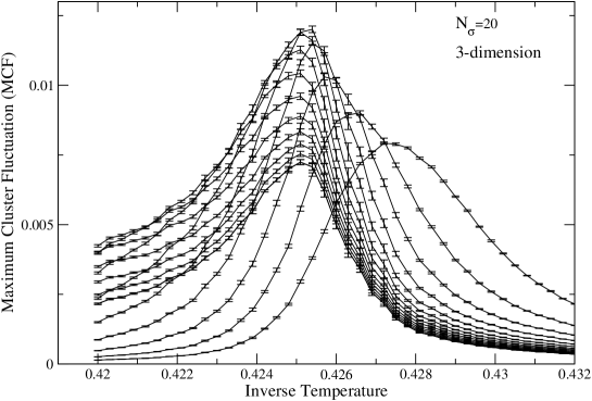
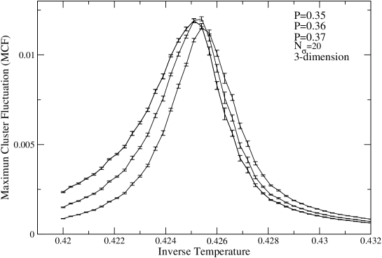
Figure 1:

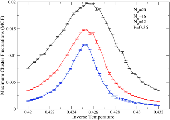
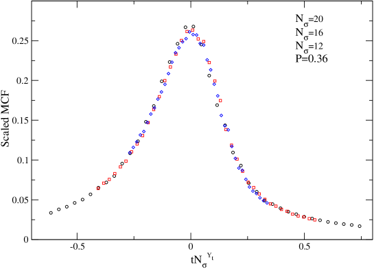
Figure 2:

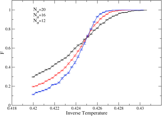
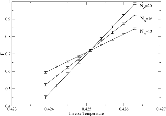
Figure 3:

References

- [1] A. M. Polyakov, Physics Letters B 72 (1978) 477 ; L. Susskind, Physical Review D 20 (1979) 2619 .
- [2] B. Svetitsky, L. Yaffe, Nuclear Physics B 210 [FS6] (1982) 423 ; L. Yaffe, B. Svetitsky, Physical Review D 26 (1982) 963; B. Svetitsky, Physics Reports 132 (1986) 1 .
- [3] J. Kertész, Physica A 161 (1989) 58 .
- [4] H. Satz, Nucl. Phys. A 642 (1998) 130 .
- [5] H. Satz, Nucl. Phys. A 681 (2001) 3.
- [6] P. W. Kasteleyn, C. M. Fortuin, Journal of the Physical Society of Japan 26 (Suppl.) (1969) 11 .
- [7] A. Coniglio, W. Klein, Journal of Physics A 13 (1980) 2775 .
- [8] S. Fortunato, F. Karsch, P. Petreczky, H. Satz, Phys. Lett. B502 (2001) 321
- [9] S. Fortunato, F. Karsch, P. Petreczky, H. Satz, Nucl. Phys. Proc. Suppl. 94 (2001) 398 .
- [10] S. Fortunato and H. Satz, Nucl. Phys. A 681 (2001) 466 .
- [11] S. Fortunato, H. Satz, Nucl. Phys. Proc. Suppl. 83 (2000) 452 .
- [12] P. Blanchard , S. Digal , S. Fortunato, D. Gandolfo, T. Mendes, H. Satz J.Phys. A 33 (2000) 8603 .
- [13] S. Fortunato, H. Satz, Nucl. Phys. B 598 (2001) 601 .
- [14] P. Bialas, P. Blanchard, S. Fortunato, D. Gandolfo, H. Satz, Nucl. Phys. B 583 (2000) 368 .
- [15] F. Green, F. Karsch, Nucl. Phys. B 238 (1984) 297 .
- [16] D. Stauffer, A. Aharony, Taylor & Francis, London 1994.
- [17] S. Demirtürk, Y. Gündüç, International Journal of Modern Physics C 12 (2001) 1361.
- [18] P.M.C. de Oliveira, Europhys. Lett. 20, (1992) 621.
- [19] P.M.C. de Oliveira, Physica A 205, (1994) 101.
- [20] J.M. de F. Neto, S.M. de Oliveira, and P.M.C. de Oliveira, Physica A 206, (1994) 463.
- [21] P.M.C. de Oliveira, S.M. de Oliveira, C.E. Cordeiro, and D. Stauffer, J. Stat. Phys. 80, (1995) 1433.
- [22] S. Demirtürk, N. Seferoglu, M. Aydın and Y. Gündüç, International Journal of Modern Physics C 12, (2001) 403.