A non-perturbative study of the action parameters for anisotropic-lattice quarks

Abstract

A quark action designed for highly anisotropic lattice simulations is discussed. The mass-dependence of the parameters in the action is studied and the results are presented. Applications of this action in studies of heavy quark quantities are described and results are presented from simulations at an anisotropy of six, for a range of quark masses from strange to bottom.

I Introduction

The anisotropic lattice has proved an invaluable tool for simulations of a variety of physical quantities. The precision calculation of the glueball spectrum was an early application of the approach Morningstar and Peardon (1999) and it was recognised that anisotropic actions may also be advantageous in heavy quark physics calculations Alford et al. (1997). Correlators of heavy particles such as glueballs and hadrons with a charm or bottom quark have a signal which decays rapidly. Monte Carlo estimates of these correlation functions can be noisy, making it difficult to resolve a plateau over a convincing range of lattice time steps. Increasing the number of timeslices for which the effective mass of a particle has reached a plateau solves this problem and also decreases the statistical error in the fitted mass. Since this value may be used as an input to determine many physical parameters this decrease is very beneficial.

Secondly, improved precision in effective mass fits means that momentum-dependent errors of ${\cal O}(ap)$ can be disentangled from other discretisation effects and larger particle momenta may be considered. This is particularly relevant for the determination of semileptonic decay form factors where the overlap of momentum regions accessible to experiments and lattice calculations is currently very small. Typically, experiments have more events with daughter particle momentum at or above 1 GeV. This is also the region where large momentum-dependent errors are expected in lattice calculations. The form factors of decays like $B\rightarrow\pi\ell\nu$ and $B\rightarrow K^{\ast}\gamma$ are inputs to determinations of CKM parameters so that increased precision in lattice calculations can lead to tighter constraints on the Standard Model. This has motivated a study of 2+2 anisotropic lattices where the temporal and one spatial direction are made fine and all momentum is injected along this fine spatial axis. Details of the progress to date in this work are in Refs. Burgio et al. (2003a) and Burgio et al. (2003b). The 2+2 formulation has also proved useful for a precision determination of the static interquark potential over large separations, which is described in Ref. Burgio et al. (2003a). In this paper we consider a 3+1 anisotropic action. The temporal lattice spacing, $a_{t}$ is made fine relative to the spatial spacing, $a_{s}$. The action is designed with simulations at large anisotropies in mind. To simulate a bottom quark with a relativistic action requires a lattice spacing of less than $0.04$ fm which is prohibitively expensive on an isotropic lattice where the simulation cost scales at least as ${\cal O}(a^{-4})$. The anisotropic lattice offers the possibility of relativistic heavy-quark physics using reasonably modest computing resources. In the rest frame of a hadron with a heavy constituent, the quark four-momentum is closely aligned with the temporal axis, allowing an anisotropic discretisation to represent accurately the Dirac operator on the quark field.

Implementing an anisotropic programme incurs a number of computational overheads not associated with the isotropic lattice. The ratio of scales, $\xi=a_{s}/a_{t}$ determined by studying a physical long-distance probe depends on bare parameters in the lattice action. While this dependence is straightforward to establish at the tree-level of perturbation theory, quantum corrections can occur at higher orders. In the quenched approximation on a 3+1 lattice this is not a serious additional cost as the tuning can be done post-hoc. More worringly, in Ref. Harada et al. (2001) it was pointed out that the choice of $\xi$ and its relation to the Wilson parameter, $r$ on anisotropic versions of the Sheikholeslami-Wohlert (SW) action could introduce ${\cal O}(a_{s}m_{q})$ errors. It is exactly errors of this type that the anisotropic action seeks to avoid and the appearance of these terms represents a serious tuning problem.

In this paper we use an action, specifically designed for highly anisotropic lattices ie. $\xi\geq 5$. By applying different improvement terms in the spatial and temporal directions the action is both doubler and ${\cal O}(a_{s}m_{q})$ error free. This opens up the possibility of simulating directly at the bottom quark mass using a relativistic action. In addition, in this feasibility study the speed of light was determined at $\approx$ 1% accuracy. This precision was governed by finite statistics and could certainly be improved upon.

The paper is organised as follows. The construction of the action is described in Section II. Section III compares this action with the sD34 action proposed in Ref. Hashimoto and Okamoto (2003) and details some analytic results. Results from a study of the dispersion relations and the mass-dependence of the speed of light are described in Section IV. Some preliminary results of this study have appeared in Ref. Foley et al. (2003). Our conclusions and a discussion of future work are contained in Section V.

II Designing highly anisotropic actions

We begin by considering a Wilson-type action with Symanzik improvement to remove discretisation errors. Full ${\cal O}(a)$-improvement requires a clover term and a field rotation, given by

$$\psi = [1-\frac{ra}{4}(/D-m)]\psi^{\prime},$$ (1)

$$\bar{\psi} = \bar{\psi^{\prime}}[1-\frac{ra}{4}(/D-m)],$$ (2)

where $a$ is the lattice spacing on an isotropic lattice and $r$ is the usual Wilson parameter. The rotation described by Eqs. (1) and (2) preserves locality and maintains a positive transfer matrix so that ghost states do not arise in a calculation of the free fermion propagator. However, in an anisotropic implementation of this action, when $a_{t}$ is made very small, these rotations may lead to the reappearance of doublers, an undesirable side-effect of the anisotropy.

We would like to maintain the useful properties of actions with nearest neighbour temporal interactions only. In particular, the positivity of the transfer matrix guarantees that effective masses approach a plateau from above. Therefore, to construct an action suitable for high anisotropies we begin by applying field rotations in the temporal direction only, rewriting Eqs. (1) and (2) as

$$\psi = [1-\frac{ra_{t}}{4}(\gamma_{0}D_{0}-m)]\psi^{\prime},$$ (3)

$$\bar{\psi} = \bar{\psi^{\prime}}[1-\frac{ra_{t}}{4}(\gamma_{0}D_{0}-m)].$$ (4)

This leads to a new action in which the temporal and spatial directions are treated differently. Having applied the rotations of Eqn. (2) the continuum action is given by

$$S^{\prime}=\bar{\psi^{\prime}}M_{r}\psi^{\prime}-\frac{ra_{t}}{2}\bar{\psi^{\prime}}\left(D_{0}^{2}-\frac{g}{2}\epsilon_{i}E_{i}\right)\psi^{\prime}.$$ (5)

where $M_{r}=\mu_{r}\gamma_{i}D_{i}+\gamma_{0}D_{0}+\mu_{r}m$ and $\mu_{r}=(1+\frac{1}{2}ra_{t}m)$. At the tree-level, the rotations described in Eqs. (3) and (4) do not generate a spatial clover term. As a result the ($\mathbf{\sigma\cdot B}$) term does not appear in Eq. (5). The chromoelectric field, $E_{i}$ is defined as

$$igE_{i}=[D_{i},D_{0}],$$ (6)

and $\epsilon_{i}\equiv\sigma_{i0}$ is given by $\epsilon_{i}=\displaystyle{\frac{1}{2i}}[\gamma_{i},\gamma_{0}]$.

The temporal doublers are removed by discretising the $D_{0}^{2}$ term in the usual way. However, with no spatial rotation the spatial doublers remain and must be treated separately. They are removed by adding a higher-order, irrelevant operator to the action. This was first suggested by Hamber and Wu in Ref. Hamber and Wu (1983). The simplest such operator is a spatial $D^{4}$ term which is added ad hoc to the Dirac operator giving an action,

$$S^{\prime}=\bar{\psi^{\prime}}M_{r}\psi^{\prime}-\frac{ra_{t}}{2}\bar{\psi^{\prime}}\left(D_{0}^{2}-\frac{g}{2}\epsilon_{i}E_{i}\right)\psi^{\prime}+sa_{s}^{3}\bar{\psi^{\prime}}\sum_{i}D^{4}_{i}\psi^{\prime}.$$ (7)

This approach has previously been discussed in detail in Ref. Peardon (2002). In this formulation, $s$ is a Wilson-like parameter which is chosen such that the doublers receive a sufficiently large mass. The discretisation of the action in Eq. (7) is now straightforward. Only the $\gamma_{i}D_{i}$ term requires an improved discretisation since the simplest discretisation would lead to ${\cal O}(a_{s}^{2})$ errors. For this case we write

$$\Delta_{imp}^{(1)}\phi(x) = \frac{1}{a}\left\{\frac{2}{3}\left[\phi(x+a)-\phi(x-a)\right]\right.$$ (8)

$$\left.-\frac{1}{12}\left[\phi(x+2a)-\phi(x-2a)\right]\right\}$$

and similarly the (unimproved) discretisations of $\partial$, $\partial^{2}$ and $\partial^{4}$ are

$$\Delta^{(1)}\phi(x) = \frac{1}{2a}\left\{\phi(x+a)-\phi(x-a)\right\},$$ (9)

$$\Delta^{(2)}\phi(x) = \frac{1}{a^{2}}\left\{\phi(x+a)+\phi(x-a)-2\phi\right\},$$ (10)

$$\Delta^{(4)}\phi(x) = \frac{1}{a^{4}}\left\{\left[\phi(x+2a)+\phi(x-2a)\right]\right.$$ (11)

$$- \left.4\left[\phi(x+a)-\phi(x-a)\right]+6\phi(x)\right\}.$$

The corresponding gauge covariant derivatives, $D$, $D^{2}$ and $D^{4}$ respectively are constructed by including link variables in the usual way. The chromoelectric field is discretised by a clover term with plaquettes in the three space-time planes only

$$gE_{i}=\frac{1}{\xi a_{t}^{2}}\frac{1}{u_{s}^{2}u_{t}^{2}}\frac{1}{8i}\left\{\Omega_{i}(x)-\Omega^{\dagger}_{i}(x)\right\},$$ (12)

with

$$\Omega_{i}(x) = U_{i}(x)U_{t}(x+\hat{\imath})U_{i}^{\dagger}(x+\hat{t})U_{t}^{\dagger}(x)$$

$$+ U_{t}(x)U_{i}^{\dagger}(x-\hat{\imath}+\hat{t})U_{t}^{\dagger}(x-\hat{\imath})U_{i}(x-\hat{\imath})$$

$$+ U_{i}^{\dagger}(x-\hat{\imath})U_{t}^{\dagger}(x-\hat{\imath}-\hat{t})U_{i}(x-\hat{\imath}-\hat{t})U_{t}(x-\hat{t})$$

$$+ U_{t}^{\dagger}(x-\hat{t})U_{i}(x-\hat{t})U_{t}(x+\hat{\imath}-\hat{t})U_{i}^{\dagger}(x).$$

$u_{s}$ and $u_{t}$ are the mean-link improvement parameters. $u_{s}$ is determined from the spatial plaquette and $u_{t}$ is set to unity. At the accuracy of the action constructed here no improvement is required. Finally, including the gauge fields and the mean-link improvement factors the lattice fermion matrix is given by,

$$M_{\rm ARIA}\psi(x) = \frac{1}{a_{t}}\left\{\left(\mu_{r}ma_{t}+\frac{18s}{\xi}+r+\frac{ra_{t}^{2}g}{4}\epsilon_{i}E_{i}\right)\psi(x)-\frac{1}{2u_{t}}\left[(r-\gamma_{0})U_{t}(x)\psi(x+\hat{t})+(r+\gamma_{0})U_{t}^{\dagger}(x-\hat{t})\psi(x-\hat{t})\right]\right.$$ (14)

$$\left.-\frac{1}{\xi_{q}}\sum_{i}\left[\frac{1}{u_{s}}(4s-\frac{2}{3}\mu_{r}\gamma_{i})U_{i}(x)\psi(x+\hat{\imath})+\frac{1}{u_{s}}(4s+\frac{2}{3}\mu_{r}\gamma_{i})U_{i}^{\dagger}(x-\hat{\imath})\psi(x-\hat{\imath})\right.\right.$$

$$\left.\left.-\frac{1}{u_{s}^{2}}(s-\frac{1}{12}\mu_{r}\gamma_{i})U_{i}(x)U_{i}(x+\hat{\imath})\psi(x+2\hat{\imath})-\frac{1}{u_{s}^{2}}(s+\frac{1}{12}\mu_{r}\gamma_{i})U_{i}^{\dagger}(x-\hat{\imath})U_{i}^{\dagger}(x-2\hat{\imath})\psi(x-2\hat{\imath})\right]\right\}.$$

At the tree-level, the fermion anisotropy $\xi_{q}$ is given by the ratio of scales, $\xi=a_{s}/a_{t}$. We call the action described here ARIA for Anisotropic, Rotated, Improved Action. It is classically improved to ${\cal O}(a_{t},a_{s}^{3})$.

III Heavy quarks with ARIA

The precision calculation of the glueball spectrum on coarse lattices Morningstar and Peardon (1999) suggests that heavy hadronic quantities would also benefit from the anisotropic formulation. The correlation functions for heavy-heavy and heavy-light mesons fall off rapidly with time and it can be difficult to isolate a convincing plateau over a reasonable number of timeslices. A lattice with fine temporal direction in principle solves this problem by providing a large number of timeslices over which the time-dependence can be resolved. Improved Wilson actions on anisotropic lattices have been used to study a range of heavy flavour physics including charmonium and bottomonium spectroscopy Okamoto et al. (2002); Liao and Manke (2002); Chen (2001), heavy-light and hybrid spectra Edwards et al. (2003); Matsufuru et al. (2003); Luo and Mei (2003); Harada et al. (2002) and also heavy-light semileptonic decays Shigemitsu et al. (2002).

In these calculations, currents are improved using rotations, which are applied identically in all four space-time directions and the Wilson parameter in the spatial direction is usually chosen to be either $r_{s}=1/\xi$ de Forcrand et al. (2000); Umeda et al. (2001) or $r_{s}=1=r_{t}$ Klassen (1998, 1999); Chen et al. (2001); Ali Khan et al. (2001). However, it was pointed out in Ref. Harada et al. (2001) that simulations with anisotropic Wilson-type actions may include ${\cal O}(a_{s}m_{q})$ effects. Naively, errors of this form are unexpected but they arise in products of the Wilson and mass terms in the action. In particular, the authors showed that the presence of these artefacts, which appear in radiative corrections, depends on the spatial Wilson parameter, $r_{s}$. The ${\cal O}(a_{s}m_{q})$-dependence potentially spoils the benefits of working on an anisotropic lattice, especially at large quark masses.

In Ref. Hashimoto and Okamoto (2003) a different approach was adopted. Since the unwanted ${\cal O}(a_{s}m_{Q})$-dependent terms arise from the spatial Wilson term the authors propose an anisotropic D234-type action Alford et al. (1997) may be more suitable. In this case a rotation term is applied in the temporal direction only, removing the temporal doublers. Spatial doublers are removed by adding an irrelevant, dimension-four term to the Dirac operator. The authors showed to one-loop order in perturbation theory, that this so-called “sD34” action does not suffer from ${\cal O}(a_{s}m_{q})$ terms. Comparing the ARIA action proposed in Section II and the sD34 action from Ref. Hashimoto and Okamoto (2003) we see that these are the same, up to ${\cal O}(a_{t})$ improvement.

The D234 quark action on an anisotropic lattice Alford et al. (1997) is be written

$$S_{D234}=a_{t}a_{s}^{3}\sum_{x}\bar{\psi}(x)M\psi(x),$$ (15)

and writing $M$ in the notation of Ref. Hashimoto and Okamoto (2003)

$$M = m_{0}+\sum_{\mu}\nu_{\mu}\gamma_{\mu}\nabla_{\mu}(1-b_{\mu}a_{\mu}^{2}\Delta_{\mu})-\frac{1}{2}a_{t}\left(\sum_{\mu}r\Delta_{\mu}\right.$$ (16)

$$\left.+\sum_{\mu<\nu}c_{\rm SW}^{\mu}\sigma_{\mu\nu}F_{\mu\nu}\right)+\sum_{\mu}\nu_{\mu}d_{\mu}a_{\mu}^{2}\Delta_{\mu}^{2}.$$

The sD34 action is a special case of this action in which the parameters have the following values

$$\begin{array}[]{lll}(\nu_{0},\nu_{i})=(1,\nu);&(b_{0},b_{i})=(0,\frac{1}{6});&(d_{0},d_{i})=(0,\frac{1}{8});\\ (r_{0},r_{i})=(r_{t},0);&(c_{\rm SW}^{0},c_{\rm SW}^{i})=(0,c_{\rm SW}).&\\ \end{array}$$ (17)

and $\nu=(1+\frac{1}{2}r_{t}a_{t}m_{0})$. Substituting in Eq. (16) gives

$$M_{\rm sD34} = m_{0}+\sum_{i}\nu\gamma_{i}\nabla_{i}\left(1-\frac{1}{6}a_{s}^{2}\Delta_{i}\right)+\gamma_{0}\nabla_{0}$$ (18)

$$-\frac{a_{t}}{2}\left(r\Delta_{0}+c_{\rm SW}^{t}\sigma_{i0}F_{i0}\right)+\frac{1}{8}a_{s}^{3}\sum_{i}\nu\Delta_{i}^{2},$$

which is the action we use in our simulations, up to ${\cal O}(a_{t})$ improvement. Reexpressing the fermion matrix in our notation,

$$M_{\rm ARIA} = \mu_{r}m_{0}+\sum_{i}\mu_{r}\gamma_{i}\nabla_{i}\left(1-\frac{1}{6}a_{s}^{2}\Delta_{i}\right)+\gamma_{0}\nabla_{0}$$ (19)

$$-\frac{a_{t}}{2}\left(r\Delta_{0}-\frac{rg}{2}\sigma_{i0}F_{i0}\right)+sa_{s}^{3}\sum_{i}\Delta_{i}^{2},$$

where $s=1/8$ and $\mu_{r}=\left(1+\frac{1}{2}r_{t}a_{t}m_{0}\right)$.

III.1 Analytic results for ARIA

In this section the energy-momentum behaviour of the ARIA action is calculated. We begin by presenting results for general $r$ and $s$. The free-quark dispersion relation is obtained by solving $\det\widetilde{M}_{\rm ARIA}=0$ in momentum space where $\widetilde{M}_{\rm ARIA}$ is the Fourier transform of $M_{\rm ARIA}$ in Eq. (14). The energy-momentum relation is

$$\cosh(Ea_{t}) = \frac{r^{2}+r\omega(p)}{r^{2}-1}\pm$$ (20)

$$\frac{\sqrt{(r+\omega(p))^{2}+(1-r^{2})(1+a^{2}_{t}\tilde{\mathbf{p}}^{2})}}{r^{2}-1},$$

where $\omega(p)$ and $\tilde{\mathbf{p}}$ are defined as

$$\omega(p) = a_{t}\mu_{r}m_{0}+a_{t}s\sum_{i}a^{3}_{s}\hat{p}^{4}_{i},$$ (21)

$$\tilde{\mathbf{p}} = \mu_{r}\bar{p}_{i}(1+\frac{1}{6}a^{2}_{s}\hat{p}^{2}_{i}),$$ (22)

with $\bar{p}_{i}=\displaystyle{\frac{1}{a_{s}}}\sin(a_{s}p_{i})$ and $\hat{p}_{i}=\displaystyle{\frac{2}{a_{s}}}\sin(a_{s}p_{i}/2)$. Expanding the physical solution in powers of spatial momentum yields

$$E^{2}(\mathbf{p})=M_{1}^{2}+\frac{M_{1}}{M_{2}}\mathbf{p}^{2}+O(\mathbf{p}^{4}),$$ (23)

where $M_{1}$ is the rest mass, given by

$$M_{1}=\frac{1}{a_{t}}\cosh^{-1}\left(\frac{r^{2}+\mu_{r}m_{0}ra_{t}-\sqrt{1+2\mu_{r}m_{0}ra_{t}+m_{0}^{2}\mu^{2}_{r}a^{2}_{t}}}{r^{2}-1}\right).$$ (24)

The kinetic mass, $M_{2}$ is given by

$$\frac{1}{M_{2}}=\frac{\mu^{2}_{r}a_{t}}{\sqrt{1+2\mu_{r}m_{0}ra_{t}+m_{0}^{2}\mu^{2}_{r}a^{2}_{t}}}\left[\left(\frac{r^{2}+\mu_{r}m_{0}ra_{t}-\sqrt{1+2\mu_{r}m_{0}ra_{t}+m_{0}^{2}\mu^{2}_{r}a^{2}_{t}}}{r^{2}-1}\right)^{2}-1\right]^{-\frac{1}{2}}.$$ (25)

Eqs. (24) and (25) indicate that at the tree-level $M_{1}$ and $M_{2}$ do not depend on ${\cal O}(a_{s}m_{q})$ terms or on the ratio of scales, $\xi$.

To compare these expressions with the results of other studies, the particular choice $r=1$ was considered. In this case the lattice ghost (the unphysical solution of Eq. (20)) disappears and the dispersion relation is given by

$$4\sinh^{2}\left(\frac{Ea_{t}}{2}\right)=\frac{a^{2}_{t}\tilde{\mathbf{p}}^{2}+\omega^{2}(p)}{1+\omega(p)},$$ (26)

with

$$M_{1} = \frac{1}{a_{t}}\log(1+\mu_{r}m_{0}a_{t}),$$ (27)

$$\frac{1}{2M_{2}} = \frac{\mu_{r}}{m_{0}(2+\mu_{r}m_{0}a_{t})}.$$ (28)

where now $\mu_{r}=(1+\frac{1}{2}a_{t}m_{0})$. These expressions are consistent with those obtained in Ref. Hashimoto and Okamoto (2003) for the sD34 action and in Ref. El-Khadra et al. (1997) for the Fermilab action on an isotropic lattice.

The free-quark dispersion relations for massless and massive quarks are shown in Figure 1. The anisotropy parameter, $\xi$ is six for both cases.

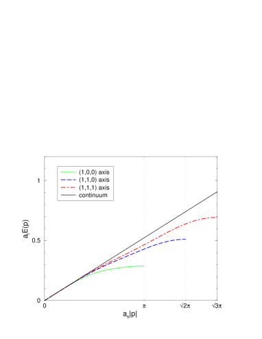
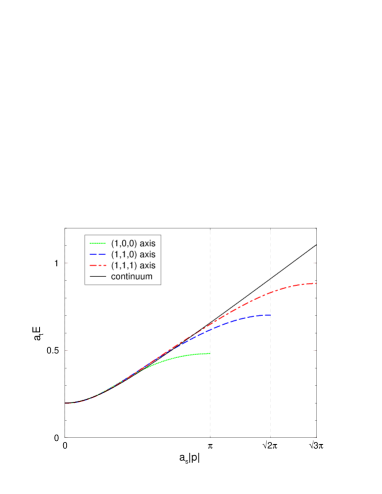
Figure 1: The dispersion relations given by Eq. 20 with $\xi=6$, $r=1$ and $s=1/8$. The top figure is the massless case while the bottom plot shows the massive case, with $a_{t}m_{q}=0.2$.

In analogy to the traditional Wilson $r$-parameter, the parameter $s$ in this action can in principle take any positive value. We chose $s=1/8$ by eye, demanding that the energy-momentum relations do not have negative slope for $a_{s}|p|<\pi$. Since $s$ parameterises a term which removes the spatial doublers and is irrelevant in the continuum limit precise tuning is not required.

IV Results

In this exploratory study the temporal rotations have been omitted which leads to an ${\cal O}(a_{t})$ classical discretisation error. However, since $a_{t}$ is small in these simulations, $a_{t}\sim 0.04$ fm, the effects should be under control at least when $a_{t}m_{q}<1$. Discarding temporal rotations means the action has no clover term and in addition we have set $\mu_{r}=1$. It is planned to include correction terms to remove ${\cal O}(a_{t})$ errors in future work.

The ratio of scales is changed in a simulation by quantum corrections. Therefore the action parameter must be adjusted so that the ratio of scales measured from a physical quantity is correct. In a quenched simulation the parameters $\xi_{g}$ and $\xi_{q}$ in the gauge and quark actions may be independently tuned to the target anisotropy, using different physical probes. This is not the case for unquenched simulations where the anisotropy in the gauge and quark actions must be tuned simultaneously Peardon (2002).

For this study an ensemble of quenched gauge configurations for which $\xi_{g}$ had already been tuned was used. In this case the tuning criterion was that $\xi=6$ when measured from the static interquark potential in different directions on the lattice. The parameter $\xi_{q}$ in the fermion action must now be tuned such that its value determined from the energy momentum dispersion relation is six. At this point we introduce some terminology which makes clear the difference between $\xi_{q}$, which is a parameter in the action, and the slope of the dispersion relation which is a physical observable – usually called the speed of light, $c$. The target anisotropy is six. $\xi_{q}$ is tuned so that the speed of light (determined from the slope of the dispersion relation) is unity.

The anisotropic action offers the possibility of precision studies of a range of phenomenologically interesting heavy quark quantities in the $D$, $B$, $J/\psi$ and $\Upsilon$ sectors. For this reason it is important to understand the dependence of $\xi_{q}$ on the heavy quark mass used in simulations. In particular, a contribution of ${\cal O}(a_{s}m_{q})$ to the renormalised anisotropy would spoil this tuning for charm and bottom quark masses. The main result in this section is a study of the mass-dependence of the speed of light at fixed anisotropy.

IV.1 Simulation parameters

The gauge action used in this simulation is a two-plaquette improved action designed for precision glueball simulations on anisotropic lattices. A description is given in Ref. Morningstar and Peardon (2000). The construction of the fermion action is described in detail in Section II. Details of the simulation and parameter values are summarised in Table 1.

# gauge configurations	100
Volume	$10^{3}\times 120$
$a_{s}$	0.21fm
$a_{s}/r_{0}$	0.4332(11)
$\xi=a_{s}/a_{t}$	6
$a_{t}m_{q}$	-0.04,0.1,0.2,0.3,0.4,0.5,1.0,1.5

Table 1: Details of the simulation.

A broad range of quark masses was investigated, from $a_{t}m_{q}=-0.04$ which is close to the strange quark on these lattices to heavy quarks with $a_{t}m_{q}=1.0$ and $1.5$. Both degenerate and nondegenerate combinations are considered. The nondegenerate combination is made with the lightest quark and each of the heavier quarks. Note that $a_{t}m_{q}=-0.04$ corresponds to a positive quark mass since Wilson-type actions have an additive mass renormalisation. We accumulated data at spatial momenta (0,0,0), (1,0,0), (1,1,0) and (1,1,1), in units of $2\pi/a_{s}L$, averaging over equivalent momenta.

It is worth noting that all the gauge configurations and quark propagators used in this study were generated on Pentium IV workstations. Generating the lightest quark propagators (close to the strange quark mass) required approximately one week on a single processor. At this quark mass no exceptional configurations were seen.

IV.2 Effective masses

The success of anisotropic lattice methods is predominantly due to the increased resolution in the temporal direction. The fineness of the lattice in this direction is particularly useful when determining heavy mass quantities whose signal to noise ratio decreases rapidly. The increase in resolution also leads to reduced statistical errors in effective masses since fits can be made to longer time ranges than is usually possible with an isotropic lattice. For the same reason, the fitted values tend to be less sensitive to fluctuations of one or two points in the chosen fit range.

In this study the effective masses were determined using single cosh fits with a $\chi^{2}$ minimization algorithm. The signal to noise ratio was enhanced by using four sources, distributed across the lattice at timeslices 0, 30, 60 and 90. The average of these results was used in the effective mass fits. The statistical errors shown are calculated from 1000 bootstrap samples in each fit. Figure 2 shows four effective mass plots. The first plot is the pseudoscalar meson with degenerate quarks at the lightest mass for zero momentum and for momentum of $(1,1,1)$ in lattice units, $2\pi/a_{s}L$. The second plot is the analogous case for the degenerate combination of quarks with $a_{t}m_{q}=1.0$. In all cases a clear plateau, over a large number of timeslices is observed. The fits to effective masses of the non-degenerate mesons are equally good and in all cases the fit range is ten or more timeslices with a $\chi^{2}$ per degree of freedom ($\chi^{2}/N_{df}$) $\sim 1$.

Figure 2: Pseudoscalar meson effective mass plots. The two plots indicate that very good fits can be made for a wide range of quark masses and momenta. The top plot shows the effective mass of the lightest meson made from a degenerate combination of quarks with $a_{t}m_{q}=-0.04$ for zero momentum and for three units of momentum in lattice units. The second plot is the analogous case for $a_{t}m_{q}=1.0$.

In Figure 3 the equivalent results for vector mesons are presented. Once again, the lightest and heaviest degenerate combinations of quark masses considered are shown and very good fits are possible in both cases.

Figure 3: Vector meson effective mass plots. As in the pseudoscalar case shown in Figure 2, good fits are achieved over a large number of timeslices for all the quark masses considered in this study. The top plot shows the lightest degenerate vector while the bottom plot shows the same result for $a_{t}m_{q}=1.0$.

IV.3 The renormalised anisotropy

The slope of the energy momentum dispersion relation is determined nonperturbatively and compared to the target anisotropy, $\xi=6$. We are interested in both the precision of the determination and the deviation of the speed of light from unity. The wide range of quark masses used in this simulation ($a_{t}m_{q}=-0.04$ to $a_{t}m_{q}=1.5$) allow us to study the mass-dependence of the renormalisation. We also examine the difference between the anisotropy determined from particles with degenerate and non-degenerate quark content.

To begin, the dispersion relation was determined for a pseudoscalar meson made from the lightest quarks in this simulation, $a_{t}m_{q}=-0.04$ and with an input anisotropy, $\xi_{q}=6.0$. The value of $c$ determined from the dispersion relation was used to determine the tuned value of the anisotropy, $\xi_{q}=6.17$ and the calculation repeated. The resulting dispersion relation is shown in Figure 4. The subsequent value of $c$ determined from this data is $1.02\pm 0.01$.

Figure 4: The energy-momentum for the lightest degenerate meson in this simulation. The bare quark mass is $a_{t}m_{q}=-0.04$.

This value of $\xi_{q}=6.17$ was then used in simulations for a range of quark masses, $0.1\leq a_{t}m_{q}\leq 1.5$. A representative sample of the energy-momentum dispersion relations for this range of quark masses and particles is shown in Figure 5.

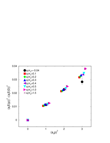
Figure 5: The energy momentum dispersion relation for the pseudoscalar meson at all the masses simulated. The lightest point, $a_{t}m_{q}=-0.04$ is close to the strange quark while the heaviest mass is close to the bottom mass. The points have been shifted about their momentum value to make the plot easier to read.

The plot shows very good linear dispersive behaviour. This relativistic dispersion relation persists for both degenerate and non-degenerate quark combinations in pseudoscalar and vector particles at all masses.

The mass-dependence of the speed of light is given by the difference in the slopes for the different masses. Figure 5 shows that this dependence is mild. The lightest mass, close to the strange quark mass, is the noisiest and the statistical errors increase with increasing momentum, as expected. It should be noted that the quark propagators used in this study are generated with point sources and the use of smearing techniques is expected to improve the signal for this and lighter quark masses. In addition the advantages of stout link gauge backgrounds Morningstar and Peardon (2004) will be investigated in further studies.

In Tables 2 and  3 we show the speed of light determined from the slope of the dispersion relation for each mass in the simulation. The $\chi^{2}/N_{d.f.}$ for these fits also is shown. Results for both pseudoscalar and vector mesons are given and the ground state masses extracted in the fitting procedure described in Section IV.2 are listed.

	Pseudoscalar			Vector
$a_{t}m_{q}$	$a_{t}M_{PS}$	$c$	$\chi^{2}/N_{df}$	$a_{t}M_{V}$	$c$	$\chi^{2}/N_{df}$
-0.04	$0.1045^{+5}_{-5}$	$1.02^{+1}_{-1}$	$6.3/2$	$0.161^{+2}_{-2}$	$0.97^{+2}_{-2}$	$0.66/2$
0.10	$0.3831^{+4}_{-4}$	$0.983^{+6}_{-7}$	$2.8/2$	$0.3934^{+4}_{-4}$	$0.982^{+8}_{-8}$	$2.1/2$
0.20	$0.5418^{+3}_{-4}$	$0.995^{+7}_{-7}$	$0.33/2$	$0.5472^{+4}_{-4}$	$0.990^{+8}_{-8}$	$2.1/2$
0.30	$0.6887^{+4}_{-4}$	$1.010^{+8}_{-7}$	$2.4/2$	$0.6924^{+4}_{-4}$	$0.997^{+9}_{-9}$	$4.5/2$
0.40	$0.8269^{+4}_{-4}$	$1.022^{+5}_{-5}$	$0.65/2$	$0.8294^{+4}_{-4}$	$1.011^{+5}_{-5}$	$2.3/2$
0.50	$0.9569^{+4}_{-4}$	$1.035^{+5}_{-5}$	$1.3/2$	$0.9587^{+4}_{-4}$	$1.025^{+5}_{-5}$	$1.6/2$
1.00	$1.5086^{+3}_{-3}$	$1.069^{+5}_{-5}$	$1.3/2$	$1.5092^{+3}_{-3}$	$1.072^{+5}_{-5}$	$1.2/2$
1.50	$1.9428^{+3}_{-3}$	$1.075^{+5}_{-5}$	$0.081/2$	$1.9431^{+3}_{-4}$	$1.072^{+5}_{-5}$	$0.058/2$

Table 2: The ground state pseudoscalar and vector masses with degenerate quarks. The speed of light determined from the dispersion relation for each quark mass is shown with the associated $\chi^{2}/N_{d.f.}$. The errors in all cases are statistical only. The parameter, $\xi_{q}$ is fixed in these simulations to $6.17$, its value determined from the dispersion relation of the lightest degenerate pseudoscalar meson.

	Pseudoscalar			Vector
$a_{t}m_{q}$	$a_{t}M_{PS}$	$c$	$\chi^{2}/N_{df}$	$a_{t}M_{V}$	$c$	$\chi^{2}/N_{df}$
0.1	$0.2610^{+6}_{-6}$	$0.98^{+1}_{-1}$	$0.23/2$	$0.2802^{+8}_{-8}$	$0.98^{+2}_{-2}$	$0.19/2$
0.2	$0.3466^{+6}_{-6}$	$1.01^{+2}_{-2}$	$0.56/2$	$0.3601^{+8}_{-8}$	$0.99^{+2}_{-2}$	$0.64/2$
0.3	$0.4254^{+7}_{-7}$	$1.02^{+2}_{-2}$	$2/2$	$0.4351^{+8}_{-8}$	$1.00^{+2}_{-2}$	$0.45/2$
0.4	$0.4987^{+7}_{-7}$	$1.01^{+2}_{-2}$	$1.5/2$	$0.5056^{+8}_{-9}$	$0.99^{+2}_{-2}$	$1.4/2$
0.5	$0.5668^{+8}_{-8}$	$1.02^{+2}_{-2}$	$1.7/2$	$0.5720^{+9}_{-9}$	$1.00^{+2}_{-2}$	$1.6/2$
1.0	$0.8521^{+10}_{-10}$	$1.00^{+2}_{-2}$	$2.6/2$	$0.854^{+1}_{-1}$	$1.02^{+3}_{-3}$	$0.62/2$
1.5	$1.074^{+1}_{-1}$	$1.02^{+3}_{-3}$	$2.1/2$	$1.075^{+1}_{-1}$	$1.01^{+3}_{-4}$	$1.8/2$

Table 3: The ground state masses of non-degenerate combinations of quark masses. In each case the quark mass given is combined with the lightest mass in our simulations, $a_{t}m_{q}=-0.04$. As in Table 2 the pseudoscalar and vector meson states are shown with the speed of light and the associated $\chi^{2}/N_{d.f.}$. Once again all errors are statistical only and $\xi_{q}=6.17$.

The dependence of $c$ on the quark mass in the simulation is shown in Figures 6 and 7. The plots show the speed of light as a function of the meson mass in units of $a_{t}$ for both pseudoscalars and vectors.

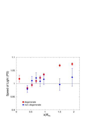
Figure 6: The mass-dependence of the speed of light determined from the pseudoscalar (PS) dispersion relations for fixed $\xi_{q}=6.17$. The plot shows mesons with both degenerate and non-degenerate quark mass combinations plotted as a function of the degenerate meson mass, in units of the temporal lattice spacing.

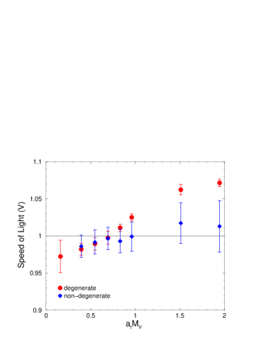
Figure 7: The mass-dependence of the speed of light determined from the vector (V) dispersion relations with $\xi_{q}=6.17$. Both degenerate and non-degenerate mass combinations are shown, plotted as a function of the degenerate vector mass as in Figure 6.

It is important to remember that the anisotropy was tuned only once at the lightest pseudoscalar particle. The plots show good agreement between determinations of $c$ from degenerate and non-degenerate particles up to $a_{t}m_{q}\sim 0.5$, corresponding to $a_{t}M_{PS}=0.957(5)$ in Figure 6. The charm quark mass on this lattice is close to $a_{t}m_{q}=0.2$, implying that charm physics is both computationally feasible and requires little parameter tuning at an anisotropy of six. Figures 6 and 7 also show some quark mass dependence for degenerate mesons with $a_{t}m_{q}\geq 0.5$. They also indicate that the agreement between the degenerate and non-degenerate meson physics decreases for $a_{t}m_{q}\geq 0.5$. This is not unexpected since degenerate mesons with two heavy quarks (charmonium and bottomonium) have a small Bohr radius and can suffer large discretistation effects. The non-degenerate mesons ($D$ and $B$ mesons) do not have such a problem.

We have investigated this dependence by varying the parameter $\xi_{q}$ in the quark action and repeating the simulations described above, for the heavy quark mass $a_{t}m_{q}=1.0$. The dependence of the speed of light, determined from the dispersion relation, on the input anisotropy is shown in Figure 8.

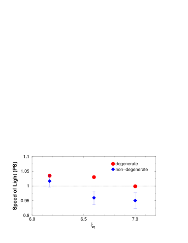
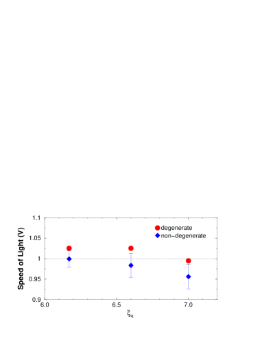
Figure 8: The speed of light as measured from the dispersion relation as a function of the parameter, $\xi_{q}$ in the action. The first plot shows the result for the pseudoscalar (PS) meson, for both degenerate and non-degenerate combinations. The second plot is the analogous result for the vector (V) mesons. In both cases the quark mass is fixed at $a_{t}m_{q}=1.0$.

The value of $c$ determined from the degenerate meson moves closer to its target value of unity and $c$ determined from the non-degenerate physics moves away from this value. It is also interesting to note the agreement between determinations of $c$ from pseudoscalar and vector particles. The tuning, described above at $a_{t}m_{q}=-0.04$ was carried out for pseudoscalars and it is reassuring that although the vector particles have larger statistical errors they nevertheless yield a consistent picture for the mass dependence of the speed of light.

V Discussion and Conclusions

In this paper we have explored the viability of anisotropic actions for heavy quark physics. An action suitable for simulations at large anisotropies and which has no ${\cal O}(a_{s}m_{q})$ errors is described. One of the main disadvantages of using anisotropic actions is the extra parameter tuning required to recover Lorentz invariance. In particular, if the ratio of scales $\xi$ is sensitive to the quark mass in the simulation then a parameter tuning may be required for each mass. We have measured the speed of light for a range of quark masses having fixed the ratio of scales at the strange quark, $a_{t}m_{q}=-0.04$. Only slight mass dependence (for the degenerate mesons) is found up, to $a_{t}m_{q}=0.5$ which is heavier than the charm quark on these lattices. This implies that one measurement of the speed of light is all that is required for simulations over a large range of masses, at the percent-level of simulation. The simulations were repeated for mesons with non-degenerate quarks, using a value of $\xi$ tuned from the degenerate meson spectrum. The results are in excellent agreement up to $a_{t}m_{q}=0.5$. Since the charm quark on this lattice is approximately $a_{t}m_{q}=0.2$ this work indicates that both heavy-heavy (degenerate) and heavy-light (non-degenerate) charm physics can be easily reached using an appropriately improved anisotropic action.

The results also show that heavy-light as well as heavy-heavy physics can be reliably simulated after a single tuning of $\xi_{q}$. The determination of $c$ can be interpreted as a measure of the ratio $M_{1}/M_{2}$ in Eq. (23). The agreement of $M_{1}$ and $M_{2}$ for both heavy-heavy and heavy-light systems can in turn be interpreted as an absence, in this quark action, of the anomaly first discussed in Ref. Collins et al. (1996). This anomaly was explained in Ref. Kronfeld (1997) where it was pointed out that for a sufficiently accurate lattice action (${\cal O}(v^{4})$ in NRQCD) the discrepancies in binding energies $\delta B=B_{2}-B_{1}$ vanishes and $I=(2\delta B_{\bar{Q}q}-(\delta B_{\bar{Q}Q}+\delta B_{\bar{q}q}))/2M_{2\bar{Q}q}=0$ as expected. The action described in this study has this property.

This study has been carried out in the quenched approximation which is a useful laboratory in which to study mass-dependent and tuning issues at relatively low computational cost. We are currently developing algorithms for dynamical simulations with anisotropic lattices which we plan to use in a study of heavy-flavour physics.