Spatially improved operators for excited hadrons on the lattice
Abstract
We present a new approach for determining spatially optimized operators that can be used for lattice spectroscopy of excited hadrons. Jacobi smeared quark sources with different widths are combined to construct hadron operators with different spatial wave functions. We use the variational method to determine those linear combinations of operators that have optimal overlap with ground and excited states. The details of the new approach are discussed and we demonstrate the power of the method using examples from quenched baryon and meson spectroscopy. In particular we study the Roper state and and discuss some physical implications of our tests.
pacs:
PACS: 11.15.HaI Introduction
Ground state spectroscopy on the lattice is by now a well understood physical problem and impressive agreement with experiment has been achieved. The lattice study of excited states is not so far advanced and for many systems even the correct level ordering of the states has not yet been observed. A prominent example for such a system is the nucleon and its excited states. In particular the first excited positive parity nucleon, the so-called Roper state, has seen a lot of attention from the lattice community during the last two years oldcalcs - broemmeletal . Revealing the true nature of the Roper state with non-perturbative methods is an important task.
In a lattice calculation the masses of excited states show up in the subleading exponentials of Euclidean two point functions. A direct fit of a single Euclidean correlator is cumbersome since the signal is strongly dominated by the ground state. Also with methods such as constrained fits constrainedfits or the maximum entropy method maximumentropy one still needs very high statistics for reliable results.
An alternative method is the computation of not only the correlator of a single operator, but the calculation of a full matrix containing all cross correlations of a set of several operators with the correct quantum numbers variation . In this so-called variational method the correlation matrix is then diagonalized and one can show that each eigenmode is dominated by a different physical state (for a properly chosen set of basis operators). After normalization at distance 0, for the largest eigenvalue gives the Euclidean correlator of the ground state, the second-largest eigenvalue corresponds to the first excited state, et cetera.
The success of the variational method depends strongly on the choice of the basis operators. They need to be linearly independent and should give rise to a large overlap with the physical states. A physical hadron state has several characteristics, in particular a specific Dirac structure and its spatial wave function. Therefore it is advantageous to optimize the spatial properties of the interpolating operators. An example for this fact is the mentioned Roper state where the variational method based on nucleon operators that differ only in their diquark content but have the same spatial wave function did not lead to success broemmeletal . It can be argued that a node in the radial wave function is necessary to capture reliably the Roper state or other radially excited hadrons.
In lattice calculations it is important to devise an efficient way of implementing a spatial wave function at low numerical cost. When the quark wave function extends over several lattice sites, a naive approach would require the inversion of the Dirac operator on point sources located at all possible quark positions (see wavefunction for a discussion of such wave functions). Creating a wave function for quarks in this way quickly becomes numerically expensive. For improving the ground state wave function an effective technique, so-called Jacobi smearing, has been shown to give good results jacobi . Here, a point-like quark source is smeared to a shape similar to a Gaussian, i.e. the origin of the source is connected to neighboring lattice sites within a time slice by gauge transporters. Such a source increases the overlap of the physical hadron states with the lattice operators used to create these states and considerably reduces the fluctuations of hadron propagators.
In this article we demonstrate that combining Jacobi smeared quark sources with different widths in the variational method provides a powerful tool for the analysis of excited hadron states. After presenting the outlined ideas in detail we apply our method to quenched baryon and meson spectroscopy. The excited nucleon system as well as excited mesons are analyzed (for recent lattice studies of excited mesons see mesons ). We find good effective mass plateaus for the first and partly the second radially excited states. The propagators can then be fitted using standard techniques. Different physical ramifications and implications of our findings are briefly discussed.
II The method
Let us begin the presentation of our method with a brief recapitulation of Jacobi smearing of quark sources. Since a complete quark propagator (the inverse of the lattice Dirac operator ) is a far too large object to be stored completely in the computer, one has to work with the propagator evaluated on some source . The source is placed at timeslice of the lattice. It is labeled by a Dirac index and a color index . One then computes ( and are summed over)
| (1) |
When one chooses a point-like source at the spatial origin , i.e. with
| (2) |
the resulting vector is the quark propagator from the origin to all lattice points. These quark propagators can then be combined to form hadron propagators.
Choosing a point-like quark source has, however, the big disadvantage of a poor overlap with the true wave function. After all, for the lattice spacings which are appropriate, quarks are not expected to be located at a single point inside the hadron and the overlap of the point-like wave function with the true physical wave function is small. The situation can be improved, e.g. by Jacobi smearing. One acts with a smearing operator on the point-like source to obtain the smeared source :
| (3) | |||||
The operator is simply the spatial hopping part of the Wilson term at timeslice 0. Note that , and thus , is trivial in Dirac space and acts only on the color indices (in our notation we suppress the color indices of , and of the gauge transporters ).
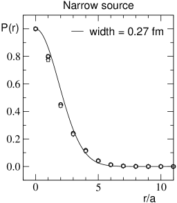
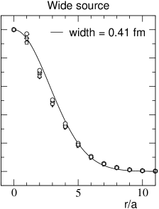
The Jacobi smearing outlined in Eq. (3) has two free parameters: The number of smearing steps and the positive real parameter . These two parameters can be used to adjust the profile of the source. In order to study the profile of the smeared source we define
| (4) |
Since the smearing is trivial in Dirac space the profile function is independent of the Dirac label which appears in the source . The profile function can, however, depend on the color label , but as we will demonstrate below this dependence is small. The delta function on the right hand side is implemented by binning the discrete values of on the lattice. We stress that is not a gauge invariant object, but only an auxiliary quantity to visualize the source. Certainly it is easy to construct a profile function which is a color singlet, but since we are interested in visualizing the sources individually for all , we use the form Eq. (4).
In this article we work with two different sources, a narrow source and a wide source with parameters given by
| (5) |
In Fig. 1 we show the profile functions for these two sources. They were normalized such that . For two different gauge configurations (, Lüscher-Weisz gauge action, , lattice spacing fm) we superimpose the values for for all three possible color indices of the original point source, i.e. for . It is obvious from the plots that the different color components of the point source lead to very similar profiles for the smeared source. Also when comparing different configurations, the relative fluctuations are small. The smearing parameters and were chosen such that the profiles approximate Gaussian distributions with widths of fm for the narrow source and fm for the wide source. These Gaussians are displayed as curves in Fig. 1.
We remark that the parameters were chosen such that simple linear combinations of the narrow and wide profile approximate the first and second radial wave functions of the spherical harmonic oscillator: The coefficients approximate a Gaussian with a width of fm, while the combination approximates the corresponding excited radial wave function with one node. Thus, the two sources we include allow the system to build up radial wave functions with and without a node.
The final form of the wave function is, however, not put in by hand, but is determined by the system through the variational method variation . In this approach one does not calculate a single correlator, but instead a complete correlation matrix of operators that create from the vacuum the state which one wants to analyze. One calculates all cross correlations
| (6) |
In Hilbert space this correlation matrix has the representation (for infinite temporal extent)
| (7) |
where the sum runs over all physical states and the corresponding energies are denoted as . The eigenvalues of the correlation matrix can be shown to behave as
| (8) |
where is the distance of to nearby energy levels. A modification of the method is the analysis of the generalized eigenvalue problem
| (9) |
which can be rewritten to a standard eigenvalue problem by bringing to the left hand side of Eq. (9), e.g. in the form of multiplied from the left. The normalization at some slice is expected to improve the signal by suppressing the contributions of higher excited states. We will explore the freedom of such a normalization in our analysis.
The sources we use for the correlation matrix are constructed from the narrow and wide quark sources we prepared. This is best explained in an example: An operator which creates the -meson is given by . Both the and the quark can either have a narrow () or a wide () quark source. This gives the four possible combinations , where the first entry refers to the smearing of the quark and the second entry is for the quark. Thus, we can use a basis of the four operators
| (10) |
for building up the correlation matrix . We remark that the different operators also have to be used at the sink end (timeslice ). This can be implemented by applying the smearing operator with the two sets of smearing parameters Eq. (5) at the sink end of the quark propagator.
Before we put our method to a test in the nucleon and meson systems let us briefly summarize some technical details. For our quenched calculation we use the chirally improved Dirac operator chirimp . It is an approximation of a solution of the Ginsparg Wilson equation GiWi82 which governs chiral symmetry on the lattice. The chirally improved Dirac operator is well tested in quenched ground state spectroscopy bgr where pion masses down to 250 MeV can be reached at a considerably smaller numerical cost than needed for exact Ginsparg Wilson fermions. For ground states the chirally improved action shows very good scaling behavior.
The gauge configurations we use for testing our method were generated on a lattice with the Lüscher-Weisz action Luweact . The inverse gauge coupling is , giving rise to a lattice spacing of fm as determined from the Sommer parameter in scale . The statistics of our ensemble is 100 configurations. We use 10 different quark masses ranging from to .
III Example A: Excited nucleons
The first example where we put our new method to a test is the spectroscopy of excited nucleons. Spectroscopy of the lowest positive and negative parity states is a key to understanding the physics of the nucleon. From a lattice perspective the nucleon system still holds a few unresolved puzzles and new methods will help to obtain a more complete picture.
It has long been noted that the observed ordering of the lowest positive, , and negative parity excitations of the nucleon, is ’unnatural’. Indeed, a physical picture based on linear confinement, Coulomb and color-magnetic terms, always arranges the first radial excitation above the first orbital excitation, i.e. the excited states have alternating parities. This outcome is in contrast to the observed nucleon masses, where the first radial excitation, , is well below the first orbital one, . This has prompted speculations that perhaps the Roper resonance is not a three quark state, but a collective excitation of the bag surface BROWN , a gluonic state CARBURKISS , a coupled channel effect KREWALD , a resonance in the pion - skyrmion system KARCOH , and most recently - a pentaquark state with a scalar diquark - scalar diquark - antiquark structure JW .
On the other hand, we have to expect that close to the chiral limit effects of the spontaneous breaking of chiral symmetry should be important. It has been suggested in GR that in the low-lying baryons the residual interaction between the valence constituent quarks mediated by the Goldstone boson field should be of vital importance. Such an interaction is of the flavor- and spin-exchange nature, contrary to the perturbative QCD degrees of freedom, and very naturally resolves the puzzle of low-lying baryon spectroscopy in the u,d,s sector.
If chiral symmetry breaking is important for the Roper state, we expect that the ordering of the lowest excitations of baryons should change as a function of the quark mass. Baryons made of heavy quarks, where chiral effects do not play a role, should show a radial excitation above the orbital excitation, while for smaller quark masses we expect a level reordering as seen in the nucleon system. At intermediate quark masses a level crossing of the radial and orbital excitations should take place. Hence, studying the evolution of the baryon spectrum versus the current quark mass allows one to clarify the physical picture. This can be done within the lattice approach where masses of quarks are external parameters which can be freely varied. In particular with the newly developed fermion actions based on the Ginsparg-Wilson equation the region of small quark masses also becomes accessible.
Previous attempts to study these issues on the lattice oldcalcs - broemmeletal have mainly used the two interpolating fields, and ,
| (11) | |||||
| (12) |
Here is the charge conjugation matrix and are the color indices. For the Dirac indices we use matrix notation. While the coupling of the operator to both the nucleon and the lowest negative parity state has been reliably established, the operator couples neither to the nucleon, nor to the Roper state. For a detailed study of this issue and for an interpretation of this fact see broemmeletal . Hence a remaining possibility to see the Roper state is to use and try to separate the strong signal of the ground state (the nucleon) from the weak signal of the radial excited state (the Roper state, if indeed the Roper state is a 3-quark state) at small Euclidean time. This strategy has been followed in Refs. dongetal and sasaki where in the former case a multi-exponential fit of the diagonal correlator has been performed (using constrained curve fitting constrainedfits ), while in the latter the maximum entropy method maximumentropy has been used. Both papers report the observation of the Roper resonance and level crossing towards the chiral limit. However, the two papers contradict each other on the value of the pion mass where this level switching takes place (300-400 MeV versus 600 Mev). Further improvement of the lattice technology is necessary to deepen the understanding of the nucleon system from the lattice.
Both the open physical and technical questions of the nucleon system make it an ideal testing ground for our new approach. The goal is to see whether this method allows one to identify a reliable signal for the excited positive parity nucleon. Our analysis is based on the interpolator defined in (11). It contains three quarks and each of these quarks can be smeared either narrow () or wide (). This gives 8 possible combinations
| (13) |
In this notation the first entry refers to the left-most quark in Eq. (11), i.e. the u quark inside the diquark part of . We remark that ’diquark’ does not refer to a true clustering of quarks in the nucleon but is used for the combination of the first two quark operators in the interpolators . The second entry is for the quark and the third entry for the other quark outside the diquark in . From these operators we calculate the correlation matrix
| (14) |
where we have inserted projectors to positive and negative parities. Using the relation , where is the total time extent of our lattice, we combine the two correlators to improve the statistics. This gives rise to the combined correlator which we then use in the variational method. The signal for positive parity states is obtained for small when running forward in time, while the negative parity states propagate backward in time (). Near there is a crossing region where the propagators of the two parities mix. We focus on the positive parity states and show plots of propagators and effective masses only up to about .
The correlation matrices are real and symmetric within error bars and we symmetrize the matrices by replacing with . Subsequently, we calculate the eigenvalues for all . At each timeslice we order the (real) eigenvalues, such that is the largest eigenvalue, is the second largest eigenvalue et cetera. We remark that it has been suggested variation , that one should analyze the eigenvalues of the generalized eigenvalue problem Eq. (9), e.g. by studying the eigenvalues of the normalized correlation matrix for some . This normalization is expected to reduce the uncertainties due to the admixture of higher excitations. We do not confirm such an improvement of the signal. We will discuss this normalization below and for now continue the discussion using eigenvalues from the unnormalized matrix .
An important issue is the choice of the operators that are included in the analysis. Too few operators may not be sufficient to span all physical states we want to analyze. Too many operators drive up the numerical cost without necessarily improving the signal. If a newly added operator creates a state which only has small overlap with true physical states then it will not contribute to improving the signal. On the contrary, it will contribute noise to the correlation matrix and even decrease the quality of the signal. When exploring our new method we analyzed correlation matrices starting from size all the way up to the maximal size of . We find that the results for the masses of the ground state and the first excited state agree within one standard deviation (s.d.) when comparing different combinations of operators. We observe that when using more than 4 basis operators the signal for the lowest two states does not improve any further.
For correlation matrices of four operators we systematically analyzed the possible combinations. For some sets of operators, such as e.g. , , , we found that the effective masses from the first and second excited states are degenerate within error bars. Indeed, the operators and must equally couple to the same physical state. This is because the two quarks within the brackets of (11) form a scalar-isoscalar diquark and can always be interchanged. Hence an unnecessary repetition of equivalent operators, like and should be avoided. When working with the set
| (15) |
which does not contain equivalent operators, we find, at least for large quark masses, a splitting of the effective masses from the second and third eigenvalues larger than one s.d.
To summarize the comparison of different sets of operators we find that the masses of the ground and excited states agree within error bars. A distinction of the masses from the second and third eigenvalues is possible only for particular sets of operators which typically contain also operators with two wide sources (e.g. the set in Eq. (15)).
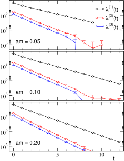
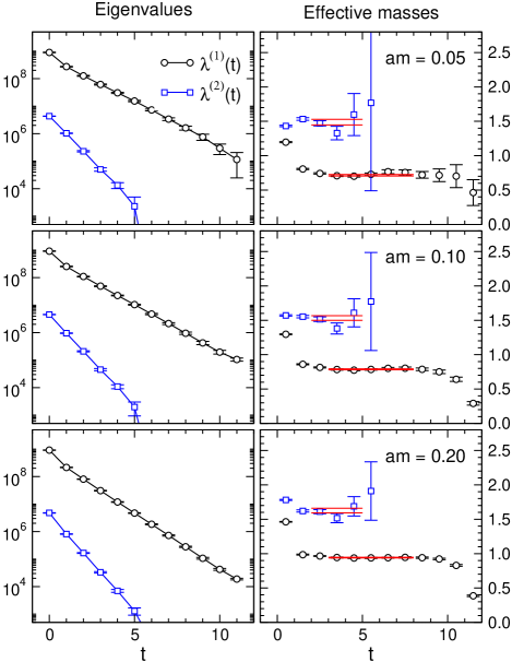
In Fig. 2 we show the positive parity parts of the three largest eigenvalues , and from the correlation matrix with the set of operators (15) constructed from the local interpolator. The exponential decay of all three eigenvalues is clearly seen and the slopes differ, most obviously for the ground state and the first excited state. We identify these signals with the nucleon, the Roper state and the next positive parity resonance . We remark that in the heavy quark region the latter two states belong to the same shell and hence must be approximately degenerate. However, given the fact that the masses of the excited states extracted from the second and the third eigenvalues are rather close, we perform an additional test that these eigenvalues represent different states.
It has been understood long ago that all Roper states form an excited -plet of SU(6). In this multiplet the parity of any two-quark subsystem is positive. The belongs to another multiplet, which contains both positive and negative parity two-quark subsystems. The two-quark subsystem in the brackets in , Eq. (11), has positive parity, while the subsystem in the brackets of has negative parity. Hence, applying the same type of smearings to the interpolator, we should see only the signal from the state, and no signals from the nucleon and the Roper. We have diagonalized a correlation matrix with the source combinations listed in (15) applied to the local interpolator and indeed observed a signal only in one eigenvalue. This signal is clearly compatible with the signal obtained with .
Before we discuss the effective masses and the fit procedures we used, let us address another important advantage of our source technique. In dongetal evidence for nucleon- ghost contributions (a quenching artifact) to the nucleon correlators at small quark masses was given. These contributions come with a negative coefficient and in dongetal had to be included explicitly in the multi-exponential fitting function of the correlator. In our correlation matrix analysis we find that the first and second eigenvalues are not at all affected by the ghost contributions, i.e. these correlators are positive and we observe undisturbed effective mass plateaus. Only the third and higher eigenvalues can become negative for large . Thus, the ghost contributions are disentangled from the ground state and the first excited state, i.e. the states we are interested in here.
Let us now present the effective masses as obtained from the correlation of the operators listed in Eq. (15). In Fig. 3 we show effective masses
| (16) |
for the first three eigenvalues (out of a total of four) with the data for in the left hand side column, in the center column and on the right hand side. We display the data for different quark masses from up to (top to bottom). The symbols show our numbers for the effective masses with statistical errors determined with the jackknife method. The horizontal lines in the plots represent our fit results: We plot the one standard deviation (s.d.) error band for the fitted mass. The band extends over the -interval which was used for the fit. We stress that these are not fits to the effective mass, but fully correlated fits to the propagators shown in Fig. 2. We discuss the details below.
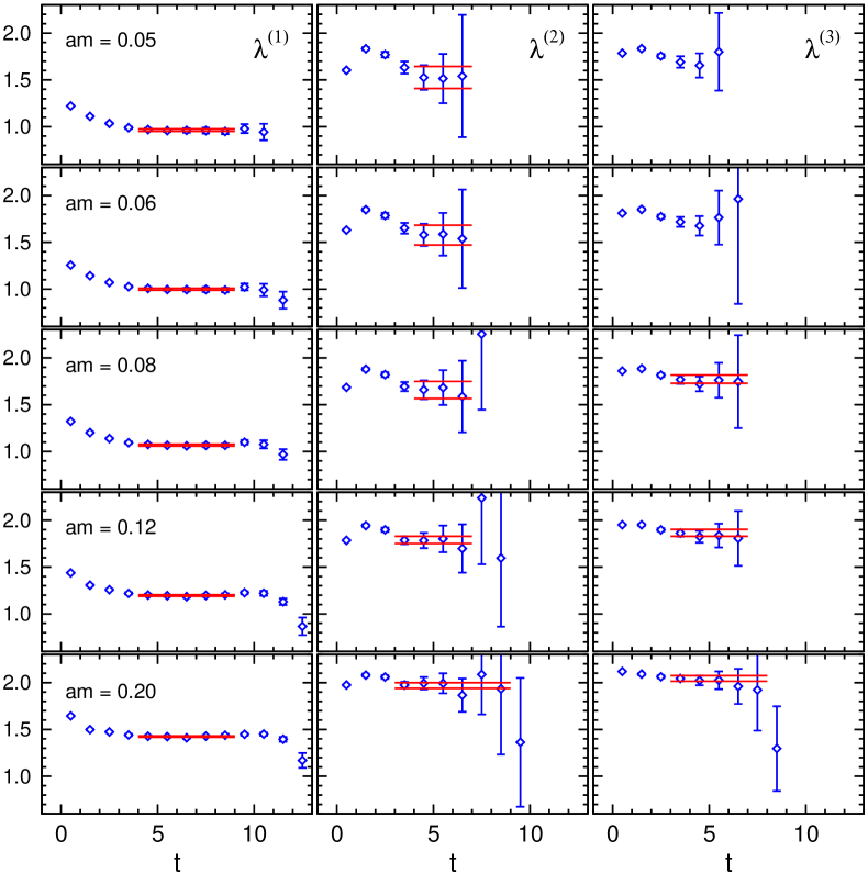
The signal for the ground state appears in the effective mass for which we show in the left hand side column. We find well pronounced plateaus. The fit range was chosen from to . For we observe contributions from higher excited states, while for one enters the crossing region where contributions from the negative parity states, which propagate backwards in time, start to mix with the positive parity signal.
The first excited state shows up in (center column). It is obvious, that here the statistical errors are larger than for the ground state, in particular for . This, however, is as expected for a heavier state which has a faster decreasing correlator, giving rise to a smaller signal to noise ratio already at not too large . However, also for the first excited state we find good plateaus in the effective mass. These plateaus extend from to for our largest mass and shrink to to for . We emphasize that there is a common interval in where all 3 plateaus are seen simultaneously. It is very satisfactory to see a credible effective mass plateau for the excited states and not to have to rely on the fits alone to extract their masses.
When inspecting the effective masses from the third eigenvalue one finds again good effective mass plateaus. The statistical errors are not larger than for the second eigenvalue and fits in similar -ranges can be performed. We did not fit the data for quark masses below where we no longer can exclude contributions from ghost states and observe a decreasing quality in the effective mass plateaus. When comparing the positions for the plateaus in the first and second excited states we find that they are rather close to each other. Only for the three largest masses, where the statistical errors are smaller, can we establish a mass splitting larger than one s.d. Also in nature the mass splitting between the first and second excited positive parity states ( and ) is relatively small.
Before we come to presenting the final mass values of our analysis we need to discuss the procedures we used for fitting the correlators. The exponential decay of the eigenvalues was fitted with the two parameter ansatz . Since the different values of are not statistically independent we used fully correlated fits. The statistical errors and the covariance matrix were determined with the jackknife method. The fit ranges were chosen such that they extend over those values of where we see a credible effective mass plateau. Changing the upper limit of the fit interval by does not affect the fit results (the variation is considerably less than one s.d.). Also an increase of the lower limit of the fit range changes the fit results by considerably less than one s.d. When decreasing the lower end of the fit interval, the result for the mass typically goes up by one s.d. This effect is obvious from the effective mass plots where one sees that for smaller one runs into the contributions of higher excited states. Our fits all have values smaller than 1 and the also stays below 1 when considering the changes in the fit range. Thus, the is not a very stringent criterion for determining the fit range and our choice based on the effective mass plateaus is rather conservative.
In our fits we carefully analyzed the possibility of normalizing our matrix as suggested by the generalized eigenvalue problem Eq. (9). In particular we tried the choices and found that the fits for the masses are unchanged within error bars. For the ground state the change was less than 0.3 s.d. and for the excited state less than 1 s.d. For we find a noticeable decrease in the quality of the effective mass plateaus, which comes from the fact the at the matrix which is used for the normalization already becomes affected by statistical noise. We cannot confirm any suppression of the effects from higher excited states and our results from the generalized eigenvalue problem are indistinguishable from the data obtained from the regular eigenvalue problem. In the further discussion we use the latter.
We experimented also with another possibility to fit our correlators. Based on the Hilbert space decomposition (7) we used an ansatz of the form
| (17) |
to fit an correlation matrix. The coefficients are chosen real, since the correlation matrix is real and symmetric. We find that the ansatz (17) can be applied successfully only for matrices. For larger correlation matrices the data of our ensembles used for testing the method are not accurate enough for the multi-parameter fit (17). The becomes large and we sometimes encountered convergence problems in the numerical minimization of the functional. For the case, however, the results from fitting the whole correlation matrix with (17) agree reasonably well with the fits of the eigenvalues. For the ground state mass the two results differ by less than one s.d. For the first excited state the difference is below one s.d. for rising to 1.5 s.d. at .
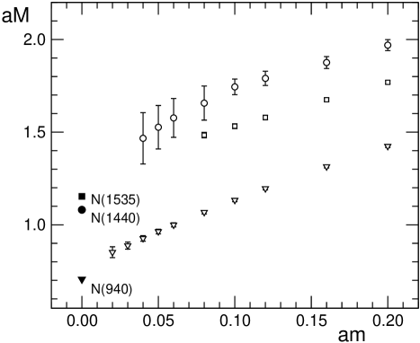
In Fig. 4 we show the fitted nucleon masses in lattice units as a function of the quark mass. Open triangles represent our data and the statistical error for the ground state and the filled triangle gives the experimental mass for the nucleon (converted to lattice units using the Sommer parameter). The open circles are the data for the first excited state and the corresponding filled circle represents the mass of the Roper . The open squares are the masses for the lowest negative parity state calculated on the same ensemble of configurations in broemmeletal . Note that the lower two data sets are for ground states of positive and negative parity and thus have smaller statistical errors. Although we do not attempt a chiral extrapolation of our data (this is deferred to a future large scale study of the nucleon system), our numbers seem to approach the experimental data reasonably well. For the quark mass range in our study the first excited, positive parity masses still remain above the negative parity, ground state data, but a trend towards a level crossing is plausible. We remark that the smallest quark mass where we can fit the excited nucleon, , corresponds to a pion mass of 450 MeV (see bgr ). Thus our preliminary data contradict a level crossing at 600 MeV as claimed in sasaki . Clearly further studies in larger volumes are important; such studies are in progress.
IV Example B: Excited rho meson
As another test of our approach we discuss the rho-meson and its radial excitation . Traditionally the has been studied with the vector current interpolator,
| (18) |
The same meson in the chiral symmetry broken regime should also be seen with the time component of the tensor interpolator,
| (19) |
The difference between the two is that they transform under different representations with respect to and Gloz1 . Again we use wide and narrow quark sources for both interpolators. Thus, for both interpolators (18), (19) we can build the 4 operators as listed in Eq. (10). However, the two combinations and give identical correlators and one of them can be omitted. Thus, we evaluate two correlation matrices, one for the vector interpolator and one for the tensor interpolator (the different spatial components are averaged). For both these interpolators we check whether the ground and radially excited states couple. When we diagonalize the matrix with either the interpolator (18) or the interpolator (19) we see a pronounced exponential decay only for the two larger (in magnitude) eigenvalues, and . The smallest eigenvalue does not show a clear effective mass plateau and becomes negative at small quark masses for large . This is a clear indication that this eigenvalue couples to an unphysical quenched ghost state Bardeen ; DeGrand .
In Fig. 5 we show the two larger eigenvalues and the corresponding effective mass plots obtained with the tensor current (19) for three different quark masses (, from top to bottom). We observe a clean exponential decay for both eigenvalues and corresponding plateaus in the effective mass plots. We remark, that results for the mass obtained with the vector current (18) agree within the error bars. Contrary to the baryon case, we observe only one radial excitation. Indeed, there is only a single one-node excitation for a meson with the given quantum numbers.
Like for the baryons, we apply a standard correlated single exponential fit to extract the meson masses. For the ground state the time interval is chosen to be (3,8), while for the excited state we use (2,5). The final results for the masses as a function of the quark mass are shown in Fig. 6. We find that the ground state approaches its experimental value reasonably well (the experimental data were converted to lattice units with the Sommer parameter scale).
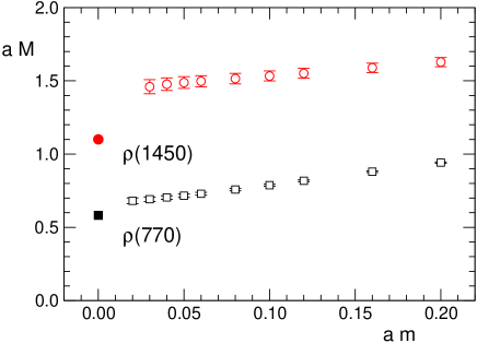
The excited state masses are considerably above their experimental value. There is, however, a plausible reason for this behavior. The sizes of hadrons which are not, or only weakly, affected by spontaneous chiral symmetry breaking can be estimated from the known string tension, which is approximately 1 GeV/fm. Hence the size of the -meson is expected to be below 1 fm, while the size of should be approximately 1.5 fm. The size of our lattice is 1.8 fm, which is clearly not enough for a precise measurement of the mass. The finite size effect cannot be neglected for the excited state and shifts the measured mass up as compared to the experimental value. A study of the rho system on larger lattices is in progress.
V Analyzing the operator content of the physical states
We have based our new approach on the working hypothesis that, when using the variational method, the excited states have a better overlap with a basis of operators that allow for a node in the spatial wave function. A crucial test of this assumption is to check whether indeed the ground state is built from a nodeless combination of our sources and the excited states do show nodes.
This question can be addressed by analyzing the eigenvectors of the correlation matrix (6). Let us denote by the -th eigenvector of the correlation matrix, and its eigenvalue is . Then we can define optimal operators by
| (20) |
with the mixing coefficients determined from the entries of the eigenvector via
| (21) |
where the asterisk denotes complex conjugation. The correlation matrix of the optimal operators is diagonal, i.e.
| (22) |
Thus, the operator has optimal overlap with the ground state, the operator has optimal overlap with the first excited state etc. By analyzing the coefficients we can thus learn about the structure of the state seen in the eigenvalue . In particular we can address the question whether there are nodes in the wave functions. As we have discussed in Section 2, a node occurs if there is a relative minus sign between the wide and the narrow quark source. For the nucleon system, where we work with the set of operators listed in (15), our working hypothesis implies that all coefficients have the same sign for the ground state, while for the excited states we expect relative signs.
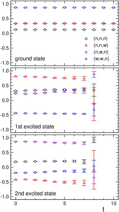
We determine the eigenvectors of at each value of . Since is real and symmetric, the eigenvectors can be chosen real. In Fig. 7 we display these eigenvectors for the nucleon analysis by plotting the (real) coefficients . In the top plot we show the numbers for the ground state (), in the middle plot the numbers for the first excited state () and in the bottom plot we display the second excited state (). The different symbols represent the mixing coefficients for the different basis operators and we use circles for , triangles for , upside down triangles for and squares for , all referring to the interpolator . The data we show are for quark mass . We remark that our eigenvectors are normalized to one, implying that
| (23) |
for the mixing coefficients. Furthermore, since is real symmetric, the eigenvectors are also orthogonal to each other for all .
It is obvious from the plot that also the mixing coefficients show plateaus. For the ground state these plateaus start at , while for the excited states they typically start at , where we also observed the onset of plateau-like behavior in the effective masses. Starting at the plateaus for the coefficients vanish for the excited states. At this the eigenvalues are already very small (they decay exponentially) and different eigenvectors start to mix. However, for all quark masses we observe long enough plateaus to clearly identify the mixing coefficients of the optimal operators.
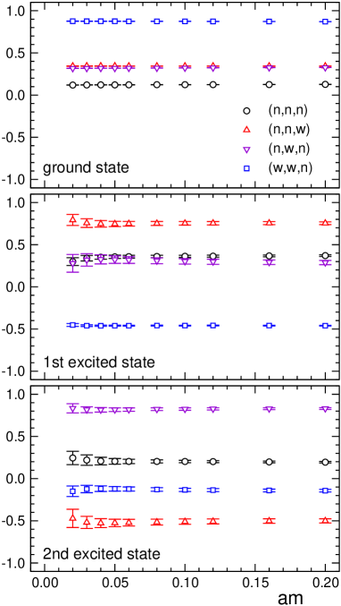
In Fig. 8 we show the mixing coefficients as a function of the quark mass. In particular we choose the values of the coefficients for time slice . We use the same symbols for the different basis operators as in Fig. 7 and again show from top to bottom the ground state, the first and the second excited state.
The top plot shows that for the ground state (the nucleon) all 4 mixing coefficients have the same sign and the wave function of the ground state does not have a node. For the two excited states the situation is clearly different. We find positive and negative coefficients, indicating that the wave function has a node. We stress that a linear combination of the profiles shown in Fig. 1, using the coefficients of Fig. 8 should not be literally interpreted as the true nucleon wave function. Firstly, our narrow and wide sources are not orthonormalized, and secondly they provide a much too small basis for mapping the details of a complicated three body wave function.
We performed the same analysis also for the eigenvectors of the correlation matrices we used for the rho meson. Again we confirm that the ground state has equal sign coefficients and thus is nodeless, while the excited state has relative signs between its coefficients indicating a node. Thus for both systems where we tested our method we could confirm that in the variational method combinations without node give rise to the ground state signal while the signal for excited states comes from combinations with a node.
VI Summary
We have presented a new approach to improving the spatial structure of operators used for hadron spectroscopy on the lattice. The central idea is to combine Jacobi smeared quark sources of different width in the variational approach. This combination allows for nodes in the spatial wave function and improves the signal from radially excited states. We have demonstrated the power of this approach by applying the method to a study of the lowest radial excitation of the nucleon, the Roper resonance, and to the radial excitation of the rho meson, . In both cases we clearly identify credible plateaus in the effective mass plots and are able to trace the signal of these states from the heavy quark region towards the chiral limit. It is reassuring to see clear effective mass plateaus also for the excited states, and the corresponding mass needs not be extracted from a multi-exponential fit. A simple single exponential fit is sufficient for extracting the mass from the decay of the second eigenvalue. When plotting the fitted masses as a function of the quark mass, the agreement with the experimental situation is reasonable. A large scale study with larger lattices and a systematic chiral extrapolation is in progress. We also note that it is possible to extend our method to the next radial excitations, with two nodes. For that one needs to use at least three different types of quark sources. We plan to study this extension of the method in the near future.
There are two physical implications of our preliminary observations:
(i) The fact that our numerical data for the first excited state can be plausibly interpreted as the Roper signal has an important consequence for the nature of this state: It implies that the Roper’s leading Fock component is a 3 quark state. A trend towards a level switching of the lowest positive and negative parity excited states is visible, which is consistent with the physical picture of Ref. GR .
(ii) In our data the quark mass dependence of the excited rho meson state is only weak. This implies that is only weakly affected by spontaneous breaking of chiral symmetry, in contrast to the lowest baryon states. This indicates that the physics of the excited meson states and of the lowest baryons is very different and that perhaps we observe a transition to the restoration of chiral symmetry in highly excited hadrons Gloz1 ; Gloz2 .
These are important conclusions and we expect that the application of our source techniques in a large scale study can lead to a deeper understanding of these issues from a lattice perspective.
Acknowledgements.
We want to thank Dirk Brömmel and Meinulf Göckeler for valuable discussions, and Stefan Schaefer for important contributions in the earlier stages of the BGR collaboration. The calculations were done on the Hitachi SR8000 at the Leibniz Rechenzentrum in Munich and we thank the LRZ staff for training and support. We acknowledge support by Fonds zur Förderung der Wissenschaftlichen Forschung in Österreich, projects P16310-N08 and P16823-N08 and by DFG and BMBF.References
- (1) F. X. Lee and D. B. Leinweber, Nucl. Phys. Proc. Suppl. 73, 258 (1999); F. X. Lee [LHPC], Nucl. Phys. Proc. Suppl. 94, 251 (2001); D. G. Richards et al. [LHPC], Nucl. Phys. Proc. Suppl. 109, 89 (2002); D. G. Richards, Nucl. Phys. Proc. Suppl. 94, 264 (2001); M. Göckeler et al. [QCDSF Collaboration], Phys. Lett. B 532, 63 (2002); S. Sasaki, T. Blum and S. Ohta, Phys. Rev. D 65, 074503 (2002); W. Melnitchouk et al., Phys. Rev. D 67, 114506 (2003); Nucl. Phys. Proc. Suppl. 119, 293 (2003); C. M. Maynard and D. G. Richards [UKQCD Collaboration], Nucl. Phys. Proc. Suppl. 119, 287 (2003); S. Sasaki et al., Nucl. Phys. Proc. Suppl. 119, 302 (2003); K. Sasaki, S. Sasaki, T. Hatsuda and M. Asakawa, Nucl. Phys. Proc. Suppl. 129-130, 212 (2004); R. G. Edwards, U. Heller and D. Richards, Nucl. Phys. Proc. Suppl. 119, 305 (2003); F. X. Lee et al., Nucl. Phys. Proc. Suppl. 119, 296 (2003).
- (2) S. J. Dong et al., hep-ph/0306199; Y. Chen et al., hep-lat/0405001.
- (3) S. Sasaki, Prog. Theor. Phys. Suppl. 151, 143 (2003).
- (4) D. Brömmel et al, hep-ph/0307073, (Phys. Rev. D, in print); Nucl. Phys. Proc. Suppl. 129-130, 251 (2004). hep-lat/0309036 (Nucl. Phys. Proc. Suppl., in print).
- (5) G.P. Lepage, Nucl. Phys. Proc. Suppl. 106, 12 (2002).
- (6) M. Asakawa, T. Hatsuda and Y. Nakahara, Prog. Part. Nucl. Phys. 46, 459 (2001).
- (7) C. Michael, Nucl. Phys. B 259, 58 (1985); M. Lüscher and U. Wolff, Nucl. Phys. B 339, 222 (1990).
- (8) S. Basak et al. [LHPC], Nucl. Phys. Proc. Suppl. 128, 186 (2004); Nucl. Phys. Proc. Suppl. 129-130, 209 (2004); R. Edwards et al. [LHP Collaboration], Nucl. Phys. Proc. Suppl. 129-130, 236 (2004).
- (9) C. Best et al., Phys. Rev. D 56, 2743 (1997); C. Alexandrou, S. Güsken, F. Jegerlehner, K. Schilling and R. Sommer, Nucl. Phys. B 414 (1994) 815; C. R. Allton et al. [UKQCD Collaboration], Phys. Rev. D 47 (1993) 5128.
- (10) P. Lacock, C. Michael, P. Boyle and P. Rowland [UKQCD Collaboration], Phys. Rev. D 54, 6997 (1996); C. Bernard et al. [MILC Collaboration], Nucl. Phys. Proc. Suppl. 129-130, 230 (2004); C. Aubin et al., hep-lat/0402030; J. N. Hedditch, D. B. Leinweber, A. G. Williams and J. M. Zanotti, Nucl. Phys. Proc. Suppl. 128, 221 (2004); C. McNeile and C. Michael [UKQCD Collaboration], hep-lat/0402012.
- (11) C. Gattringer, Phys. Rev. D 63 (2001) 114501; C. Gattringer, I. Hip, C.B. Lang, Nucl. Phys. B 597, 451 (2001).
- (12) P.H. Ginsparg and K.G. Wilson, Phys. Rev. D 25, 2649 (1982).
- (13) C. Gattringer et al. [Bern-Graz-Regensburg Collaboration], Nucl. Phys. B 677, 3 (2004); C. Gattringer, Nucl. Phys. B Proc. Suppl. 119, 122 (2003); C. Gattringer et al. [Bern-Graz-Regensburg Collaboration], Nucl. Phys. B Proc. Suppl. 119, 796 (2003).
- (14) M. Lüscher and P. Weisz, Commun. Math. Phys. 97, 59 (1985); Err.: 98, 433 (1985); G. Curci, P. Menotti and G. Paffuti, Phys. Lett. B 130, 205 (1983), Err.: B 135, 516 (1984).
- (15) C. Gattringer, R. Hoffmann and S. Schaefer, Phys. Rev. D 65, 094503 (2002).
- (16) G. E. Brown, J. W. Durso and M. B. Johnson, Nucl. Phys. A397, 447 (1983).
- (17) C. E. Carlson and N. C. Mukhopadadhyay, Phys. Rev. Lett. 67, 3745 (1991); Z. P. Li et al, Phys. Rev. D46, 70 (1992); L. S. Kisslinger and Z. Li, Phys. Rev. D51, R5986 (1995).
- (18) O. Krehl et al, Phys. Rev. C62, 025207 (2000).
- (19) T. D. Cohen and R. F. Lebed, Phys. Rev. D67, 096008 (2003) and references therein.
- (20) R. L. Jaffe and F. Wilczek, Phys. Rev. Lett. 91 232003 (2003); see however L. Ya. Glozman, hep-ph/0309092 (Phys. Rev. Lett., in print); T. D. Cohen, hep-ph/0402056.
- (21) L. Ya. Glozman and D. O. Riska, Phys. Rep. 268, 263 (1996); L. Ya. Glozman, W. Plessas, K. Varga and R. Wagenbrunn, Phys. Rev. D58, 094030 (1998); L. Ya. Glozman, Plenary talk at PANIC 99, Nucl. Phys. A663, 103 (2000).
- (22) L. Ya. Glozman, Phys. Lett. B587, 69 (2004).
- (23) W. Bardeen et al, Phys. Rev. D65, 014509 (2002).
- (24) T. DeGrand, Phys. Rev. D64, 094508 (2001).
- (25) L. Ya. Glozman, Phys. Lett. B475, 329 (2000); T. D. Cohen and L. Ya. Glozman, Phys. Rev. D65, 016006 (2002); T. D. Cohen and L. Ya. Glozman, Int. J. Mod. Phys. A17, 1327 (2002); L. Ya. Glozman, Phys. Lett. B539, 257 (2002); L. Ya. Glozman, Phys. Lett. B541, 115 (2002).