Phase Structure and Gauge Boson Propagator
in the radially active 3D compact Abelian Higgs Model

Abstract

Unfreezing the radial degree of freedom, we study the three-dimensional Abelian Higgs model with compact gauge field and fundamentally charged matter. For small quartic Higgs self coupling and finite gauge coupling the model possesses a first order transition from the confined/symmetric phase to the deconfined/Higgs phase separated at some hopping parameter $\kappa_{c}$. Latent heat and surface tension are obtained in the first order regime. At larger quartic coupling the first order transition ceases to exist, and the behavior becomes similar to that known from the London limit. These observations are complemented by a study of the photon propagator in Landau gauge in the two different regimes. The problems afflicting the gauge fixing procedure are carefully investigated. We propose an improved gauge fixing algorithm which uses a finite subgroup in a preselection/preconditioning stage. The computational gain in the expensive confinement region is a speed-up factor around 10. The propagator in momentum space has a non-zero anomalous dimension in the confined phase whereas it vanishes in the Higgs phase. As far as the gauge boson propagator is concerned, we find that the radially active Higgs field provides qualitatively no new effect compared to the radially frozen Higgs field studied before.

I Introduction

The lattice Abelian Higgs model with compact gauge fields (cAHM) has a wide variety of properties which makes it interesting from both the high energy physics Fradkin ; EinhornSavit and condensed matter physics AnomalousMatter point of view. The compactness of the gauge field gives rise to the presence of monopoles which are instanton-like excitations (topological defects) in three space-time dimensions. Being in the plasma state, monopoles and antimonopoles guarantee linear confinement of electrically charged test particles Polyakov . The topological defects are forming an oppositely charged double sheet along the minimal surface spanned by a Wilson loop. Due to screening, the free energy of this double sheet is proportional to the area of the minimal surface. As a result, electrically charged particles experience linear confinement.

In the case of the cAHM, the plasma state of the monopoles is realized, similar to pure cQED, at small values of the hopping parameter (coupling between matter and gauge fields) corresponding to the confined phase of cAHM. With respect to the Higgs degrees of freedom that phase is called symmetric. As the hopping parameter increases, the system enters the Higgs region, where e.g. the linear potential between test charges is suppressed. Correspondingly, in this phase monopoles and antimonopoles are bound into magnetically neutral dipoles, which provide at best only short-ranged interactions between the charged test particles. In other words, the presence of dynamical matter fields with charges in the fundamental representation of the gauge group leads to the effect of string breaking which results in a flattening of the potential at large charge separations. With respect to the gauge degrees of freedom the Higgs region is the deconfined region. The formation of magnetic dipoles in relation to the phenomenon of string breaking were studied both analytically in Ref. AnomalousMatter and numerically in Ref. Chernodub:2002ym . Note that the origin of monopole binding in the zero temperature case of cAHM₃ is physically different from the case of monopole binding at the finite temperature phase transition occurring in compact QED₂₊₁ without a dynamical Higgs field in the fundamental representation Agasian:2001an ; Binding ; CIS12 .

The effect of finite-temperature deconfinement on the photon propagator in ($2+1$)-dimensional cQED CIS3 ; Chernodub:2002gp ; Chernodub:2003bb and in zero-temperature cAHM in the London limit are rather similar Chernodub:2002ym . The propagator is described by a Debye mass and by an anomalous dimension which both vanish at the deconfinement transition regardless on its nature, which can be caused by finite temperature or by the presence of the matter fields. In both cases the transition is attributed to pairing of magnetic monopoles. The mass parameter of the propagator behaves differently in these cases since in the deconfined phase of the cAHM the gauge boson acquires a mass due to the Higgs mechanism whereas in the case of cQED this mechanism is of course absent.

The qualitative similarity of the form of the gauge boson propagators in cQED and in the cAHM, so far known in the London limit, immediately raises the question about the role of the Higgs field in the emergence of the anomalous dimension. Indeed, in the London limit of the cAHM the mass of the Higgs is infinite and the only active ingredient of the Higgs field is its compact phase. Away from the London limit the Higgs mass stays finite and the radial component of the Higgs field gains influence. In this paper we concentrate on the role of the radially active Higgs field on the properties of the gauge boson propagator in conjunction with the phase structure of the model.

The phase diagram of the cAHM in three dimension has been extensively studied both perturbatively (analytically) and numerically in the literature ref:phase ; ref:phase:prop1 ; ref:phase:prop2 . Already in the early studies ref:phase the changing nature of the phase transition due to radially active Higgs field has been addressed. The authors of Refs. ref:phase:prop1 ; ref:phase:prop2 have been concentrated on the continuum limit (studying large $\beta$) measuring among others the gauge boson mass from plaquette-plaquette correlators. As in our previous work we are studying here the propagator in momentum space which allows to establish easily whether a non-vanishing anomalous dimension exists.

The structure of the paper is as follows. Section II is devoted to the description of the model and to a sketch of its phase structure at two selected values of the coupling describing the quartic self-interaction of the Higgs field. The gauge fixing procedure and its inherent problems are reviewed in Section III where also a preconditioning method using a finite subgroup of the gauge group is proposed. Near the transition, the changing form of the photon propagator is analysed in Section IV. Our conclusions are given in Section V.

II The Model and its Phase Structure

II.1 Some properties of the model and its limiting cases

We consider the three-dimensional Abelian Higgs model with compact gauge fields $\theta_{x,\mu}\in[-\pi,\pi)$ living on links $l={x,\mu}$ and with fundamentally charged ($Q=1$) Higgs fields $\Phi_{x}\in\mathbb{C}$ on sites $x$ (a vector with integer Cartesian coordinates).

The Higgs field is written in the form

$$\Phi_{x}=\rho_{x}{\rm e}^{i\varphi_{x}}$$ (1)

where $\rho_{x}$ is its radial part and $\varphi_{x}$ its phase. The model is defined by the action

$$S=-\beta\sum_{P}\cos\theta_{P}-\kappa\sum_{x,\mu}\rho_{x}\rho_{x+\hat{\mu}}\cos(-\varphi_{x}+\theta_{x,\mu}+\varphi_{x+\hat{\mu}})+\sum_{x}(\rho_{x}^{2}+\lambda(\rho_{x}^{2}-1)^{2})\,,$$ (2)

where $\theta_{P}$ is the plaquette angle representing the curl of the link field $\theta_{x,\mu}$ and $\hat{\mu}$ is the unit vector in $\mu$ direction. $\beta$ is proportional to the inverse gauge coupling squared, $\beta=1/(a~{}g^{2})$, $\kappa$ is the hopping parameter and $\lambda$ the quartic Higgs self coupling. The so called London limit of that model has frozen radial Higgs length corresponding to $\lambda\to\infty$.

In that limit, at zero value of the hopping parameter $\kappa$, the model (2) reduces to the pure compact Abelian gauge theory which is known to be confining at any coupling $\beta$ due to the presence of the monopole plasma Polyakov . We call the low–$\kappa$ region of the phase diagram the ”confined region”. At large values of $\kappa$ (also called the ”Higgs region”) the monopoles should disappear because the requirement $\kappa\rightarrow\infty$ leads to the constraint $-\varphi_{x}+\theta_{x,\mu}+\varphi_{x+\hat{\mu}}=2\pi{}l_{x,\mu}$, with, in general, $l_{x,\mu}\in{Z\!\!\!Z}$. However, in the unitary gauge, $\varphi_{x}=0$, the above constraint along with the compactness condition for the gauge field, $\theta_{x,\mu}\in[-\pi,\pi)$, gives $\theta_{x,\mu}=2\pi{}l_{x,\mu}=0$, which, in turn, indicates the triviality of the model at large values of $\kappa$ in the London limit.

At large $\beta$ the model with $\lambda\to\infty$ reduces to the three dimensional $XY$ model which is known to have a second order phase transition at $\kappa^{XY}_{c}\approx 0.453$ XYphase between a symmetric and a Higgs phase. Indeed, in the limit $\beta\to\infty$ we get the constraint for the plaquette variable, $\theta_{P}\equiv{[\mathrm{d}\theta]}_{P}=2\pi n_{P}$, with $n_{P}\in{Z\!\!\!Z}$. The constraint implies $\mathrm{d}n=0$ (due to the nilpotency $\mathrm{d}^{2}=0$), which, in turn, gives $n=\mathrm{d}m$, where $m\in{Z\!\!\!Z}$ is a link variable. Thus, the constraint reduces to the equation $\mathrm{d}(\theta-2\pi m)=0$ which has a general solution of the form (in usual notations) $\theta_{x,\mu}=-\chi_{x+\hat{\mu}}+\chi_{x}+2\pi l_{x,\mu}$, where $\chi_{x}\in[-\pi,\pi)$ is a compact scalar field. The integer–valued vector field, $l_{x,\mu}\in{Z\!\!\!Z}$, is chosen in such a way that $\theta_{x,\mu}\in[-\pi,\pi)$. Fixing the unitary gauge we obtain that in the London limit and at large $\beta$ the action (2) reduces to the action of the $XY$–model, $S^{XY}=-\kappa\sum_{x,\mu}\cos(-\chi_{x}+\chi_{x+\hat{\mu}})$, where the scalar angle $\chi$ plays the role of the spin field in that model.

From our previous studies in the London limit at $\beta=2.0$ Chernodub:2002ym ; Chernodub:2002en we know that the transition from the confined to the Higgs region is signalled by a rapid drop of the monopole density. In addition, a string breaking phenomenon affecting fundamental test charges (being in the same representation as the fundamentally charged matter fields) has been observed which are bound by a linear (string) potential in the confined region. While the drop of the monopole density signals onset of deconfinement, the anomalous dimension of the photon propagator turning to zero at the same critical $\kappa_{c}$ shows the transition from the symmetric to the Higgs region, whereas the observed non-zero photon mass at larger $\kappa$ is simply due to the onset of normal mass generation by the Higgs effect.

However, we could not confirm that this crossover is accompanied by an ordinary phase transition. It cannot be excluded that the transition is second order with a very small negative critical exponent or possibly of Kosterlitz-Thouless type.

Including a fluctuating radial degree of freedom $\rho_{x}$ (at small $\lambda$) changes the situation strongly. For fixed $\lambda$ a first order phase transition is known to exist ref:phase:prop2 from the symmetric to the Higgs phase in the $\beta$–$\kappa$ plane accompanied by the monopole density approaching zero, similar to our previous studies of the $3D$ SU(2)-Higgs model Ilgenfritz:1995sh ; Gurtler:1996wx . With increasing quartic Higgs self coupling the first order transition becomes weaker and ends at a certain critical $\lambda_{c}$ Gurtler:1997hr . Above that critical self coupling the phase structure of the compact Abelian Higgs model has been investigated in ref:phase:prop1 for relatively large $\beta$ with practically vanishing monopole density. In a very recent study wenzel the location of $\lambda_{c}$ has been established for a smaller (inverse) gauge coupling $\beta=1.1$ as

$$0.030<\lambda_{c}<0.032\,.$$ (3)

II.2 Two regimes of Higgs self coupling

In the present work we consider the gauge coupling $\beta=2.0$ corresponding to a smaller lattice spacing $a$ than in Ref. wenzel . For this gauge coupling the endpoint of the transition is found to be future

$$\lambda_{c}\approx 0.009(1)\,.$$ (4)

More details of this phase transition study will be presented elsewhere. We restricted the Higgs self coupling to two values $\lambda=0.005$ (representing the first order transition regime) and $\lambda=0.02$ (representing the continuous transition region).

In our simulations one complete Monte Carlo update consists of a Higgs and a gauge field update in alternating order. For the gauge fields a usual Metropolis algorithm has been applied. The algorithm was adjusted (during the thermalization) to ensure an acceptance rate of about 50 per cent. Representing the Higgs field as real two-component vector a heat-bath algorithm similar to the method described in Bunk:xs has been used. Additional overrelaxation steps have been applied to the Higgs field. Since the autocorrelation changes marginally with the number of reflection steps not more than two reflections per heatbath update have been used.

In order to locate the phase transition and to quantify its strength we consider for the present purposes only the gauge invariant average Higgs modulus squared

$$\rho^{2}=\frac{1}{L^{3}}\sum_{x}\rho_{x}^{2}\,$$ (5)

($L$ is the linear extent of the lattice) and evaluate its vacuum expectation value $\langle\rho^{2}\rangle$. For the Higgs modulus squared one can consider the susceptibility

$$C_{\rho^{2}}=L^{3}\,\left\{\langle(\rho^{2})^{2}\rangle-\langle\rho^{2}\rangle^{2}\right\}$$ (6)

and the Binder fourth cumulant as function of $\kappa$ (at fixed $\beta$ and $\lambda$) near criticality for different lattice volumes. Widely used multihistogram reweighting methods have also been applied in our work in order to determine the pseudocritical hopping parameter $\kappa_{c}$.

As one example we show here in Fig. 1 for the two $\lambda$ values

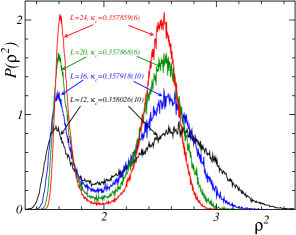
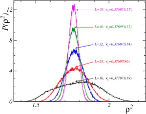
Figure 1: $\rho^{2}$ histograms at pseudocriticality: (a) for $\lambda=0.005$ with $\kappa_{c}$ fixed according to the equal height criterion and (b) for $\lambda=0.02$ according to the maximal susceptibility criterion.

the histograms $P(\rho^{2})$ (normalized to unit area) from all data at different $\kappa$ values near $\kappa_{c}$ and lattice sizes $L^{3}$ reweighted to the respective pseudocritical hopping parameter $\kappa_{c}$. In case (a) $\kappa_{c}$ for the lower $\lambda$ has been fixed according to the equal height condition applied to the two-state histogram. In case (b) for the larger $\lambda$ value $\kappa_{c}$ has been determined according to the condition that the susceptibility $C_{\rho}$ takes its maximum. One observes that in Fig. 1 (a) the two peaks become more pronounced with increasing volume whereas the distance between the maxima only marginally decreases. The tunnelling frequency between the two coexisting phases in a finite system (obtained from the autocorrelation function of $\rho^{2}$) rapidly decreases with increasing volume. At a lattice volume $40^{3}$ (the one used for the propagator measurements to be discussed later) no tunnelling has been observed. This has allowed us to cleanly study and contrast the respective propagators of the competing phases.

The first order transition is characterized by a finite jump $\Delta\langle\rho^{2}\rangle$ of the average Higgs modulus squared, a two-state signal at pseudocriticality, surviving in the infinite volume limit. This jump is related to the latent heat of the first order transition

$$\frac{L_{\rm heat}}{g_{3}^{2}}=\frac{1}{2}\kappa\beta\,\Delta\langle\rho^{2}\rangle$$ (7)

with $g_{3}^{2}=1/(a\beta)$, $a$ is the lattice spacing. In the symmetric phase $\langle\rho^{2}\rangle$ is nearly constant as a function of $\kappa$. In contrast to this, on the Higgs side of the transition $\langle\rho^{2}\rangle$ increases approximately linear with $\kappa$.

Fig. 1 (a) clearly demonstrates that the transition is first order at $\lambda=0.005$. We also have observed that the maximum of the susceptibility (not shown here) increases linearly with the volume. Following Ref. ref:phase:prop2 we can estimate the dimensionless surface tension from the shape of the equal height histogram:

$$\sigma=\frac{\beta^{2}}{2L^{2}}\ln\frac{P_{\rm max}(\rho^{2})}{P_{\rm min}(\rho^{2})}\,.$$ (8)

Here $2L^{2}$ is the dimensionless area of two minimal surfaces splitting the periodic lattice into two regions filled with the two pure phases being in coexistence; $P_{\rm max}(\rho^{2})$ and $P_{\rm min}(\rho^{2})$ are the maximal/minimal value of the histogram, respectively. An extrapolation to the infinite volume limit (taking into account the leading $1/V$ corrections) leads to the following estimates of the latent heat and of the dimensionless surface tension

$$\frac{L_{\rm heat}}{g_{3}^{2}}=0.320(2)\,,\quad\sigma=0.0121(3)\,.$$ (9)

Fig. 1 (b) shows immediately that at $\lambda=0.02$ a first order transition does not exist. As indicated in the figure the histogram merges into definitely one maximum at larger lattice volume. Therefore there is no non-vanishing latent heat. The width of the histogram reduces with increasing volume. Within errors, the susceptibility for the largest studied volumes (again not shown) does not change as function of the volume. Fitting the susceptibility at the maximum for lattices from $L=32$ to $L=48$ by the function $C_{\rho^{2}}=AL^{\gamma}$ gives $\gamma=-0.014(40)$ with $\chi^{2}/d.o.f.=0.9$. Including a subleading correction we obtain $\gamma=-0.012(27)$ for lattices from $L=16$ to $L=48$. This excludes a second order transition with a critical exponent differing significantly from zero. The transition is similar as the one found in the London limitChernodub:2002ym .

II.3 The monopole density near criticality and autocorrelation estimates

In addition to $\rho^{2}$ we also consider the monopole degrees of freedom constructed out of the gauge fields. Using the differential form notation we consider the monopole charges as the 0-form $\mbox{}^{\ast}j\in{Z\!\!\!Z}$ defined on the sites dual to the lattice cubes $c$ DGT where it is evaluated as follows:

$$j=\frac{1}{2\pi}\sum\limits_{P\in\partial c}{(-1)}^{P}\,{[\theta_{P}]}_{\mathrm{mod}\,2\pi}\,.$$ (10)

The factor ${(-1)}^{P}$ takes the plaquette orientations relative to the (outer) boundary of the cube into account, and the notation $[\cdots]$ means taking the integer part modulo $2\pi$. The 2-form

$$p[j]={[\mathrm{d}\theta]}_{\mathrm{mod}\,2\pi}$$ (11)

corresponds to the Dirac strings living on the links of the dual lattice, which are dual to the plaquettes where the r.h.s. is evaluated. The Dirac strings are either forming closed loops or they are connecting monopoles with anti-monopoles, $\delta\mbox{}^{\ast}p[j]=\mbox{}^{\ast}j$. Whereas $\mbox{}^{\ast}j$ is gauge invariant, the 2-form $p[j]$ is not.

The simplest quantity describing the behavior of the monopoles is the average monopole density

$$\rho_{\rm mon}=\frac{1}{L^{3}}\sum_{c}|j_{c}|\,,$$ (12)

where $j_{c}$ is the integer valued monopole charge inside the cube $c$ defined in Eq. (10).

The measured value of the monopole density at smaller and larger $\lambda$ are shown in Fig. 2 for two lattice volumes $20^{3}$ and $40^{3}$ as a function of $\kappa$.

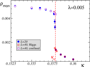
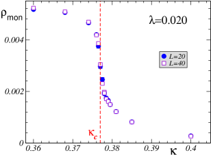
(a)	(b)

Figure 2: Monopole density $\rho_{\rm mon}$ near $\kappa_{c}$ for $20^{3}$ and $40^{3}$ lattice at $\lambda=0.005$ (a) and $\lambda=0.02$ (b).

The vertical lines are drawn to mark the pseudocritical $\kappa_{c}$. Clearly the monopole density jumps from a nearly constant, finite value to a small value crossing the transition from the confined to the Higgs phase. At larger lattices a metastability region is observed (in the form of a small hysteresis cycle) continuing the confined and Higgs phase, respectively, into the critical region. For the lattice $40^{3}$ the two metastable states at $\kappa_{c}$ are selected by the starting conditions of the Monte Carlo run. At higher $\lambda$ we observe a rapid but smooth decrease vs. $\kappa$ near $\kappa_{c}$ precisely as in the London limit.

Finite size effects on the monopole density are very small, therefore, also the susceptibility of the monopole density is practically unchanged with increasing lattice size. As we have found earlier, the remaining non-vanishing density above the transition is due to dipole pairs forming a dilute dipole gas. We will keep to these two values of the quartic self coupling in order to study the influence of the different transition regimes on the photon propagator.

Finally we show in Fig. 3

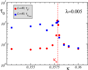
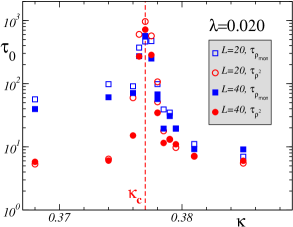
(a)	(b)

Figure 3: The integrated autocorrelation times $\tau_{O}$ of $\rho^{2}$ (circles) and $\rho_{\rm mon}$ (squares), (a) in the first order region, (b) in the continuous transition region.

the integrated autocorrelation time $\tau_{O}$ (for $\rho^{2}$ and $\rho_{\rm mon}$) as function of $\kappa$. We recall that the autocorrelation time of an observable $O$ is defined as

$$\tau_{O}=\frac{1}{2}+\sum_{\tau=1}^{N}C_{O}(\tau)\,,\quad N\gg 1$$ (13)

in terms of the autocorrelation function $C_{O}(\tau)$. In general, $C_{O}(\tau)$ is defined as

$$C_{O}(\tau)=\frac{\langle O_{t}O_{t+\tau}\rangle-\langle O_{t}\rangle^{2}}{\langle O_{t}^{2}\rangle-\langle O_{t}\rangle^{2}}$$ (14)

where the observable $O$ as measured at Monte Carlo “time” $t$ is folded with $O$ measured at $t+\tau$. On the confinement side the autocorrelation time for the monopole density is much larger than for the Higgs modulus squared. For both quantities $\tau_{O}$ reaches ${\mathcal{O}}(100)$ in the first order regime and up to ${\mathcal{O}}(1000)$ at critical coupling at larger $\lambda$. Since for the latter case the autocorrelation times of both $L=20$ and $L=40$ cubic lattices are roughly the same, we have not to worry about critical slowing-down. These autocorrelation times have been used to select statistically (almost) independent configurations for measurements of the photon propagator in the respective cases of the quartic Higgs self couplings.

III Landau gauge fixing with overrelaxation revisited

III.1 Landau gauge and Dirac strings

In order to calculate the (gauge dependent) photon propagator directly, a special gauge has to be chosen, in our case the minimal Landau gauge. This gauge is defined by finding the global maximum of the gauge functional

$$F=\frac{1}{N_{\rm links}}\sum_{x,\mu}\cos(\theta^{G}_{x,\mu})\rightarrow{\rm max}\,.$$ (15)

The gauge field and Higgs field angles have to been transformed into this gauge within gauge transformations $G$ with elements $g_{x}=\exp(i\omega_{x})$ acting as

$$\theta_{x,\mu}^{G} = \left(\omega_{x}+\theta_{x,\mu}-\omega_{x+\mu}\right)_{2\pi}\,.$$ (16)

$$\varphi_{x}^{G} = \left(\varphi_{x}+\omega_{x}\right)_{2\pi}$$ (17)

until the condition (15) is satisfied. The notation $\left(\dots\right)_{2\pi}$ indicates that values are restricted to the interval $[-\pi,\pi)$ (modulo $2\pi$).

Every gauge transformation can be decomposed into a sequence of local gauge transformations on each lattice site which would increase the sum (15) restricted to neighboring links. The corresponding angle $\omega_{x}$ is found easily as

$$\tan\omega_{x}=\frac{\sum_{\mu}\left(\sin\theta_{x,\mu}-\sin\theta_{x-\hat{\mu},\mu}\right)}{\sum_{\mu}\left(\cos\theta_{x,\mu}+\cos\theta_{x-\hat{\mu},\mu}\right)}\,.$$ (18)

The efficiency of the full optimization procedure depends crucially on the landscape of the gauge functional in the space of all gauge transformations. We have applied the local gauge transformation in a checkerboard fashion (based on a separation into odd and even sublattices). It turns out that overrelaxation allows us to speed up the finding of a local maximum with respect to full gauge transformations $G$. This was realized multiplying the gauge angles $\omega_{x}$ by an overrelaxation parameter $1<\eta<2$. Note that the extreme case $\eta=2$ does not change the local gauge functional at all because it corresponds to a microcanonical update with respect to the gauge functional $F$. Fastest convergence was obtained for $\eta$ values of about 1.8-1.9 in agreement with earlier findings Chernodub:2002gp .

This algorithm will in general not lead to the absolute (global) maximum of the gauge functional $F$ (15). Typically it will get stuck in one of the local maxima, which are called Gribov copies of each other and of the (unknown) true maximum. As long as this non-uniqueness influences the non-gauge-invariant observable of interest, this is the origin of the so-called Gribov problem. Practically, it is partially cured by repeating the same gauge fixing procedure, applying it to random gauge copies of the original Monte Carlo configuration. The local maximum with the largest value of $F$ is taken as the tentative global maximum. This rests on the assumption that one of these random gauge copies might be situated in the basin of attraction of the global maximum.

The number of gauge equivalent configurations produced to restart the gauge fixing is denoted as $N_{G}$, and the iterative gauge fixing generically leads to really different maxima. We have then to content with the best out of all $N_{G}+1$ local maxima of the gauge functional, and the observable of interest (the photon propagator) will depend on $N_{G}$.

For the purpose of the following discussion $\eta=1.8$ has been chosen. It will become clear that this choice is not advantageous. A closer investigation of the gauge fixing procedure reveals a direct relationship between the achieved value of the gauge functional and the density of leftover (gauge dependent) Dirac strings 

$$n_{\rm Dirac}=\frac{1}{N_{\rm links}}\sum_{{}^{*}P}|p_{P}[j]|$$ (19)

where the sum is taken over the links ${}^{*}P$ of the dual lattice. In particular, maximizing the gauge functional leads to a minimization of the Dirac string density as discussed in Chernodub:2002gp . Note that this dependence is a result of the local gauge fixing procedure which blindly acts with respect to the Dirac string content.

The different behavior in the confined and Higgs (deconfined) phase is demonstrated in Fig. 4

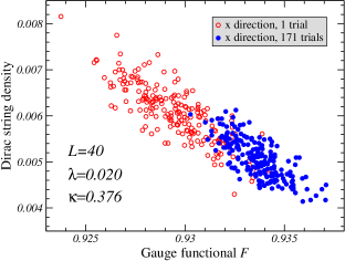
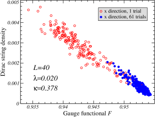
(a)	(b)

Figure 4: (a) The highest gauge functional after 1 trial ($N_{G}=0$) and 171 trials ($N_{G}=170$) on the confined side of the continuous transition near $\kappa_{c}$; (b) the same with 1 and 61 trials, respectively, on the Higgs (deconfined) side.

showing the Dirac string density (separately measured with respect to different directions, but shown only for the $x$ direction) vs. the values of the gauge functional for an ensemble of 195 independent configurations. Both quantities have been finally achieved after inspecting the first or the best copy among $N_{G}+1$ local maxima of the gauge functional $F$.

From the figures it is clear, that in both regions with a single attempt the best realization of the gauge fixing has never been found. In the Higgs region corresponding to deconfinement ($\kappa=0.378$), with sufficiently many copies $N_{G}$ created for selection, in most cases the relative maximum of the gauge functional is located in a small interval just below 0.955 with a Dirac string density below 0.001. Here one can hope finally to catch the global maximum accompanied by a minimal density of Dirac strings with a modest increase of the number of trials.

In the confining phase the behavior is different. Even with 170 copies under inspection, the reduction of the Dirac string density and the increase of the gauge functional is less efficient. Although the average of the gauge functional is shifted towards higher values its spread compared to the original spread remains rather large and the highest values of 0.938 are scarcely reached. The relative decrease of the density of Dirac strings is poor. We will see soon that such a far-from-perfect gauge fixing strongly influences the propagator.

On the other hand, from the absolute values of $n_{\rm Dirac}$ it can be concluded that Dirac lines wrapping around the torus are absent. They cannot be blamed to spoil the photon propagator, an effect which otherwise could be argued to be unphysical . Essentially the same observations can be made in the case of the smaller $\lambda$ value (in the neighborhood of the first order transition), but here without the possibility to simply separate out the ”physical case”. Thus, it is conceivable that a smarter local gauge fixing procedure could be able to reduce the Dirac string density to a (gauge independent) minimum.

Before any gauge fixing is attempted, the gauge dependent Dirac strings are either open lines (forming Dirac lines connecting monopoles and antimonopoles) or closed loops. In the confined phase these strings form huge clusters where the individual lines and loops cannot be resolved. It is impossible to uniquely identify throughgoing lines/loops at points where more than two Dirac strings meet. After some local maximum of the gauge functional has been found, the number of closed loops has decreased considerably. Closed loops have the chance even to be gauged away. Open strings which connect gauge-independent monopole-antimonopole pair positions are only able to minimize their length (number of contributing strings) during the gauge fixing procedure.

In an idealized picture with no leftover loops, a local maximum of $F$ is associated with a realization of Dirac lines necessary to connect monopole pairs. The global maximum then corresponds to a minimal realization. In the confined phase we have a dense plasma of monopoles and antimonopoles with total charge zero. Hence a lot of pairings are possible which corresponds to a huge number of local maxima of the gauge functional. On the Higgs side (deconfinement) only a small number of nearby (in lattice distances) monopole-antimonopole pairs (a dilute dipole gas) is left. Consequently, the number of local maxima is much lower than in the confined case. This picture explains why it is much more unlikely to find the global maximum of $F$ in the confined phase compared to the deconfined phase. The problem of the gauge fixing in the confined phase belongs to the class of complex systems similar in complexity to the zero temperature states in spin glasses.

III.2 Choice of the algorithm

The gauge fixing algorithm with continuous compact fields is very costly. To speed up the algorithm several refinements have been done. The implementations were tested for $\kappa<\kappa_{c}$ (confined side) because this is the most critical region. Firstly, we tested the effect of restricting the link variables to the discrete subgroup $\mathbb{Z}_{N}\subset U(1)$, i.e. mapping first the gauge field variables to the closest $\mathbb{Z}_{N}$ realization. Consequently, the gauge transformations were restricted to $\mathbb{Z}_{N}$, too. We observed that approximating gauge field angles by 1 byte arrays ($N=256$) gave, on the average, a lower gauge functional than using continuous compact fields. Using 2 byte arrays ($N=65536$) the gauge functionals resulting from gauge fixing using continuous angles and discrete angles, respectively, coincide within statistical errors for some tested $\eta$ values.

Secondly, we used a preselection strategy. The $N_{G}+1$ gauge fixing attempts can be performed at some chosen overrelaxation parameter $\eta\lesssim{}2$ with a rather weak stopping criterion, i.e. the lower limit for the change of the gauge functional was still relatively large. The actual choice of the best $\eta$ for the preselection stage is discussed below. Afterwards, among the non-precisely gauge-fixed copies the trial with the highest gauge functional was taken up again, and a final gauge fixing with a strong stopping criterion was applied stepping back now to a smaller overrelaxation parameter $\eta=1.90$ leading to fastest final convergence during the final-gauge fixing stage. The intuition behind this method is that during the preselection stage a certain pairing of (anti-)monopoles is already chosen and the fine tuning of the link angles is left to the second stage.

Both ideas have been then combined to use discrete gauge fixing in the preselection stage and to apply continuum gauge fixing only to the best copy obtained in the result of preselection. For this purpose, a $\mathbb{Z}_{N}$ realization of the gauge field was used first to construct a suitable $\mathbb{Z}_{N}$ gauge transformation, applying the weak convergence criterion. Then, embedding the optimal discrete gauge transformation into $U(1)$ as an initial guess and returning to the true $U(1)$ gauge field, the final continuous gauge fixing was done only for the most promising copy. The described combined procedure is called optimized gauge fixing in Fig. 5. Sensible stopping limits depend on the gauge functional landscape and thus on the lattice size and the coupling parameters. They had to be chosen appropriately. Using that optimized gauge fixing a speed-up of roughly a factor 10 has been found.

As mentioned above using $\eta=1.8$ might be not a good choice. This is demonstrated in Fig. 5

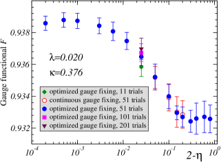
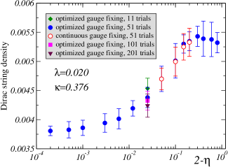
(a)	(b)

Figure 5: (a) The average of the maximal gauge functional per configuration as function of $\eta$; (b) the same for the minimal Dirac string density. Continuous gauge fixing is selfexplaining. For details of the optimized gauge fixing see the text.

showing the $\eta$ dependence of the gauge functional $F$ and of the Dirac string density $n_{\rm Dirac}$ for $\eta$ values near (but below) two using 20 independent measurements. This dependence has been overlooked in our previous studies. Only for the largest $\eta$ values (very close to $\eta=2$) we seem to reach a new level of performance (higher gauge functional, lower Dirac string density). In the figure for some selected $\eta$ values we also show measurements comparing the results achieved with the optimized algorithm (using discrete stage for preselection and preconditioning) with the standard algorithm using only continuous gauge transformations. As mentioned above, within statistics the results coincide. At $2-\eta=0.02$ we show in addition how the change of $N_{G}$ influences both gauge functional and Dirac string density. In order to reach the same level by increasing the number of copies $N_{G}$ turned out to be much more expensive in computing time than increasing $\eta$. Choosing $\eta$ close to 2 or, alternatively, applying several $\eta=2$ (the exactly microcanonical case) and $\eta<2$ overrelaxation steps in alternating order, has led to a very similar convergence behavior. In the first case the $\eta$ value was tuned and in the latter case we have adjusted the number of microcanonical steps interspersed between the overrelaxation steps in order to obtain the largest average of the final gauge functional. The iteration number $N_{\rm iter}$ (iteration of local gauge transformations) needed in order to reach a certain gauge functional has been found to be about the same in both cases.

Unfortunately, $N_{\rm iter}$ increases very fast if one tries to get at higher values of the gauge functional using one of these methods. Comparing $\eta=1.997$ with $\eta=1.80$ that number rises by a factor of 15 to 20. The highest value of $\eta$ which has led to an affordable $N_{\rm iter}$ in order to complete at least 50 independent measurements for the photon propagator was actually $\eta=1.997$ . Using this value one reaches the edge of a new level of performance both in the gauge functional and the Dirac string density indicating that the effect of increasing $\eta$ further should become small. Note that for $\eta$ close to 2 the algorithm behaves similar to a simulated annealing technique. Which of the techniques is computationally favorable, remains to be studied. It has been observed that increasing $\eta$ is much more efficient than increasing the number of trials $N_{G}+1$ using as measure the computational workload, i.e. the total number of updates of the local gauge transformations $(N_{G}+1)\times N_{\rm iter}$.

After these detailed studies we have chosen the following parameters as a standard to perform the Landau gauge fixing in the measurements of the gauge boson propagator: As weak stopping criterion the change of the gauge functional between two iterations had to become less than $1/(3\times 40^{3})$, as strong stopping criterion we used $10^{-8}/(3\times 40^{3})$. The number of Gribov copies at $\eta=1.997$ was chosen to be 51.

IV Results for the propagator near criticality

The photon propagator is the gauge-fixed ensemble average of the following bilinear in $\tilde{A}$,

$$D_{\mu\nu}({\vec{p}})=\langle\tilde{A}_{{\vec{k}},\mu}\tilde{A}_{-{\vec{k}},\nu}\rangle\,,$$ (20)

where $\tilde{A}$ is the Fourier transformed lattice gauge potential (in lattice momentum space) related to the gauge links $\theta_{x,\mu}$ (fixed to minimal Landau gauge in coordinate space) via 

$$\tilde{A}_{{\vec{k}},\mu}=\left(\frac{1}{L^{3}}\right)^{1/2}\sum\limits_{x}\exp\Bigl{(}2\pi i~{}\sum_{\nu=1}^{3}\frac{k_{\nu}(~{}x_{\nu}+\frac{1}{2}\delta_{\nu\mu}~{})}{L_{\nu}}\Bigr{)}~{}\sin\theta_{x,\mu}\,,\quad k_{\mu}=0,\pm 1,...,\pm\frac{L_{\mu}}{2}\,,$$ (21)

The vectors of lattice momenta ${\vec{p}}$ on the left hand side of (20) are related to the integer valued Fourier momenta vector ${\vec{k}}=(k_{1},k_{2},k_{3})$ as follows:

$$p_{\mu}(k_{\mu})=\frac{2}{a}\sin\frac{\pi k_{\mu}}{L_{\mu}}\,,\quad\vec{p}=(p_{1},p_{2},p_{3})\,.$$ (22)

Thus the lattice equivalent of the same continuum $p^{2}$ can be realized by different vectors $\vec{k}$ which eventually could reveal a breaking of rotational invariance.

Assuming reality and rotational invariance the most general tensor structure of the continuum propagator is

$$D_{\mu\nu}({\vec{p}})=P_{\mu\nu}({\vec{p}})~{}D(p^{2})+\frac{p_{\mu}p_{\nu}}{p^{2}}\frac{F(p^{2})}{p^{2}}$$ (23)

with the three-dimensional transverse projection operator

$$P_{\mu\nu}({\vec{p}})=\delta_{\mu\nu}-\frac{p_{\mu}p_{\nu}}{p^{2}}\,.$$ (24)

The two scalar functions (form factors) $D(p^{2})$ and $F(p^{2})$ can be extracted on the lattice from $D_{\mu\nu}({\vec{p}})$ by projection. Since $D_{\mu\nu}({\vec{p}})$ is only approximately rotationally invariant, the form factors may be scattered rather than forming a smooth function of $p^{2}$. When the Landau gauge is exactly fulfilled $F(p^{2})\equiv 0$. On the lattice, this is actually the case as soon as one of the local maxima of the gauge functional (15) is reached, with an accuracy which directly reflects the precision at stopping of the gauge fixing iterations. There is no possibility to monitor through $F(p^{2})$ to what extent the global maxima have been successfully found.

In order to measure the propagator, for lattice size $40^{3}$, we have considered 50 (almost) independent configurations (separated by 720 Monte Carlo sweeps) on the confined/symmetric side and 100 configurations (separated by 360 Monte Carlo sweeps) on the deconfined/Higgs side near $\kappa_{c}$ for the two representative cases of $\lambda$ ($\lambda=0.005$ and $0.02$). There were several reasons for choosing this lattice size. A large lattice reduces the influences of the boundary and leads to smaller variances in certain observables, e.g. the monopole density. Furthermore, in the first order regime tunnelling was prohibited (mixed phases during measurement) and the propagator properties of both phases in a metastability region could be independently studied. Finally, the relatively large size allows to measure the propagator for more realizations of very small momenta where the propagator in the confined phase is most sensitive.

In Fig 6

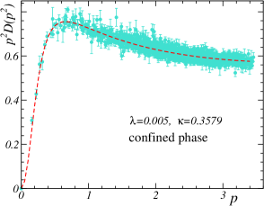
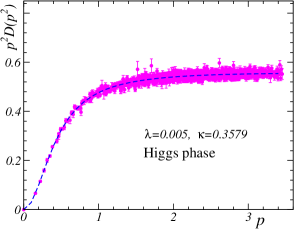
(a)	(b)

Figure 6: Momentum dependence of the photon propagator form factor $D(p^{2})$ multiplied by $p^{2}$ for $\lambda=0.005$ at $\kappa_{c}=0.3579$ together with the fit (25) in the confined/symmetric phase (a) and in the deconfined/Higgs phase (b).

we present as example the form factor $D(p^{2})$ multiplied by $p^{2}$ measured at the same $\kappa=\kappa_{c}$ in the metastability region. The system was found either in the confined/symmetric and the deconfined/Higgs phase depending on the initial conditions of the Monte Carlo run.

To describe the scalar function $D(p^{2})$ quantitatively we applied the following fit ansatz

$$D(p^{2})=\frac{Z\,m^{2\alpha}}{\beta\left[p^{2(1+\alpha)}+m^{2(1+\alpha)}\right]}+C\,,$$ (25)

where $Z$, $\alpha$, $m$ and $C$ are the fitting parameters. This fit has been successfully used to describe the propagators of the finite and zero-temperature compact $U(1)$ gauge model CIS3 ; Chernodub:2002gp in $2+1$ or $3$ dimensions, respectively and the propagator in the London limit of the Abelian Higgs model Chernodub:2002en . The form is similar to some of Refs. CurrentQCD where the propagator in gluodynamics has been studied. The meaning of the fitting parameters in Eq. (25) is as follows: $Z$ is the renormalization of the photon wavefunction, $\alpha$ is the anomalous dimension, $m$ is a mass parameter. As shown in Ref. Chernodub:2002gp , in cQED₃ this mass parameter coincides with the Polyakov prediction Polyakov for the Debye mass, generated by the monopole-antimonopole plasma. The parameter $C$ corresponds to a $\delta$-like interaction in the coordinate space and, consequently, is irrelevant for long-range physics. We should remark that before fitting the data, the propagator values have been averaged over all those lattice momenta realizing the same $p^{2}$.

The momentum dependence of the gauge boson propagator is well described by the fitting function both in the confined/symmetric and in the deconfined/Higgs phase. The enhancement at intermediate momenta disappears (abruptly or continuously) with increasing $\kappa$. In contrast, the suppression at very small $|{\vec{p}}|$ remains at all $\kappa$ values. We can conclude that the photon propagator is always less singular in the infrared than a free one. According to our fitting function (25) the propagator is finite at $p^{2}=0$.

In Figs. 7

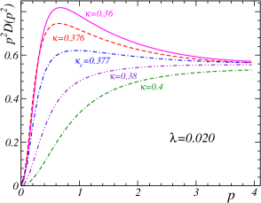
(a)	(b)

Figure 7: Momentum dependence of the fitted photon propagator form factor $D(p^{2})$ multiplied by $p^{2}$ for different $\kappa$’s near criticality for the first order (a) and continuous transition (b) regime.

we demonstrate how the momentum dependence of the propagator changes when crossing the first order or continuous transition. In the confinement region sufficiently away from the critical region the propagator form factor is practically the same irrespectively of the $\lambda$-value. Approaching the critical $\kappa_{c}$ from below, the form factor $p^{2}~{}D(p^{2})$ remains enhanced at intermediate momenta in the first order regime of small $\lambda$, changing then abruptly to a free massive propagator in the Higgs phase (deconfinement). Contrary to that, $p^{2}D(p^{2})$ varies continuously with increasing $\kappa$ crossing the (continuous) transition at the higher $\lambda$ value.

In order to demonstrate the influence of a less efficient gauge fixing procedure on the shape of the emerging photon propagator we show in Fig. 8

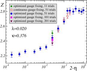
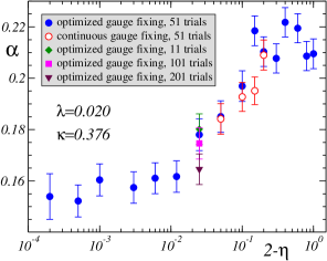
(a)	(b)

Figure 8: The fitted wave function normalization $Z$ (a) and anomalous dimension $\alpha$ (b) at $\lambda=0.02$ and $\kappa=0.376$ as functions of the overrelaxation parameter $\eta$.

the $\eta$ dependence of the fit parameters $Z$ and $\alpha$ on the confined side in the case of larger quartic Higgs self coupling obtained in 20 measurements. The dependence of the fit parameters resembles that of the gauge functional and the Dirac string density presented in Fig. 5 with a transition from a less ”perfect” level of performance to a better one around $2-\eta=10^{-1}...10^{-2}$. This strongly suggests that these fit parameters are closely related to the Dirac string density. We have checked that the minor discrepancy between the fit parameters at $\eta=1.85$ using the optimized and continuous gauge fixing goes away with increasing statistics.

In contrast to this, the other fit parameters $m$ and $C$ are roughly $\eta$ independent which points out that they depend only on the (gauge independent) monopole content. Still, a minor $\eta$ dependence of $Z$ and $\alpha$ might remain because we have used $\eta=1.997$ as a ”still affordable” choice. Probably a different gauge fixing algorithm has to be used to reduce this influence below the one-percent level. Comparing the obtained fitting results with those obtained earlier, with overrelaxation parameter $\eta=1.8$, for pure $U(1)$ CIS3 ; Chernodub:2002gp and for the Abelian Higgs model in the London limit Chernodub:2002en we have to admit that the presented numerical values for $Z$ and $\alpha$ in the confined phase are likely to reach values smaller by roughly 20 to 25 per cent once a better tuned $\eta$ is used. However, all qualitative results remain unchanged.

The resulting fit parameters near the first order transition are presented in Fig. 9 as functions of $\kappa$.

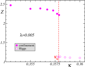
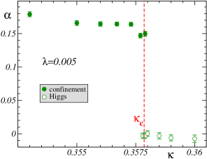
(a)	(b)
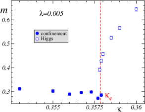
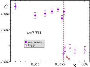
(c)	(d)

Figure 9: Fit parameters for the propagator at $\beta=2.0$ and $\lambda=0.005$ (in the first order transition region) as function of $\kappa$: (a) $Z$; (b) $\alpha$; (c) $m$; (d) $C$.

All parameters show a discontinuity at the phase transition. The metastability can be seen clearly reaching the transition from below (confined/symmetric phase) or from above (deconfined/Higgs phase). The anomalous dimension jumps from a non-zero positive value at low $\kappa$ to zero in the Higgs phase. The increasing mass of the photon propagator in the Higgs phase arises from the Higgs mechanism, whereas in the case of confinement the non-zero mass is due to the monopole plasma. Note that the mass is only very weakly dependent on $\kappa$ up to $\kappa_{c}$ in agreement with the behavior of the monopole density [compare Fig. 2(a)].

The corresponding results for the continuous transition regime are presented in Fig. 10.

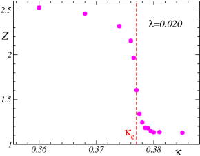
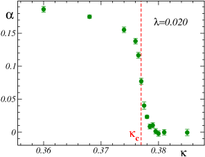
(a)	(b)
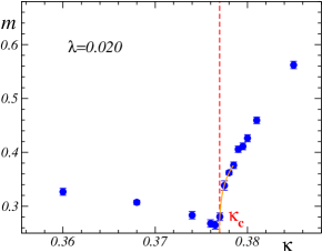
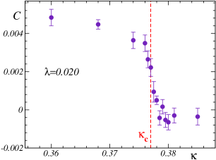
(c)	(d)

Figure 10: Fit parameters for the propagator at $\beta=2.0$ and $\lambda=0.02$ (in the continuous transition region) as function of $\kappa$: (a) $Z$; (b) $\alpha$; (c) $m$; (d) $C$. The fitted mass curve using Eq. (26) is indicated by the solid line in Fig. (c).

The fit parameters behave in complete analogy to the London limit: In the region very close to $\kappa_{c}$, the mass $m$ shows a minimum caused, as one could guess, by the interference between perturbative mass and Debye mass effects. Indeed, as $\kappa$ tends to $\kappa_{c}$, the Debye mass gets smaller since the density of the monopole-antimonopole plasma drops rapidly. One the other hand, the perturbative mass term becomes more significant. The interplay of these two tendencies results in the noticed minimum at $\kappa\approx\kappa_{c}$.

We have fitted the behavior of the mass parameter, $m$, as function of $\kappa$ on the Higgs side near the transition by the function

$$m(\kappa)=\mu{(\kappa-\kappa^{\mathrm{fit}}_{c})}^{\nu}\,,\qquad\kappa>\kappa_{c}\,.$$ (26)

The fit ansatz implies a vanishing mass at $\kappa_{c}$ what is actually not found numerically. So we treat that ansatz only phenomenologically. The best fit with $\chi^{2}/d.o.f.=1.3$ allows to determine $\kappa^{\mathrm{fit}}_{c}=0.3767(3)$, which agrees with the value from thermodynamic measurements given in Fig. 1(b) within errors. The estimated “critical exponent”, $\nu=0.19(6)$, differs from the mean field exponent, $\nu_{MF}=1/2$ which had been confirmed in Ref. ref:phase:prop1 ; ref:phase:prop2 for larger $\beta$. The fit including the four nearest fitted masses is shown in Fig. 10(c) by the solid line.

From the results for the anomalous dimension in both regimes we conclude that in cAHM with radial degrees of freedom the effect of the monopole pairing on the propagator is the same as in cQED: the anomalous dimension gets close to zero in the Higgs phase which is dominated by the magnetic dipole gas. This change is continuous in the continuous transition case (large $\lambda$), but discontinuous for the first order phase transition (small $\lambda$).

Similarly to the anomalous dimension, the effect of the monopole pairing on the renormalization parameter $Z$ of the photon wavefunction in cAHM, shown in Fig. 10(a), is remarkably similar to the cQED case observed in Refs. CIS3 ; Chernodub:2002gp . The wave function renormalisation $Z$ drops continuously across the continuous transition, but discontinuously at the first order transition for $\kappa$ reaching $\kappa_{c}$ from below.

V Conclusions

We have carefully investigated the problems afflicting the Landau gauge fixing procedure based on overrelaxation. An improved gauge fixing algorithm has been proposed and tested which uses a finite subgroup in a preselection/preconditioning stage. The computational gain in the expensive confinement region is a speed-up factor around ten. Such a stage could be useful for non-Abelian gauge groups as well.

We found that the gauge boson propagator of the three-dimensional compact Abelian Higgs model with radially active Higgs fields possesses a non-zero positive anomalous dimension in the confinement phase (at small $\kappa$). The momentum dependence of the propagator can be described by four parameters: the mass, the anomalous dimension, the photon renormalization function and the strength of the contact term.

At the first order phase transition (small Higgs self coupling) the parameters of the propagator show a discontinuity while in the vicinity of the continuous transition (large Higgs self coupling) the change of the parameters is continuous. Apart from the difference caused by the nature of the phase transition, the propagator behaves qualitatively similar to the propagator calculated in the London limit. Thus we conclude that the main ingredient which influences the gauge boson propagator is played by the compact phase of the Higgs field.

Note that the anomalous dimension of the gauge field does not become clearly negative neither in the confined phase nor in the deconfined phase. As it is found in the case of the cQED CIS3 ; Chernodub:2002gp the compactness of the gauge field provides a positive contribution to the anomalous dimension while the role Herbut ; AnomalousMatter of the dynamical Higgs fields is to make the anomalous dimension negative. Our study suggests that the positive contribution due to the compactness of the gauge fields is stronger than the negative contribution from the Higgs fields.

- (1) E. H. Fradkin and S. H. Shenker, Phys. Rev. D 19 (1979) 3682.
- (2) M. B. Einhorn and R. Savit, Phys. Rev. D 17 (1978) 2583; ibid. D 19 (1979) 1198.
- (3) H. Kleinert, F. S. Nogueira and A. Sudbø, Phys. Rev. Lett. 88 (2002) 232001; hep-th/0209132.
- (4) A. M. Polyakov, Nucl. Phys. B 120 (1977) 429.
- (5) M. N. Chernodub, E.-M. Ilgenfritz and A. Schiller, Phys. Lett. B 547 (2002) 269.
- (6) N. O. Agasian and D. Antonov, Phys. Lett. B 530 (2002) 153.
- (7) N. Parga, Phys. Lett. B 107 (1981) 442; N. O. Agasian and K. Zarembo, Phys. Rev. D 57 (1998) 2475.
- (8) M. N. Chernodub, E.-M. Ilgenfritz and A. Schiller, Phys. Rev. D 64 (2001) 054507; ibid. D 64 (2001) 114502.
- (9) M. N. Chernodub, E.-M. Ilgenfritz and A. Schiller, Phys. Rev. Lett. 88 (2002) 231601.
- (10) M. N. Chernodub, E. M. Ilgenfritz and A. Schiller, Phys. Rev. D 67 (2003) 034502.
- (11) M. N. Chernodub, E. M. Ilgenfritz and A. Schiller, hep-lat/0311033, to be published in Phys.Rev.D
- (12) K. Kajantie, M. Karjalainen, M. Laine and J. Peisa, Phys. Rev. B 57, 3011 (1998).
- (13) K. Kajantie, M. Karjalainen, M. Laine and J. Peisa, Nucl. Phys. B 520, 345 (1998).
- (14) V. P. Gerdt, A. S. Ilchev and V. K. Mitrjushkin, Yad. Fiz. 43, 736 (1986); A. Tarancon, Phys. Rev. D 36, 3211 (1987); K. Farakos, G. Koutsoumbas and S. Sarantakos, Z. Phys. C 40, 465 (1988).
- (15) G. Kohring, R. E. Shrock and P. Wills, Phys. Rev. Lett. 57 (1986) 1358.
- (16) M. N. Chernodub, E.-M. Ilgenfritz and A. Schiller, Phys. Lett. B 555 (2003) 206.
- (17) E.-M. Ilgenfritz, J. Kripfganz, H. Perlt and A. Schiller, Phys. Lett. B 356 (1995) 561.
- (18) M. Gürtler, E.-M. Ilgenfritz, J. Kripfganz, H. Perlt and A. Schiller, Nucl. Phys. B 483 (1997) 383.
- (19) M. Gürtler, E.-M. Ilgenfritz and A. Schiller, Phys. Rev. D 56 (1997) 3888.
- (20) S. Wenzel, Master thesis: “Monte Carlo simulations of the 3D Ginzburg-Landau model with compact U(1) gauge field ”, Leipzig university (2004)
- (21) R. Feldmann, diploma thesis, in preparation; M. N. Chernodub, R. Feldmann, E.-M. Ilgenfritz and A. Schiller, in preparation.
- (22) B. Bunk, Nucl. Phys. Proc. Suppl. 42 (1995) 566.
- (23) T. A. DeGrand and D. Toussaint, Phys. Rev. D 22 (1980) 2478.
- (24) V. G. Bornyakov, V. K. Mitrjushkin, M. Müller-Preussker and F. Pahl, Phys. Lett. B 317 (1993) 596.
- (25) P. Marenzoni, G. Martinelli and N. Stella, Nucl. Phys. B 455 (1995) 339; D. B. Leinweber, J. I. Skullerud, A. G. Williams and C. Parrinello, Phys. Rev. D 60 (1999) 094507; A. G. Williams, in Proc. of 3rd Int. Conf. on Quark Confinement and Hadron Spectrum, hep-ph/9809201; J. P. Ma, Mod. Phys. Lett. A 15 (2000) 229.
- (26) I. F. Herbut and Z. Tesanovic, Phys. Rev. Lett. 76 (1996) 4588.