Abstract

We study the temperature dependence of the monopole condensate in different Abelian projections of the $SU(2)$ lattice gauge theory. Using the Fröhlich-Marchetti monopole creation operator we show numerically that the monopole condensate depends on the choice of the Abelian projection. Contrary to the claims in the current literature we observe that in the Abelian Polyakov gauge and in the field strength gauge the monopole condensate does not vanish at the critical temperature and thus is not an order parameter.

1 Introduction

The confinement of color in QCD is one of the most interesting issues in the modern quantum field theory. Numerical simulations of non–Abelian gauge theories on the lattice [1] show that the confinement of quarks happens due to a formation of the chromoelectric strings spanned between quarks and anti-quarks. Although an analytical derivation of the color confinement is not available yet, there are various effective models which describe the emergence of the string. According to the dual superconductor model [2], the vacuum of a non–Abelian gauge model may be regarded as a medium of condensed Abelian monopoles. The monopole condensate squeezes the chromoelectric flux (coming from the quarks) into a flux tube due to the dual Meissner effect. This flux tube is an analogue of the Abrikosov vortex in an ordinary superconductor.

The basic element of the dual superconductor picture is the Abelian monopole. This object does not exist in QCD on the classical level, but is can be identified with a particular configuration of the gluon fields with the help of the so–called Abelian projection [3]. The Abelian projection uses a partial gauge fixing of the SU(N) gauge symmetry up to an Abelian subgroup. The compactness of the residual Abelian subgroup guarantees the existence of the Abelian monopoles in the Abelian projection.

Many numerical simulations show that the Abelian degrees of freedom in an Abelian projection are responsible for the confinement of quarks (for a review, see, $e.g.$, Refs. [4]). One of the striking features of the Abelian projection is the effect of the Abelian dominance [5]: the Abelian gauge fields provide a dominant contribution to the tension of the confining string. Moreover, the internal structure of the string energy, such as energy profile and the field distribution are very well described by the dual superconductor model [1].

Since qualitative features of the confinement mechanism in QCD and in the pure $SU(2)$ gauge theory are expected to be the same, below we restrict ourselves to the simplest case of the $SU(2)$ gluodynamics. Most of the results supporting the dual superconductor scenario were obtained in the so called Maximal Abelian (MA) projection [6]. According to numerical simulations [7, 8] the monopole condensate in the MA gauge is formed in the low temperature (confinement) phase and the condensate disappears in the high temperature (deconfinement) phase in the perfect agreement with the expectations coming from the dual superconductor scenario.

Besides the MA projection there are Abelian projections which are defined by a diagonalization of certain adjoint operators $X[U]$ with respect to the $SU(2)$ gauge transformations [3]. After the Abelian projection is fixed, the matrix $X[U]$ becomes diagonal and the theory possesses the (residual) $U(1)$ gauge symmetry. The most popular examples of such gauges are the Abelian Polyakov (AP) gauge and the Abelian field strength gauge ($F_{12}$ gauge). These gauges correspond, respectively, to the diagonalization of the Polyakov line and the $U_{12}$ plaquette variable.

One may ask whether a dual superconductor nature of non–Abelian vacuum is realized in all Abelian gauges. Needless to say that this question is important for understanding of the properties of the QCD vacuum. Indeed, it seems natural that the color confinement must be described by a projection–independent model since the confinement is a gauge invariant phenomenon. On the other hand one can consider the Abelian projection as a gauge–dependent tool to associate the confining gluon configurations with the Abelian monopoles. This tool may work well in one gauge and may not work in another gauge.

There are conflicting reports of the projection independence of the dual superconductor mechanism of the color confinement. The Abelian and Monopole dominance were observed in more than one gauge [5, 10]. The London penetration length measured in the MA projection is the same as the one obtained without gauge fixing [11]. The monopole condensation studied with the help of a monopole creation operator was observed not only in the MA gauge of $SU(2)$ gauge theory [7, 8] but also in other gauges [12].

On the other hand there are indications that the monopole dynamics is affected by the choice of the Abelian projection. In the MA gauge the monopole trajectories percolate only in the confinement phase contrary to the case without any gauge fixing, in which the monopoles are percolating in any phase [13]. The chromoelectric string in different Abelian projections looks differently: the correlation length (the inverse monopole mass) extracted from the string profile in the AP gauge is consistent with zero contrary to the MA gauge [14]. The chiral condensate is dominated by the contributions of the Abelian monopoles in the MA gauge [15, 16] contrary to $F_{12}$ [15] and AP [16] gauges.

One can show analytically that in the AP gauge the dual superconductor mechanism can not be realized [9]. The reason is very simple: the monopoles in the continuum limit in this gauge are static and they can not contribute to the potential between static heavy quarks. On the other hand it was shown in Ref. [9] that the absence of the dual superconductor description in AP gauge does not contradict to the statement of Ref. [12] that the monopole condensation is realized in any gauge.

In this paper we are studying the effective potential for the monopole field using the Fröhlich-Marchetti [17] monopole creation operator. We evaluate the potential in AP and $F_{12}$ gauges and compare the results with the monopole potential obtained in the MA gauge [7]. The value of the monopole condensate is defined by the minimum of the effective potential. We describe the monopole creation operator in Section 2 and present numerical results in Section 3. Our conclusions are summarized in the last Section.

2 Abelian monopole creation operator in SU(2) model

We study the $SU(2)$ gauge theory with the standard Wilson action, $S[U]=-1/2\sum_{P}\mbox{Tr}\,U_{P}$, where the sum goes over the plaquettes $P$ and $U_{P}$ is the $SU(2)$ plaquette variable composed of the link fields $U_{l}$, $U_{P}=U_{1}U_{2}U_{3}^{\dagger}U_{4}^{\dagger}$. The link field is parameterized in the standard way:

$$U_{x\mu}=\left(\begin{array}[]{ll}\cos\phi_{x\mu}\,e^{i\theta_{x\mu}}&\sin\phi_{x\mu}\,e^{i\chi_{x\mu}}\\ -\sin\phi_{x\mu}\,e^{-i\chi_{x\mu}}&\cos\phi_{x\mu}\,e^{i\theta_{x\mu}}\\ \end{array}\right)\,,$$ (3)

$0\leq\phi\leq\pi/2$ and $-\pi<\theta,\chi\leq\pi$.

In Abelian projection the residual gauge transformation matrices have the diagonal form $\Omega^{\mathrm{Abel}}(\omega)={\mathrm{diag}(e^{i\omega},e^{-i\omega})}$, where $\omega$ is an arbitrary scalar function. Under these transformations the diagonal field $\theta$ transforms as an Abelian gauge field, $\theta_{x\mu}\to\theta_{x\mu}+\omega_{x}-\omega_{x+\hat{\mu}}$, the off-diagonal field $\chi$ changes as a double charged matter field, $\chi_{x\mu}\to\chi_{x\mu}+\omega_{x}+\omega_{x+\hat{\mu}}$, the field $\phi$ remains intact. The $SU(2)$ plaquette action contains [18] various interactions between these fields as well as the action for the Abelian gauge field $\theta$:

$$S[U]=-\sum_{P}\beta_{P}[\phi]\cos\theta_{P}+\dots\,.$$ (4)

Here $\theta_{P}=\theta_{1}+\theta_{2}-\theta_{3}-\theta_{4}$ is a lattice analogue of the Abelian field strength tensor and $\beta_{P}[\phi]$ is an effective coupling constant dependent of the fields $\phi$, Ref. [18].

Following Ref. [7] we apply the monopole creation operator of Fröhlich-Marchetti [17] to the Abelian part of the non–Abelian action (4). Effectively, this operator shifts the Abelian plaquette variable $\theta_{P}$ as follows:

$$\Phi_{mon}(x)=\exp\left\{\sum_{P}\beta_{P}[\phi]\biggl{[}-\cos\theta_{P}+\cos(\theta_{P}+W_{P}(x))\biggr{]}\right\}\,,$$ (5)

where $W_{P}=2\pi\delta\Delta^{-1}(D_{x}-\omega_{x})$, $\omega_{x}$ is a Dirac string attached to the monopole and the Dirac cloud $D_{x}$ satisfies the equation $\delta{}^{*}{D}_{x}={}^{*}{\delta}_{x}$.

We have used the differential form notations on the lattice described in detail in the second paper in Ref. [4]. $\delta$ ($\mathrm{d}$) is the backward (forward) derivative on the lattice which decreases (increases) by one the rank of the form on which it acts. The rank of the form is determined by a dimensionality of the lattice cell on which this form is defined. For example, a scalar function is a 0-form, the vector function is a 1-form etc. If $A$ is a lattice vector, then $\delta A$ is a scalar (a lattice analogue of the divergence, $\partial_{\mu}A_{\mu}$) while $\mathrm{d}A$ is an antisymmetric tensor (a lattice analogue of the field strength, $\partial_{[\mu,}A_{\nu]}$). $\delta$ and $\mathrm{d}$ operators are nilponent, i.e., $\delta^{2}=0=\mathrm{d}^{2}$. The lattice Laplacian is $\Delta=\delta\mathrm{d}+\mathrm{d}\delta$, and $\Delta^{-1}$ is the inverse Laplacian. The lattice Kronecker symbol is denoted as $\delta_{x}$: it is a scalar function which is equal to unity at the site $x$ and zero otherwise. The *-operator relates the forms on the dual and original lattice. For example, if on the four-dimensional lattice $B$ is a scalar function (0-form) on the original lattice, then ${}^{*}{B}$ is a 4-form on the dual lattice.

The operator (5) is clearly gauge invariant with respect to the $U(1)$ gauge transformations. One can also perform a formal duality transformation with respect to the quantum average of the operator (5) and show that in the dual model – which has form of the Abelian Higgs model – this operator is invariant under the (dual) gauge transformations [7]. Moreover, one can represent the partition function as a sum over closed monopole trajectories. In this representation the quantum average of the monopole creation operator $\Phi_{mon}(x)$, Eq. (5), is given by a sum over all closed monopole trajectories plus one open trajectory which begins at the point $x$, Refs. [17]. Thus, this operator creates a monopole at the point $x$.

To get the monopole condensate we have to study the effective constraint potential for the monopole creation operator $\Phi_{mon}$,

$$V_{effc}(\Phi)=-\ln(\langle\delta(\Phi-\frac{1}{V}\sum_{x}\Phi_{mon}(x))\rangle)\,.$$ (6)

This potential selects the zero–momentum component of the creation operator. The minimum of this potential corresponds to the monopole condensate. However, a numerical calculation of the potential $V_{effc}(\Phi)$ is time consuming, and in this paper we present results for the probability distribution

$$V(\Phi)=-\ln(\langle\delta(\Phi-\Phi_{mon}(x))\rangle)\,,$$ (7)

which has a meaning very similar to (6).

We perform our study in the Abelian Polyakov gauge and in the Abelian field strength gauge which are defined as we already discussed by the diagonalization of the (untraced) Polyakov loop, $P_{x}[U]$, and of the $U_{x,12}$ plaquette,

$$P_{x}[U]=U_{x,4}U_{x+\hat{4},4}\dots U_{x-\hat{4},4}\,,\quad U_{x,12}=U_{x,1}U_{x+\hat{1},2}U^{\dagger}_{x+\hat{2},1}U^{\dagger}_{x,2}\,,$$ (8)

with respect to gauge transformations, $U_{x,\mu}\to\Omega_{x}U_{x,\mu}\Omega^{\dagger}_{x+\hat{\mu}}$.

We compare the potential in these gauges with the monopole potential obtained in the MA gauge in Ref. [7]. The MA gauge is defined by the maximization of the lattice functional

$$\max_{\Omega}R_{MA}[U^{\Omega}]\,,\qquad R_{MA}[U]=\sum_{s,\hat{\mu}}{\rm Tr}\Big{(}\sigma_{3}U(s,\mu)\sigma_{3}U^{\dagger}(s,\mu)\Big{)}\,.$$ (9)

($\sigma_{3}$ is the Pauli matrix). In the continuum limit a local condition of the maximization can be written in the form of the differential equation, $(\partial_{\mu}+igA_{\mu}^{3})(A_{\mu}^{1}-iA_{\mu}^{2})=0$.

3 Numerical results

We simulate the $SU(2)$ gauge fields on the lattices $L_{s}^{3}\times 4$, $L_{s}=12,14,16,24$ with $C$–periodic boundary conditions in space directions [21]. The $C$–periodicity corresponds to the anti-periodicity for the Abelian gauge fields which is required by the Gauss law [7]. In the case of $SU(2)$ gauge group the $C$–periodic boundary conditions mean that on the space boundary we have $U_{x,\mu}\to\Omega^{+}U_{x,\mu}\Omega,\,\,\Omega=i\sigma_{2}$.

We fix AP and $F_{12}$ gauges as it was described in the previous Section. The results for the MA gauge (quoted below) are taken from Ref. [7]. To get the effective potential in the AP and $F_{12}$ gauges we use 400 independent configurations of $SU(2)$ gauge fields for each value of the gauge coupling $\beta$ at a given lattice volume. On each configuration the distribution of the monopole creation operator is evaluated in 20 points. The logarithm of the distribution provides us with the effective potential (7).

To evaluate the numerical errors of the potential we use the bootstrap method. For each value of $\beta$ and the lattice volume we get a distribution of the values of the monopole creation operator (”initial ensemble”). Then we use the initial ensemble to construct a number (typically $N_{ens}=500$) of additional ensembles of the operator values by randomly choosing the entries from the initial ensemble. Each value from the initial ensemble may enter the additional ensemble more than one time. The number of entries in each of the additional ensembles is the same as in the initial one. Then for each ensemble we construct a histogram, the (minus) logarithm of which has a meaning of the monopole potential, $V(\Phi)$, according to Eq. (7). Thus, for each value of the monopole field, $\Phi$, we get $N_{ens}$ values of the potential, $V$, which form a Gaussian distribution. The central value of this distribution gives us the value of the potential at given lattice volume $L_{s}^{2}\times L_{t}$, $\beta$ and $\Phi$, $V=V(\Phi)$, while the width of the distribution is the statistical error.

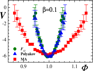
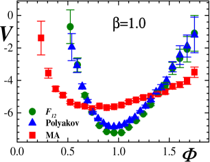
(a)	(b)
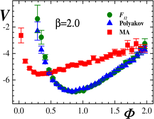
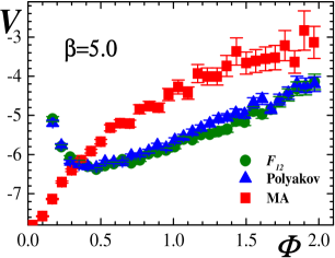
(c)	(d)

Figure 1: The potential on the monopole field in the MA, AP and $F_{12}$ gauges at various values of the gauge coupling $\beta$. The data for the MA gauge are taken from Ref. [7].

The examples of the effective monopole potentials for $16^{3}\times 4$ lattice are shown on Figs. 1(a-d). We depict the positive part of the potentials ($\Phi>0$) at various values of the gauge coupling $\beta$ in the MA, AP and $F_{12}$ gauges. The minimum of the effective potential corresponds to the value of the monopole condensate. The critical gauge coupling corresponding to the temperature phase transition at our lattices is $\beta_{c}\approx 2.3$. Thus Figs. 1(a,b,c) correspond to the confinement phase while Fig. 1(d) corresponds to the deconfinement phase.

First of all we note that for all considered values of $\beta$ (i) the minima of the potentials in the AP and $F_{12}$ gauges coincide with each other within numerical errors; (ii) the potential in the MA gauge is different from AP and $F_{12}$ potentials. According to Fig. 1(a) in the strong coupling limit ($\beta=0.1$) the minima of the monopole potential in all three gauges are located at the same point, $\Phi_{\min}\approx 1$. As we increase $\beta$ the difference in the monopole condensates in MA gauge and in AP and $F_{12}$ gauges appears, see Fig. 1(b,c). Moreover, in the deep deconfinement phase, Fig. 1(d), the monopole condensate vanishes in MA gauge while in AP and $F_{12}$ gauges the condensate is non–zero.

Since the phase transition in the $SU(2)$ gauge theory is of the second order, the finite volume effects may be essential for the determination of the monopole condensate. To get rid of finite volume corrections we measure the condensate on the lattices with various spatial extensions ($L_{s}=12,14,16,24$) and extrapolate the value of the condensate to the thermodynamic limit, $L_{s}\to\infty$:

$$\Phi_{c}=\Phi^{\mathrm{inf}}_{c}+\frac{C}{L}\,.$$ (10)

The examples of the fits for the AP and the $F_{12}$ gauges are shown in Figs. 2(a,b). The values of $\chi^{2}/d.o.f.$ are in the range $0.2\sim 1$.

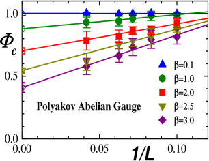
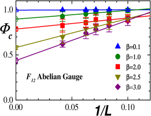
(a)	(b)

Figure 2: The extrapolation (10) of the monopole condensate to the thermodynamic limit in the AP and the $F_{12}$ gauges for various values of the gauge coupling $\beta$. The spatial extensions of the lattices are $L_{s}=12,14,16,24$.

The monopole condensates in the thermodynamic limit ($L_{s}\to\infty$) for all three Abelian projections are shown in Fig. 3 as functions of $\beta$. One can clearly see that the monopole condensate in the MA projection vanishes at a certain critical $\beta=\beta_{c}$ which is very close to the phase transition point, $\beta_{c}\approx 2.3$. Contrary to the MA gauge the monopole condensates obtained in the AP and the $F_{12}$ gauges do not vanish at $\beta=\beta_{c}$. This result is in contradiction with observations of Ref. [12].

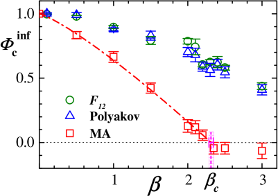
Figure 3: The monopole condensate in the thermodynamic limit in the MA, the AP and the $F_{12}$ gauges. The dash–dotted line is the fit of the monopole condensate in the MA gauge by Eq. (11). The critical value of the gauge coupling (along with the numerical error) is denoted by the vertical dashed line.

The dependence of the monopole condensate on $\beta$ can be fitted by the following function:

$$\Phi^{\mathrm{inf}}_{c}(\beta)=1-(\beta/\beta_{c})^{\gamma}\,,$$ (11)

with $\chi^{2}/d.o.f.\approx 0.3$. It occurs that $\gamma=1.2(5)$ and $\beta_{c}=2.31(3)$. The value of $\beta_{c}$ coincides within error bars with the known critical value [22] on $L_{s}^{3}\times 4$ lattice.

4 Conclusion

Summarizing, we have presented an evidence that the monopole condensate in different Abelian projections coincide with each other only in the (unphysical) strong coupling region. Generally, the condensate depends on the choice of the Abelian projection. We have considered three Abelian projections and only in MA projection the vacuum behaves as the dual superconductor. Our results are in contradiction with conclusions of Ref. [12] where condensate was found to be projection–independent.

References

- [1] V. Singh, D. A. Browne, R. W. Haymaker, Phys. Lett. B 306, 115 (1993); G. S. Bali, K. Schilling, C. Schlichter, Phys. Rev. D 51, 5165 (1995); G. S. Bali, C. Schlichter, K. Schilling, Prog. Theor. Phys. Suppl. 131, 645 (1998); F. V. Gubarev, E. M. Ilgenfritz, M. I. Polikarpov, T. Suzuki, Phys. Lett. B 468, 134 (1999); Y. Koma, M. Koma, E. M. Ilgenfritz, T. Suzuki and M. I. Polikarpov, Phys. Rev. D 68, 094018 (2003); Y. Koma, M. Koma, E. M. Ilgenfritz and T. Suzuki, Phys. Rev. D 68, 114504 (2003).
- [2] G. ’t Hooft, in High Energy Physics, ed. A. Zichichi, EPS International Conference, Palermo (1975); S. Mandelstam, Phys. Rept. 23, 245 (1976).
- [3] G. ’t Hooft, Nucl. Phys. B190, 455 (1981).
- [4] T. Suzuki, Nucl. Phys. Proc. Suppl. 30, 176 (1993); M. N. Chernodub, M. I. Polikarpov, “Abelian projections and monopoles”, in ”Confinement, duality, and nonperturbative aspects of QCD”, Ed. by P. van Baal, Plenum Press, p. 387, hep-th/9710205; R.W. Haymaker, Phys. Rept. 315, 153 (1999).
- [5] T. Suzuki, I. Yotsuyanagi, Phys. Rev. D42, 4257 (1990); H. Shiba, T. Suzuki, Phys. Lett. B 333, 461 (1994); G. S. Bali, V. Bornyakov, M. Müller-Preussker, K. Schilling, Phys. Rev. D54, 2863 (1996).
- [6] A. S. Kronfeld, M. L. Laursen, G. Schierholz, U. J. Wiese, Phys. Lett. B 198, 516 (1987); A. S. Kronfeld, G. Schierholz, U. J. Wiese, Nucl. Phys. B 293, 461 (1987).
- [7] M. N. Chernodub, M. I. Polikarpov, A. I. Veselov, Phys. Lett. B 399, 267 (1997); Nucl. Phys. Proc. Suppl. 49, 307 (1996);
- [8] A. Di Giacomo, G. Paffuti, Phys. Rev. D 56, 6816 (1997).
- [9] M. N. Chernodub, “Monopoles in Abelian Polyakov gauge and projection (in)dependence of the dual superconductor mechanism of confinement”, hep-lat/0308031.
- [10] J. D. Stack, S. D. Neiman, R. J. Wensley, Phys. Rev. D 50, 3399 (1994); Y. Matsubara, S. Ilyar, T. Okude, K. Yotsuji and T. Suzuki, Nucl. Phys. Proc. Suppl. 42, 529 (1995); S. Ejiri, S. I. Kitahara, Y. Matsubara, T. Okude, T. Suzuki, K. Yasuta, Nucl. Phys. Proc. Suppl. 47, 322 (1996); A. J. van der Sijs, Nucl. Phys. Proc. Suppl. 73, 548 (1999); S. Fujimoto, S. Kato, T. Suzuki and T. Tsunemi, Prog. Theor. Phys. Suppl. 138, 36 (2000).
- [11] P. Cea, L. Cosmai, Phys. Lett. B 349, 343 (1995).
- [12] A. Di Giacomo, B. Lucini, L. Montesi, G. Paffuti, Phys. Rev. D 61, 034503 (2000); ibid., 034504 (2000).
- [13] A.I. Veselov and M.A. Zubkov, unpublished (1998).
- [14] K. Bernstein, G. Di Cecio, R. W. Haymaker, Phys. Rev. D 55, 6730 (1997).
- [15] R. M. Woloshyn, Phys. Rev. D 51, 6411 (1995).
- [16] F. X. Lee, R. M. Woloshyn, H. D. Trottier, Phys. Rev. D 53, 1532 (1996).
- [17] J. Fröhlich and P.A. Marchetti, Commun. Math. Phys., 112 (1987) 343.
- [18] M. N. Chernodub, M. I. Polikarpov, A. I. Veselov, Phys. Lett. B 342, 303 (1995).
- [19] J. Frohlich and P. A. Marchetti, Phys. Rev. D 64, 014505 (2001).
- [20] V. A. Belavin, M. N. Chernodub and M. I. Polikarpov, Phys. Lett. B 554, 146 (2003); JETP Lett. 75, 217 (2002) [Pisma Zh. Eksp. Teor. Fiz. 75, 263 (2002)].
- [21] U.J. Wiese, Nucl.Phys. B375, 45 (1992).
- [22] J. Engels, J. Fingberg and M. Weber, Nucl. Phys. B 332 737 (1990).