INT-PUB 04-05

NT@UW-04-03

UW/PT 04-02

Heavy meson chiral perturbation theory in finite volume

Daniel Arndt^a and C.-J. David Lin^a,b
a Department of Physics, University of Washington, Seattle, WA 98195-1560, USA.
^b Institute for Nuclear Theory, University of Washington, Seattle, WA 98195-1550, USA.

Abstract:
We study finite volume effects in heavy quark systems in the framework of heavy meson chiral perturbation theory for full, quenched, and partially quenched QCD. A novel feature of this investigation is the role played by the scales $\Delta_{\ast}$ and ${\delta}_{s}$, where $\Delta_{\ast}$ is the mass difference between the heavy-light vector and pseudoscalar mesons of the same quark content, and ${\delta}_{s}$ is the mass difference due to light flavour $SU(3)$ breaking. The primary conclusion of this work is that finite volume effects arising from the propagation of Goldstone particles in the effective theory can be altered by the presence of these scales. Since $\Delta_{\ast}$ varies significantly with the heavy quark mass, these volume effects can be amplified in both heavy and light quark mass extrapolations (interpolations). As an explicit example, we present results for $B$ parameters of neutral $B$ meson mixing matrix elements and heavy-light decay constants to one-loop order in finite volume heavy meson chiral perturbation theory for full, quenched, and $N_{f}=2+1$ partially quenched QCD. Our calculation shows that for high-precision determinations of the phenomenologically interesting $SU(3)$ breaking ratios, finite volume effects are significant in quenched and not negligible in partially quenched QCD, although they are generally small in full QCD.

PACS numbers: 11.15.Ha,12.38.Gc,12.15Ff

I Introduction

Numerical calculations of hadronic properties using lattice QCD have provided significant inputs to particle physics phenomenology. In particular, the joint effort between experiment and theory to investigate the unitarity triangle in the Cabibbo-Kobayashi-Maskawa (CKM) matrix from $B$ meson decays and mixing has made impressive progress Battaglia:2003in , in which lattice QCD has played an important role. Nevertheless, current lattice calculations are still subject to various systematic errors. In this paper, we address finite volume effects which arise in lattice calculations for heavy-light meson systems from the light degrees of freedom. Our framework is heavy meson chiral perturbation theory (HM$\chi$PT) with first order $1/M_{P}$ and chiral corrections. We assume the mass hierarchy

$$M_{\mathrm{GP}}\ll\Lambda_{\chi}\ll M_{P},$$ (1)

where $M_{\mathrm{GP}}$ is the mass of any Goldstone particle, $M_{P}$ is the mass of the heavy-light meson, and $\Lambda_{\chi}$ is the chiral symmetry breaking scale. Under this assumption, we discard corrections of the size

$$\frac{M_{\mathrm{GP}}}{M_{P}}.$$ (2)

Concerning the finite volume, we work with the condition that

$$M_{\mathrm{GP}}L\gg 1,$$ (3)

where $L$ is the spatial extent of the cubic box. Therefore, given that $f_{\pi}L/\sqrt{2}$ ($f_{\pi}\approx 132\mbox{ MeV}$) will be close to one in lattice simulations in the near future, one can still neglect the chiral symmetry restoration effects resulting from the Goldstone zero momentum modes Gasser:1987ah ; Leutwyler:1992yt when Eq. (3) is satisfied.

The main task of this work is to study the volume effects due to the presence of the scales

$$\Delta_{\ast}=M_{P^{\ast}}-M_{P},$$ (4)

and

$$\delta_{s}=M_{P_{s}}-M_{P},$$ (5)

where $P^{\ast}$ and $P$ are the heavy-light vector and pseudoscalar mesons containing a $u$ or $d$ anti-quark, and $P_{s}$ is the heavy-light pseudoscalar meson with an $s$ anti-quark. The scale $\Delta_{\ast}$ appears due to the breaking of heavy quark spin symmetry that is of ${\mathcal{O}}(1/M_{P})$ and $\delta_{s}$ comes from light flavour $SU(3)$ breaking in the heavy-light meson masses. Under the assumption of Eq. (1), $\Delta_{\ast}$ is independent of the light quark mass, and $\delta_{s}$ does not contain any $1/M_{P}$ corrections, at the order we are working.

In the real world, both $\Delta_{\ast}$ and $\delta_{s}$ are not very different from the pion mass. In fact Hagiwara:2002fs ,

$$M_{B_{s}}-M_{B}=91\mbox{ MeV},$$ (6)

$$M_{D_{s}}-M_{D}=104\mbox{ MeV},$$ (7)

$$M_{B^{\ast}}-M_{B}=46\mbox{ MeV},$$ (8)

and

$$M_{D^{\ast}}-M_{D}=142\mbox{ MeV}.$$ (9)

In current lattice simulations, these mass splittings vary between 0 and $\sim 150$ MeV. Therefore it is important to include them in the investigation of finite volume effects. Equation (3) implies that the Compton wavelength of the Goldstone particle is small compared to the size of the box. Therefore finite volume effects mainly result from the propagation of the Goldstone particles to the boundary. However, as shown in Section III, $\Delta_{\ast}$ and $\delta_{s}$ can, in a non-trivial way, alter these effects. In particular, since $\Delta_{\ast}$ varies with the heavy quark mass, finite volume effects can be significantly amplified in heavy quark mass extrapolations.

This paper is organised as follows. In Section II we summarise the ingredients of HM$\chi$PT relevant to this work. Section III is devoted to the discussion of HM$\chi$PT in finite volume, emphasising the role played by $\delta_{s}$ and $\Delta_{\ast}$. We then present an explicit calculation of neutral $B$ meson mixing and heavy-light decay constants in Section IV and discuss the phenomenological impact that finite volume effects can have. We conclude in Section V. Some mathematical formulae and results are summarised in the appendices.

As this work progressed, we were informed that similar ideas and techniques were also being applied in heavy baryon chiral perturbation theory beane:to_appear . Although the underlying physics is somewhat different, many technical aspects are quite similar to those presented here.

II Heavy meson chiral perturbation theory

The chiral Lagrangian for the Goldstone particles is

$${\mathcal{L}}_{\mathrm{GP}} = \frac{f^{2}}{8}{\mathrm{(s)tr}}\left[\big{(}\partial_{\mu}\Sigma^{\dagger}\big{)}\big{(}\partial^{\mu}\Sigma\big{)}+\Sigma^{\dagger}\chi+\chi^{\dagger}\Sigma\right]$$ (10)

$$+A_{\eta^{\prime}}\left[\alpha(\partial_{\mu}\Phi_{0})(\partial^{\mu}\Phi_{0})-M_{0}^{2}\Phi^{2}_{0}\right],$$

where $A_{\eta^{\prime}}=1$ for quenched QCD (QQCD) and partially quenched QCD (PQQCD), and $A_{\eta^{\prime}}=0$ for full QCD. $\Sigma={\mathrm{exp}}(2i\Phi/f)$ is the non-linear Goldstone particle field, with $\Phi$ being the matrix containing the standard Goldstone fields. We use $f=132$ MeV. In this work, we follow the supersymmetric formulation of (partially) quenched chiral perturbation theory [(P)Q$\chi$PT] Bernard:1992mk ; Bernard:1994sv . Therefore $\Sigma$ transforms linearly under $SU(3)_{\mathrm{L}}\otimes SU(3)_{\mathrm{R}}$, $SU(3|3)_{\mathrm{L}}\otimes SU(3|3)_{\mathrm{R}}$ and $SU(6|3)_{\mathrm{L}}\otimes SU(6|3)_{\mathrm{R}}$ in full QCD, QQCD and PQQCD respectively. The symbol “(s)tr” in the above equation means “trace” in full QCD and “supertrace” in (P)QQCD. The variable $\chi$ is defined as

$$\chi\equiv 2B_{0}{\mathcal{M}}_{q}=\frac{-2\langle 0|\bar{u}u+\bar{d}d|0\rangle}{f^{2}}{\mathcal{M}}_{q},$$ (11)

where the quark mass matrix ${\mathcal{M}}_{q}$ is

$${\mathcal{M}}^{\mathrm{(QCD)}}_{q}={\mathrm{diag}}(m,m,m_{s}),$$ (12)

in full QCD,

$${\mathcal{M}}^{({\mathrm{QQCD}})}_{q}={\mathrm{diag}}(\underbrace{m,m,m_{s}}_{{\mathrm{valence}}},\underbrace{m,m,m_{s}}_{{\mathrm{ghost}}}),$$ (13)

in QQCD, and

$${\mathcal{M}}^{({\mathrm{PQQCD}})}_{q}={\mathrm{diag}}(\underbrace{m,m,m_{s}}_{{\mathrm{valence}}},\underbrace{\tilde{m},\tilde{m},\tilde{m}_{s}}_{{\mathrm{sea}}},\underbrace{m,m,m_{s}}_{{\mathrm{ghost}}}),$$ (14)

in PQQCD. We keep the strange quark mass different from that of the up and down quarks in the valence, sea and ghost sectors. Notice that the flavour singlet state $\Phi_{0}={\mathrm{str}}(\Phi)/\sqrt{6}$ is rendered heavy by the $U(1)_{A}$ anomaly in PQQCD Sharpe:2001fh ; Sharpe:2000bc and can be integrated out; it has to be kept as a dynamical degree of freedom in QQCD.

The inclusion of the heavy-light mesons in chiral perturbation theory (HM$\chi$PT) was first proposed in Refs. Burdman:1992gh ; Wise:1992hn ; Yan:1992gz , with the generalisation to quenched and partially quenched theories given in Refs. Booth:1995hx ; Sharpe:1996qp . The $1/M_{P}$ and chiral corrections were studied by Boyd and Grinstein Boyd:1995pa in full QCD and by Booth Booth:1994rr in QQCD. The spinor field appearing in this effective theory is

$$H^{(Q)}_{a}=\frac{1+/\!\!\!v}{2}\left(P^{\ast(Q)}_{a,\mu}\gamma^{\mu}-P^{(Q)}_{a}\gamma_{5}\right),$$ (15)

where $P^{(Q)}_{a}$ and $P^{\ast(Q)}_{a,\mu}$ annihilate pseudoscalar and vector mesons containing a heavy quark $Q$ and a light anti-quark of flavour $a$. Under a heavy quark spin $SU(2)$ transformation $S$,

$$H^{(Q)}_{a}\longrightarrow SH^{(Q)}_{a}.$$ (16)

Under the vector light-flavour transformation $U$ [i.e., $U\in SU(3)$ for full QCD, $U\in SU(3|3)$ for QQCD and $U\in SU(6|3)$ for PQQCD],

$$H^{(Q)}_{a}\longrightarrow H^{(Q)}_{b}U^{\dagger}_{ba}.$$ (17)

Also, the conjugate field, which creates heavy-light mesons containing a heavy quark $Q$ and a light anti-quark of flavour $a$, is defined as

$$\bar{H}^{(Q)}_{a}=\gamma^{0}H^{(Q)}\gamma_{0}.$$ (18)

Furthermore, the Goldstone particles appear in the HM$\chi$PT Lagrangian via the field

$$\xi\equiv{\mathrm{e}}^{i\Phi/f},$$ (19)

which transforms as

$$\xi\longrightarrow U_{\mathrm{L}}\xi U^{\dagger}=U\xi U^{\dagger}_{\mathrm{R}},$$ (20)

where $U_{\mathrm{L(R)}}$ is an element of the left-handed (right-handed) $SU(3)$, $SU(3|3)$ and $SU(6|3)$ groups for QCD, QQCD, and PQQCD respectively. The HM$\chi$PT Lagrangian, to lowest order in the chiral and $1/M_{Q}$ expansion, for mesons containing a heavy quark $Q$ and a light anti-quark of flavour $a$ is then

$${\mathcal{L}}_{\mathrm{HM\chi PT}} = -i\,{\mathrm{tr_{D}}}\left(\bar{H}^{(Q)}_{a}v_{\mu}\partial^{\mu}H^{(Q)}_{a}\right)+\frac{i}{2}{\mathrm{tr_{D}}}\left(\bar{H}^{(Q)}_{a}v_{\mu}\left[\xi^{\dagger}\partial^{\mu}\xi+\xi\partial^{\mu}\xi^{\dagger}\right]_{ab}H^{(Q)}_{b}\right)$$

$$+\frac{i}{2}g\,{\mathrm{tr_{D}}}\left(\bar{H}^{(Q)}_{a}\gamma_{\mu}\gamma_{5}\left[\xi^{\dagger}\partial^{\mu}\xi-\xi\partial^{\mu}\xi^{\dagger}\right]_{ab}H^{(Q)}_{b}\right)+B_{\eta^{\prime}}\frac{i}{2}\gamma\,{\mathrm{tr_{D}}}\left(\bar{H}^{(Q)}_{a}H^{(Q)}_{a}\gamma_{\mu}\gamma_{5}\right){\mathrm{str}}\left[\xi^{\dagger}\partial^{\mu}\xi-\xi\partial^{\mu}\xi^{\dagger}\right],$$

where $B_{\eta^{\prime}}=0$ for full QCD, and $B_{\eta^{\prime}}=1$ for (P)QQCD. We do not distinguish the coupling $g$ in these theories. It is implicitly assumed that “${\mathrm{(s)tr}}_{a}$” is taken appropriately in flavour space. ${\mathrm{tr_{D}}}$ means taking the trace in Dirac space. The HM$\chi$PT Lagrangian for mesons containing a heavy anti-quark $\bar{Q}$ and a light quark of flavour $a$ is obtained by applying the charge conjugation operation to the above Lagrangian Grinstein:1992qt . At this order, the propagators for $P^{(Q)}_{a}$ and $P^{\ast(Q)}_{a}$ mesons are

$$\frac{i}{2(v\cdot k+i\epsilon)}\mbox{ },\mbox{ }\mbox{ }\frac{-i(g_{\mu\nu}-v_{\mu}v_{\nu})}{2(v\cdot k+i\epsilon)},$$ (22)

respectively.

The effects of chiral and heavy quark symmetry breaking have been systematically studied in full Boyd:1995pa and quenched Booth:1994rr HM$\chi$PT. Amongst them, the only relevant feature necessary for the purpose of this work, i.e., the investigation of finite volume effects, are the shifts to the masses of the heavy-light mesons. These shifts are from the heavy quark spin breaking term

$$\frac{\lambda_{2}}{M_{P}}{\mathrm{tr_{D}}}\left(\bar{H}^{(Q)}_{a}\sigma_{\mu\nu}H^{(Q)}_{a}\sigma^{\mu\nu}\right),$$ (23)

and the chiral symmetry breaking terms

$$\lambda_{1}B_{0}\mbox{ }{\mathrm{tr_{D}}}\left(\bar{H}^{(Q)}_{a}\left[\xi{\mathcal{M}}_{q}\xi+\xi^{\dagger}{\mathcal{M}}_{q}\xi^{\dagger}\right]_{ab}H^{(Q)}_{b}\right)$$

$$+\lambda_{1}^{\prime}B_{0}\mbox{ }{\mathrm{tr_{D}}}\left(\bar{H}^{(Q)}_{a}H^{(Q)}_{a}\right)\left[\xi{\mathcal{M}}_{q}\xi+\xi^{\dagger}{\mathcal{M}}_{q}\xi^{\dagger}\right]_{bb}.$$

We choose to work with the effective theory in which the heavy-light pseudoscalar mesons that contain a heavy quark and a $u$ or $d$ valence anti-quark are massless. Notice that the term proportional to $\lambda^{\prime}_{1}$ in Eq. (II) causes a universal shift to all the heavy-light meson masses. This means that the masses appearing in the propagators of heavy vector mesons and any meson containing an $s$ anti-quark (valence or ghost) are shifted as follows:

$$\frac{-i(g_{\mu\nu}-v_{\mu}v_{\nu})}{2(v\cdot k-\Delta_{\ast}+i\epsilon)},\mbox{ }\mbox{ }\frac{i}{2(v\cdot k-\delta_{s}+i\epsilon)},$$ (25)

and

$$\frac{-i(g_{\mu\nu}-v_{\mu}v_{\nu})}{2(v\cdot k-\Delta_{\ast}-\delta_{s}+i\epsilon)},$$ (26)

for $P^{\ast}$, $P_{s}$, and $P^{\ast}_{s}$ (heavy vector meson containing an $s$ valence or ghost anti-quark), respectively. The mass shifts can be written in terms of the couplings in Eqs. (23) and (II):

$$\Delta_{\ast}=-8\frac{\lambda_{2}}{M_{P}},$$ (27)

and

$$\delta_{s}=2\lambda_{1}B_{0}(m_{s}-m).$$ (28)

In PQQCD, there are two additional mass shifts because the sea quarks have different masses from the valence and ghost quarks:

$$\tilde{\delta}_{s}=M_{\tilde{P}_{s}}-M_{\tilde{P}}=2\lambda_{1}B_{0}(\tilde{m}_{s}-\tilde{m}),$$ (29)

and

$$\delta_{\mathrm{sea}}=M_{\tilde{P}}-M_{P}=2\lambda_{1}B_{0}(\tilde{m}-m).$$ (30)

where $\tilde{P}$ ($\tilde{P}_{s}$) is the heavy-light pseudoscalar meson with a $d$ ($s$) sea anti-quark. The propagators of the heavy mesons containing sea anti-quarks are:

$$\frac{i}{2(v\cdot k-\delta_{\mathrm{sea}}+i\epsilon)},$$ (31)

$$\frac{-i(g_{\mu\nu}-v_{\mu}v_{\nu})}{2(v\cdot k-\Delta_{\ast}-\delta_{\mathrm{sea}}+i\epsilon)},$$ (32)

$$\frac{i}{2(v\cdot k-\delta_{\mathrm{sea}}-\tilde{\delta}_{s}+i\epsilon)},$$ (33)

and

$$\frac{-i(g_{\mu\nu}-v_{\mu}v_{\nu})}{2(v\cdot k-\Delta_{\ast}-\delta_{\mathrm{sea}}-\tilde{\delta}_{s}+i\epsilon)}$$ (34)

for $\tilde{P}$, $\tilde{P}^{*}$ (vector meson with a $d$ sea anti-quark), $\tilde{P}_{s}$, and $\tilde{P}^{*}_{s}$ (vector meson with an $s$ sea anti-quark), respectively.

III Finite volume effects

In this section, we discuss generic features of finite volume effects in HM$\chi$PT. For clarity, we use the symbol $\Delta$ for one of ($\Delta_{\ast}$, $\delta_{s}$, $\tilde{\delta}_{s}$, $\delta_{\mathrm{sea}}$) or any sum amongst them.

In the limit where the heavy quark mass goes to infinity and the light quark masses are equal, all the heavy mesons in HM$\chi$PT become on-shell static sources, and there is a velocity superselection rule when the momentum transfer involved in the scattering of the heavy meson system is fixed Georgi:1990um . For illustration, consider the vertex with coupling $g$ in ${\mathcal{L}}_{\mathrm{HM\chi PT}}$ introduced in Eq. (II). The heavy-light meson $P$ can scatter into $P^{\ast}_{(s)}$ by emitting a Goldstone particle with mass $M_{\mathrm{GP}}$ through this vertex. The momenta of the mesons $P$ and $P^{\ast}_{(s)}$ are

$$M_{P}v_{\mu},$$ (35)

and

$$M_{P^{\ast}_{(s)}}v_{\mu}+k_{\mu}=M_{P}v_{\mu}+k_{\mu},$$ (36)

where the velocity $v_{\mu}=(1,0,0,0)$ in the rest frame of the heavy mesons, and $k_{\mu}$ is the soft momentum carried by the Goldstone particle. The infinitely heavy $P$ and $P^{\ast}_{(s)}$ mesons do not propagate in space. Therefore, when such a system is in a cubic spatial box, finite volume effects result entirely from the propagation of the Goldstone particle to the boundary with momentum $k\sim M_{\mathrm{GP}}$. In this case, the volume effects behave like ${\mathrm{exp}}(-M_{\mathrm{GP}}L)$ multiplied by a polynomial in $1/L$.

The breaking of heavy quark spin and $SU(3)$ light flavour symmetries in HM$\chi$PT can induce a mass difference

$$M_{P^{\ast}_{(s)}}=M_{P}+\Delta,$$ (37)

which complicates the above picture. In this scenario, the $P^{\ast}_{(s)}$ is still regarded as a static source, but it is off-shell with the virtuality $\Delta$. The period during which the Goldstone particle can propagate to the boundary is limited by the time uncertainty conjugate to this virtuality, i.e.,

$$\delta t\sim\frac{1}{\Delta}.$$ (38)

This means that finite volume effects, which arise from the propagation of the Goldstone particles in such a system, will decrease as $\Delta$ increases. Equation (38) also indicates that the suppression of the volume effects by a non-zero $\Delta$ is controlled by the parameter

$$\frac{M_{\mathrm{GP}}}{\Delta}.$$ (39)

To see explicitly how this phenomenon appears in a calculation, we consider a typical sum in one-loop HM$\chi$PT, with a Goldstone propagator and a heavy-light vector meson propagator in the loop, in a cubic box with periodic boundary condition:

$${\mathcal{J}}(M_{\mathrm{GP}},\Delta)=-i\frac{1}{L^{3}}\sum_{\vec{k}}\int\frac{dk_{0}}{2\pi}\frac{1}{(k^{2}-M^{2}_{\mathrm{GP}}+i\epsilon)(v\cdot k-\Delta+i\epsilon)},$$ (40)

where the spatial momentum $\vec{k}$ is quantised in finite volume as

$$\vec{k}=\left(\frac{2\pi}{L}\right)\vec{i},$$ (41)

with $\vec{i}$ being a three dimensional integer vector. Using the Poisson summation formula, it is straightforward to show that

$${\mathcal{J}}(M_{\mathrm{GP}},\Delta)=J(M_{\mathrm{GP}},\Delta)+J_{\mathrm{FV}}(M_{\mathrm{GP}},\Delta),$$ (42)

where

$$J(M_{\mathrm{GP}},\Delta)=-i\int\frac{d^{4}k}{(2\pi)^{4}}\frac{1}{(k^{2}-M^{2}_{\mathrm{GP}}+i\epsilon)(v\cdot k-\Delta+i\epsilon)},$$ (43)

is the infinite volume limit of ${\mathcal{J}}(M_{\mathrm{GP}},\Delta)$, and

$$J_{\mathrm{FV}}(M_{\mathrm{GP}},\Delta)=\left(\frac{1}{2\pi}\right)^{2}\sum_{\vec{n}\not=\vec{0}}\int_{0}^{\infty}d|\vec{k}|\left(\frac{|\vec{k}|}{w_{\vec{k}}\mbox{ }(w_{\vec{k}}+\Delta)}\right)\left(\frac{{\mathrm{sin}}(|\vec{k}||\vec{n}|L)}{|\vec{n}|L}\right),$$ (44)

with

$$w_{\vec{k}}=\sqrt{|\vec{k}|^{2}+M^{2}_{\mathrm{GP}}},$$ (45)

is the finite volume correction to $J(M_{\mathrm{GP}},\Delta)$. In the asymptotic limit where $M_{\mathrm{GP}}L\gg 1$ it can be shown that (with $n\equiv|\vec{n}|$)

$$J_{\mathrm{FV}}(M_{\mathrm{GP}},\Delta) = \sum_{\vec{n}\not=\vec{0}}\left(\frac{1}{8\pi nL}\right){\mathrm{e}}^{-nM_{\mathrm{GP}}L}{\mathcal{A}},$$ (46)

where

$${\mathcal{A}} = {\mathrm{e}}^{(z^{2})}\big{[}1-{\mathrm{Erf}}(z)\mbox{ }\big{]}+\left(\frac{1}{nM_{\mathrm{GP}}L}\right)\bigg{[}\frac{1}{\sqrt{\pi}}\left(\frac{z}{4}-\frac{z^{3}}{2}\right)+\frac{z^{4}}{2}{\mathrm{e}}^{(z^{2})}\big{[}1-{\mathrm{Erf}}(z)\mbox{ }\big{]}\bigg{]}$$ (47)

$$-\left(\frac{1}{nM_{\mathrm{GP}}L}\right)^{2}\bigg{[}\frac{1}{\sqrt{\pi}}\left(\frac{9z}{64}-\frac{5z^{3}}{32}+\frac{7z^{5}}{16}+\frac{z^{7}}{8}\right)-\left(\frac{z^{6}}{2}+\frac{z^{8}}{8}\right){\mathrm{e}}^{(z^{2})}\big{[}1-{\mathrm{Erf}}(z)\mbox{ }\big{]}\bigg{]}+{\mathcal{O}}\left(\left[\frac{1}{nM_{\mathrm{GP}}L}\right]^{3}\right),$$

with

$$z\equiv\left(\frac{\Delta}{M_{\mathrm{GP}}}\right)\sqrt{\frac{nM_{\mathrm{GP}}L}{2}}.$$ (48)

The quantity ${\mathcal{A}}$ is the alteration of finite volume effects due to the presence of a non-zero $\Delta$. It multiplies the factor exp($-nM_{\mathrm{GP}}L$), which results from the propagation of the Goldstone particle to the boundary. It is possible to analytically compute the higher order corrections of ${\mathcal{A}}$ in powers of $1/(nM_{\mathrm{GP}}L)$. This way, one can achieve any desired numerical precision. Here it is clear that this alteration of volume effects is controlled by the ratio in Eq. (39).

Next, we consider different limits of ${\mathcal{A}}$ at fixed $M_{\mathrm{GP}}$ and $L$. When $\Delta=0$, clearly ${\mathcal{A}}=1$. If $\Delta$ is very small compared to $M_{\mathrm{GP}}$, such that $z\ll 1$, ${\mathcal{A}}$ is dominated by the $(1/M_{\mathrm{GP}}L)^{0}$ term, i.e.,

$${\mathcal{A}}\approx{\mathrm{e}}^{(z^{2})}\left[1-{\mathrm{Erf}}(z)\right].$$ (49)

Since Erf$(z)$ grows much faster than exp($z^{2}$) in this regime, ${\mathcal{A}}$ will decrease as $\Delta$ increases. When $\Delta$ is of ${\mathcal{O}}(M_{\mathrm{GP}})$ or larger, $z\gg 1$, and one can perform an asymptotic expansion of the error function. It can be shown that in this situation,

$${\mathcal{A}}\sim\frac{1}{z}.$$ (50)

That is, ${\mathcal{A}}$ also decreases as $\Delta$ increases. We have also numerically checked that this is true when $z\approx 1$. This means that the asymptotic formula in Eq. (46) reproduces the physical picture outlined in the beginning of this section for any $\Delta$. To demonstrate how fast the asymptotic form in Eq. (47) converges to Eq. (44), we define

$$dJ_{\mathrm{FV}}(M_{\mathrm{GP}},\Delta)=\frac{J^{\mathrm{num}}_{\mathrm{FV}}(M_{\mathrm{GP}},\Delta)-J^{\mathrm{asymp}}_{\mathrm{FV}}(M_{\mathrm{GP}},\Delta)}{J^{\mathrm{num}}_{\mathrm{FV}}(M_{\mathrm{GP}},\Delta)},$$ (51)

where $J^{\mathrm{num}}_{\mathrm{FV}}$ is the function $J_{\mathrm{FV}}$ evaluated numerically [Eq. (44)], and $J^{\mathrm{asymp}}_{\mathrm{FV}}$ is the asymptotic form in Eq. (47). In Fig. 1, we plot $dJ_{\mathrm{FV}}$ as a function of $M_{\mathrm{GP}}$ with three choices of $\Delta$. It is clear from this plot that $J_{\mathrm{FV}}$ is approximated well (to $\leq 3\%$) by the asymptotic form when $M_{\mathrm{GP}}L\geq 2.5$. We use the asymptotic forms for integrals of this type throughout this work. Also, in this paper we only include the terms with $|\vec{n}|=1,\sqrt{2}$, $\sqrt{3}$, $\sqrt{4}$ and $\sqrt{5}$ in the Poisson summation formula. We have confirmed that truncating the sum at $|\vec{n}|=\sqrt{5}$ is a very good approximation (to $\sim 3\%$) when $M_{\mathrm{GP}}L\geq 2.5$.

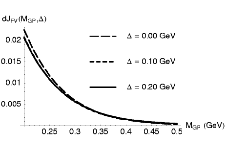
Figure 1: $dJ_{\mathrm{FV}}(M_{\mathrm{GP}},\Delta)$, defined in Eq. (51), plotted against $M_{\mathrm{GP}}$, with three different choices of $\Delta$. This function indicates the deviation (in percent) of the asymptotic form of $J_{\mathrm{FV}}$ from the definition in Eq. (44). The size of the volume in this plot is $L=$2.5 fm. The Goldstone mass $M_{\mathrm{GP}}=0.197$ GeV corresponds to $M_{\mathrm{GP}}L=2.5$, and $M_{\mathrm{GP}}=0.32$ GeV corresponds to $M_{\mathrm{GP}}L=4$. The curve for $\Delta=0.1$ GeV is hidden by that for $\Delta=0.2$ GeV.

The function $J_{\mathrm{FV}}(M_{\mathrm{GP}},\Delta)$ is plotted against $M_{\mathrm{GP}}$ in Fig. 2, with $L=2.5$ fm and three choices of $\Delta$. It is clear from this plot that $\Delta$ can significantly alter the finite volume effects in ${\mathcal{J}}(M_{\mathrm{GP}},\Delta)$.

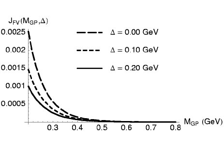
Figure 2: $J_{\mathrm{FV}}(M_{\mathrm{GP}},\Delta)$ plotted as a function of $M_{\mathrm{GP}}$, with three different choices of $\Delta$ corresponding to the three curves. The size of the volume in this plot is $L=$2.5 fm. The Goldstone mass $M_{\mathrm{GP}}=0.197$ GeV corresponds to $M_{\mathrm{GP}}L=2.5$, and $M_{\mathrm{GP}}=0.32$ GeV corresponds to $M_{\mathrm{GP}}L=4$.

Another typical sum that appears in one-loop HM$\chi$PT in finite volume is

$${\mathcal{K}}(M_{\mathrm{GP}},\Delta)=-i\left(\frac{1}{L^{3}}\right)\sum_{\vec{k}}\int\frac{dk_{0}}{2\pi}\left(\frac{1}{k^{2}-M^{2}_{\mathrm{GP}}+i\epsilon}\right)\left(\frac{1}{v\cdot k-\Delta+i\epsilon}\right)^{2}.$$ (52)

It is straightforward to show that

$${\mathcal{K}}(M_{\mathrm{GP}},\Delta)=K(M_{\mathrm{GP}},\Delta)+K_{\mathrm{FV}}(M_{\mathrm{GP}},\Delta),$$ (53)

where

$$K(M_{\mathrm{GP}},\Delta)=\frac{\partial J(M_{\mathrm{GP}},\Delta)}{\partial\Delta}$$ (54)

is the infinite volume limit of ${\mathcal{K}}(M_{\mathrm{GP}},\Delta)$ and

$$K_{\mathrm{FV}}(M_{\mathrm{GP}},\Delta)=\frac{\partial J_{\mathrm{FV}}(M_{\mathrm{GP}},\Delta)}{\partial\Delta}$$ (55)

is the finite volume correction to $K(M_{\mathrm{GP}},\Delta)$. The function $K_{\mathrm{FV}}(M_{\mathrm{GP}},\Delta)$ is plotted against $M_{\mathrm{GP}}$ in Fig. 3, with $L=2.5$ fm and three choices of $\Delta$. As expected, $|K_{\mathrm{FV}}(M_{\mathrm{GP}},\Delta)|$ also decreases when $\Delta$ increases at fixed $M_{\mathrm{GP}}$ and $L$.

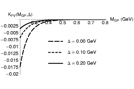
Figure 3: $K_{\mathrm{FV}}(M_{\mathrm{GP}},\Delta)$ plotted as a function of $M_{\mathrm{GP}}$, with three different choices of $\Delta$ corresponding to the three curves. The size of the volume in this plot is $L=2.5$ fm. The Goldstone mass $M_{\mathrm{GP}}=0.197$ GeV corresponds to $M_{\mathrm{GP}}L=2.5$, and $M_{\mathrm{GP}}=0.32$ GeV corresponds to $M_{\mathrm{GP}}L=4$ in this plot.

IV Neutral $B$ mixing and heavy-light decay constants

The study of neutral $B$ meson mixing allows the extraction of the magnitude of the CKM matrix element $V_{td}$, and hence the determination of one of the sides of the unitarity triangle. The frequency of the $B_{d}{-}\bar{B}_{d}$ oscillations, which is given by the mass difference, $\Delta m_{d}$, in this mixing system has been well measured by various experimental collaborations Battaglia:2003in . It is also calculable in the standard model via an operator product expansion in which the top quark and $W$ boson are integrated out. Resumming the next-to-leading order (NLO) short-distance QCD effects, one obtains

$$\Delta m_{d} = \frac{G_{F}}{8\pi^{2}}M^{2}_{W}|V_{td}V^{\ast}_{tb}|^{2}\eta_{B}S_{0}(x_{t})C_{B}(\mu)$$ (56)

$$\times\frac{|\langle\bar{B}_{d}|{\mathcal{O}}^{\Delta B=2}_{d}(\mu)|B_{d}\rangle|}{2M_{B}},$$

where $\mu$ is the renormalisation scale, $x_{t}=m^{2}_{t}/M^{2}_{W}$, and $S_{0}(x_{t})\approx 0.784x_{t}^{0.76}$ (to better than $1\%$) is the relevant Inami-Lim function Inami:1981fz . The coefficients $\eta_{B}=0.55$ and $C_{B}(\mu)$ are from short-distance QCD effects Buras:1990fn ; Buchalla:1996vs . The matrix element of the four-quark operator

$${\mathcal{O}}^{\Delta B=2}_{d}=[\bar{b}\gamma^{\mu}(1-\gamma_{5})d][\bar{b}\gamma_{\mu}(1-\gamma_{5})d]$$ (57)

between $B_{d}$ and $\bar{B}_{d}$ states contains all the long-distance QCD effects in Eq. (56), and has to be calculated non-perturbatively. Since $|V_{tb}|=1$ to good accuracy and $\Delta m_{d}$ has been well measured, a high-precision calculation of $\langle\bar{B}_{d}|{\mathcal{O}}^{\Delta B=2}_{d}(\mu)|B_{d}\rangle$ enables a clean determination of $|V_{td}|$.

The frequency of the rapid $B_{s}{-}\bar{B}_{s}$ oscillations can be precisely measured at the Tevatron and LHC Battaglia:2003in . Therefore an alternative approach is to consider the ratio

$$\frac{\Delta m_{s}}{\Delta m_{d}}=\left|\frac{V_{ts}}{V_{td}}\right|^{2}\left(\frac{M_{B_{d}}}{M_{B_{s}}}\right)\left|\frac{\langle\bar{B}_{s}|{\mathcal{O}}^{\Delta B=2}_{s}|B_{s}\rangle}{\langle\bar{B}_{d}|{\mathcal{O}}^{\Delta B=2}_{d}|B_{d}\rangle}\right|,$$ (58)

in which many theoretical uncertainties cancel. Here $\Delta m_{s}$ is the mass difference in the $B_{s}{-}\bar{B}_{s}$ system and ${\mathcal{O}}^{\Delta B=2}_{s}=[\bar{b}\gamma^{\mu}(1-\gamma_{5})s][\bar{b}\gamma_{\mu}(1-\gamma_{5})s]$. The unitarity of the CKM matrix implies $|V_{ts}|\approx|V_{cb}|$ to a few percent, and $|V_{cb}|$ can be precisely extracted by analysing semileptonic $B$ decays Battaglia:2003in . Therefore a clean measurement of $\Delta m_{s}/\Delta m_{d}$ will yield an accurate determination of $|V_{td}|$.

The matrix elements in Eq. (58) are conventionally parameterised as

$$\langle\bar{B}_{q}|{\mathcal{O}}^{\Delta S=2}_{q}|B_{q}\rangle=\frac{8}{3}M^{2}_{B_{q}}f^{2}_{B_{q}}B_{B_{q}}(\mu),$$ (59)

where the parameter $B_{B_{q}}$ measures the deviation from the vacuum-saturation approximation of the matrix element, and $q=d$ or $s$. The decay constant $f_{B_{q}}$ is defined by

$$\langle 0|\bar{b}\gamma_{\mu}\gamma_{5}q|B_{q}(\vec{p})\rangle=ip_{\mu}f_{B_{q}}.$$ (60)

Lattice QCD provides a reliable tool for calculating these non-perturbative QCD quantities from first principles. Since $\Delta m_{s}/\Delta m_{d}$ will be measured to very good accuracy, it is important to have clean theoretical calculations for [the $SU(3)$ breaking ratios of] the matrix elements, decay constants and $B$ parameters involved. Current lattice calculations have to be combined with effective theories in order to obtain these matrix elements at the physical quark masses. This procedure can introduce significant systematic errors and dominate the uncertainties in the $SU(3)$ breaking ratio Kronfeld:2002ab ; Becirevic:2002mh

$$\xi=\frac{f_{B_{s}}\sqrt{B_{B_{s}}}}{f_{B}\sqrt{B_{B}}},$$ (61)

which is the key theoretical input for future high-precision determination of $|V_{td}|$ via the study of neutral $B$ mixing. However, the use of effective theory also offers a framework for studying finite volume effects in lattice calculations Bernard:1996ez ; Golterman:1997wb ; Sharpe:1992ft ; Golterman:1998st ; Golterman:1998af ; Lin:2002nq ; Lin:2002aj ; Lin:2003tn ; Becirevic:2003wk ; Detmold:2004qn ; Beane:2003da ; Beane:2003yx ; Colangelo:2003hf ; AliKhan:2003cu ; beane:to_appear . We will demonstrate in this section that finite volume effects might turn out to exceed the current quoted systematic errors for quantities such as $\xi$.

IV.1 The one-loop calculation in finite volume

In this subsection, we discuss one-loop calculations for the $B$ parameters and heavy-light decay constants mentioned above in finite volume HM$\chi$PT including the appropriate mass shifts to the first non-trivial order of the chiral and $1/M_{P}$ expansion. The inclusion of other first-order corrections in these quantities is straightforward. It simply introduces additional low-energy constants (LECs) which account for short-distance physics and do not give rise to finite volume effects at this order, so we will not discuss this issue here. We have performed the calculation for full QCD, QQCD and PQQCD with the mass shifts given between Eqs. (25) and (34).

For the purpose of this work, the axial current $\bar{b}\gamma_{\mu}\gamma_{5}q_{a}$ is

$$A_{\mu}=\left(\frac{\kappa}{2}\right){\mathrm{tr}}_{\mathrm{D}}\left[\gamma_{\mu}\gamma_{5}H^{(Q)}_{b}\xi^{\dagger b}_{a}\right],$$ (62)

and the four-quark operator ${\mathcal{O}}^{\Delta P_{a}=2}$ (when $P_{a}=B_{d,s}$, ${\mathcal{O}}^{\Delta P_{a}=2}$ becomes ${\mathcal{O}}^{\Delta B=2}_{d,s}$) is

$$O^{aa} = 4\beta\left[\left(\xi P^{\ast(Q)\dagger}_{\mu}\right)^{a}\left(\xi P^{\ast(\bar{Q})\mu}\right)^{a}\right.$$ (63)

$$\left.+\left(\xi P^{(Q)\dagger}\right)^{a}\left(\xi P^{(\bar{Q})}\right)^{a}\right]$$

in HM$\chi$PT Grinstein:1992qt , where $\kappa$ and $\beta$ are the low-energy constants which have to be determined from experiments or lattice calculations. Notice that the index $a$ in Eq. (63) is not summed over. Again, the inclusion of the chiral and $1/M_{P}$ corrections in these operators simply introduces additional LECs and we do not investigate this aspect here. We assume that $\kappa$ and $\beta$ are the same in full, quenched and partially quenched QCD. Also, $A_{\mu}$ and $O^{aa}$ can couple to the $\eta^{\prime}$ in QQCD, but the couplings are $1/N_{c}$ suppressed Sharpe:1996qp , and we neglect them.

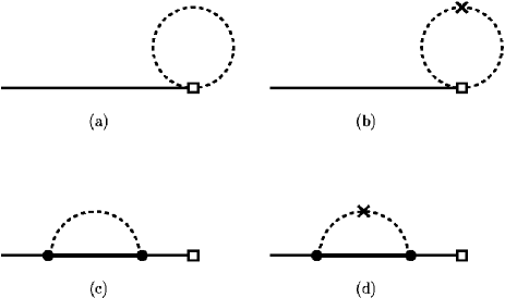
Figure 4: Diagrams contributing to the one-loop calculation of decay constants. The thin (thick) solid lines are the heavy-light pseudoscalar (vector) mesons. The dashed lines are Goldstone particles, and the crosses are the “double poles” which appear in (P)Q$\chi$PT. The open squares are the operators defined in Eq. (62) and the dots are vertices from the HM$\chi$PT Lagrangian. Diagrams (c) and (d) are for wavefunction renormalisation.

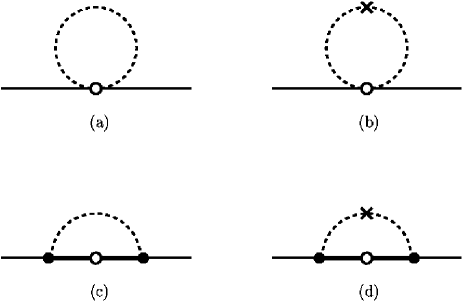
Figure 5: Diagrams contributing to the one-loop calculation of the $B$ parameters. The open circles are the operators defined in Eq. (63).

The diagrams contributing to $f_{P_{(s)}}$ and $B_{P_{(s)}}$ are presented in Figs. 4 and 5 respectively. Only diagrams (c) and (d) depend on the heavy meson mass shifts. Therefore it is the relative weight between these diagrams and the “tadpole” diagrams (a) and (b) which determines the dependence on the heavy meson mass in finite volume effects.

Although this is the first one-loop calculation for these decay constants and $B$ parameters in finite volume, some results in the infinite volume limit already exist in the literature: $f_{P_{(s)}}$ have been calculated at the lowest order in full Grinstein:1992qt , quenched Sharpe:1996qp ; Booth:1995hx and partially quenched Sharpe:1996qp QCD, and up to first-order corrections in the chiral and $1/M_{P}$ expansions in full Boyd:1995pa and quenched QCD Booth:1994rr . The $B$ parameters have been calculated only at lowest order Grinstein:1992qt ; Sharpe:1996qp . Our results, as presented in Appendix B, agree with all these previous calculations in the appropriate limits.

IV.2 Phenomenological impact

We have used the one-loop results in Appendix B to investigate the impact of finite volume effects on $\xi$. In this work, we only intend to estimate the possible size of errors in this quantity, and will leave the actual comparison with lattice data to a future publication. Notice that the one-loop calculation is only valid for $M_{\pi}\ll\Lambda_{\chi}$. Nevertheless, we present our results for $M_{\pi}$ up to $\sim 800\mbox{ MeV}$, where, in principle, higher-order chiral corrections should be included. However, finite volume effects are exponentially suppressed at such large pion masses.

Following the usual procedure in lattice calculations for $\xi$, we study two $SU(3)$ breaking ratios

$$\xi_{f}=\frac{f_{B_{s}}}{f_{B}}$$ (64)

and

$$\xi_{B}=\frac{B_{B_{s}}}{B_{B}},$$ (65)

in terms of which,

$$\xi=\xi_{f}\sqrt{\xi_{B}}.$$ (66)

Furthermore, we define

$$(\xi_{f})_{\mathrm{FV}}\mbox{ }{\mathrm{and}}\mbox{ }(\xi_{B})_{\mathrm{FV}}$$ (67)

to be the contributions from finite volume effects, i.e., those from the volume-dependent part in the one-loop results presented in Subsection IV.1. To be more precise, we use the formulae collected in Appendix B to calculate the volume corrections with respect to the lowest-order values of $f_{B_{s}}$ ($B_{B_{s}}$) and $f_{B}$ ($B_{B}$), then take the difference between the results as an estimate of $(\xi_{f})_{\mathrm{FV}}$ [$(\xi_{B})_{\mathrm{FV}}$]. Since these $SU(3)$ ratios are not very different from unity (at most $\sim 20\%$), this is a reasonable estimate of these effects.

Traditionally, many quenched lattice simulations of $B_{B_{(s)}}$ and $f_{B_{(s)}}$ were performed using $L\sim 1.6$ fm. Therefore we present our estimate for finite volume effects in QQCD with this box size. For comparison, we adopt the same volume for full QCD. As for PQQCD, we work with $L=2.5$ fm where most current high-precision simulations are carried out Davies:2003ik . Throughout this subsection, we ensure that the condition

$$M_{\pi}L\geq 2.5$$ (68)

holds in all the plots presented here.

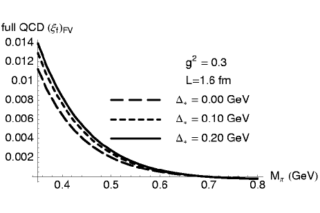
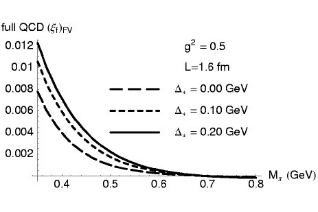
Figure 6: $(\xi_{f})_{\mathrm{FV}}$ in full QCD plotted against $M_{\pi}$, with $L=1.6$ fm. The pion mass $M_{\pi}=0.35$ GeV corresponds to $M_{\pi}L=2.8$, and $M_{\pi}=0.5$ GeV corresponds to $M_{\pi}L=4$ in this plot.

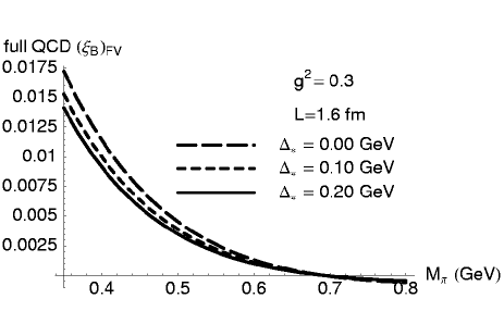
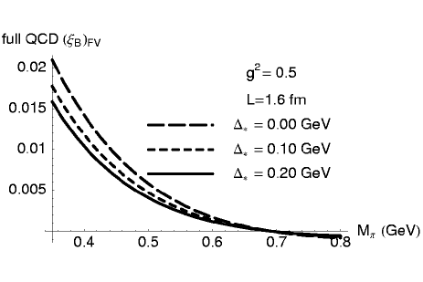
Figure 7: $(\xi_{B})_{\mathrm{FV}}$ in full QCD plotted against $M_{\pi}$, with $L=1.6$ fm. The pion mass $M_{\pi}=0.35$ GeV corresponds to $M_{\pi}L=2.8$, and $M_{\pi}=0.5$ GeV corresponds to $M_{\pi}L=4$ in this plot.

We first discuss the procedure in full and quenched QCD. When studying the light quark mass dependence of $(\xi_{f})_{\mathrm{FV}}$ and $(\xi_{B})_{\mathrm{FV}}$, we follow a strategy similar to that in Ref. Kronfeld:2002ab . That is, we use the Gell-Mann-Okubo formulae to express $M_{K}$ and $M_{\eta}$ in terms of $M_{\pi}$ and $M_{33}$ ($M_{33}$, defined in Eq. (103), is the mass of the fictitious meson composed of $s$ and $\bar{s}$ quarks)

$$M^{2}_{K}=\frac{M^{2}_{33}+M^{2}_{\pi}}{2},$$ (69)

and

$$M^{2}_{\eta}=\frac{2M^{2}_{33}+M^{2}_{\pi}}{3}.$$ (70)

We investigate the situation where a lattice calculation is performed at the physical strange quark mass $(m_{s})_{\mathrm{phys}}$, but the up and down quark mass $m$ is varied. By using $(M_{K})_{\mathrm{phys}}=0.498$ GeV and $(M_{\pi})_{\mathrm{phys}}=0.135$ GeV Hagiwara:2002fs , we fix,

$$(M_{33})_{\mathrm{phys}}=2B_{0}(m_{s})_{\mathrm{phys}}=0.691\mbox{ }{\mathrm{GeV}},$$ (71)

as an input parameter in our analysis. Notice that $(M_{33})_{\mathrm{phys}}$ is not the mass of a “physical” meson, and the subscript just means this mass is estimated by using physical kaon and pion masses. To the same order, we can adopt Eq. (28) to write

$$\delta_{s}=\lambda_{1}\left(M^{2}_{33}-M^{2}_{\pi}\right),$$ (72)

and use $(M_{33})_{\mathrm{phys}}$, $(M_{\pi})_{\mathrm{phys}}$ and physical $M_{B_{s}}-M_{B}=0.091$ GeV Hagiwara:2002fs to determine

$$\lambda_{1}=0.1982\mbox{ GeV}^{-1}.$$ (73)

This determines how $\delta_{s}$ varies with $M_{\pi}$. We have also tried to use vanishing pion mass and $M_{D_{s}}-M_{D}=0.104$ GeV Hagiwara:2002fs to fix $(M_{33})_{\mathrm{phys}}$ and $\lambda_{1}$, and the results presented in this subsection are not sensitive to this variation from the values quoted above.

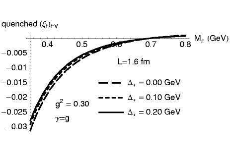
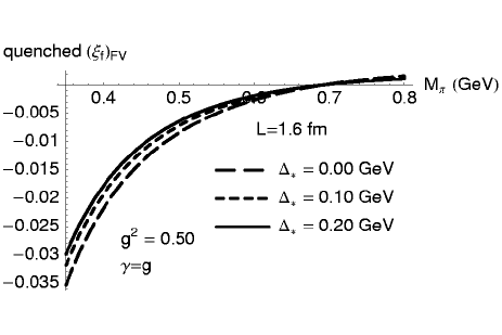
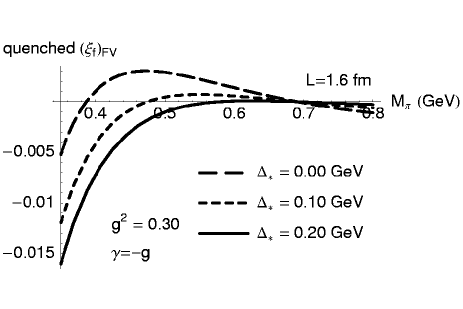
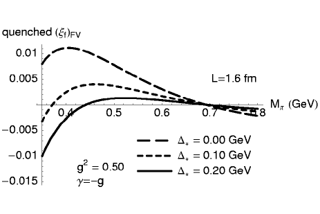
Figure 8: $(\xi_{f})_{\mathrm{FV}}$ in QQCD plotted against $M_{\pi}$, with $L=1.6$ fm and choices of the couplings $g$ and $\gamma$. The pion mass $M_{\pi}=0.35$ GeV corresponds to $M_{\pi}L=2.8$, and $M_{\pi}=0.5$ GeV corresponds to $M_{\pi}L=4$ in this plot. We set $\alpha=0$ and $M_{0}=700$ MeV.

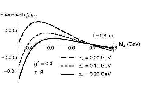
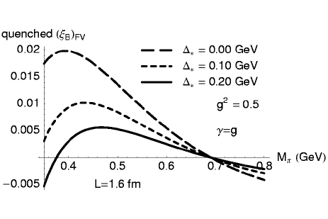
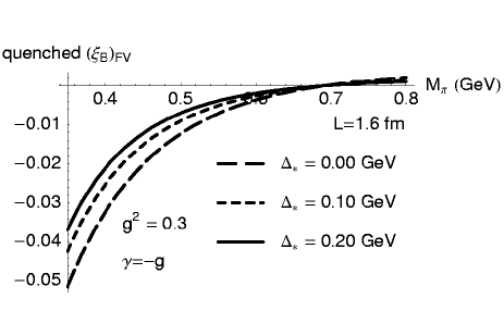
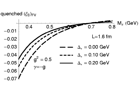
Figure 9: $(\xi_{B})_{\mathrm{FV}}$ in QQCD plotted against $M_{\pi}$, with $L=1.6$ fm and choices of the couplings $g$ and $\gamma$. The pion mass $M_{\pi}=0.35$ GeV corresponds to $M_{\pi}L=2.8$, and $M_{\pi}=0.5$ GeV corresponds to $M_{\pi}L=4$ in this plot. We set $\alpha=0$ and $M_{0}=700$ MeV.

The results for $(\xi_{f})_{\mathrm{FV}}$ and $(\xi_{B})_{\mathrm{FV}}$ for full QCD and QQCD from this analysis are presented in Figs. 6–9, with two different values for the coupling $g$ (and also $\gamma$ in QQCD). Here we stress again that the influence on finite volume effects from the presence of $\Delta_{\ast}$ and $\delta_{s}$ depends on the size of these couplings, which are not well determined. Inspired by the recent CLEO measurement of $g$ in the charm system Ahmed:2001xc ; Anastassov:2001cw , and a recent lattice calculation Abada:2003un , we vary $g^{2}$ between 0.3 and 0.5. As for the coupling $\gamma$, which is a quenching artifact and has never been determined, we vary its value between $g$ and $-g$. It is clear from these plots that the finite volume effects are generally small in full QCD ($\leq 2\%$), but can be significant in QQCD ($\sim 3\%$ to $\sim 7\%$ for $\xi_{B}$) in the range of $M_{\pi}L$ where lattice simulations are normally performed. This is clearly due to the enhanced long-distance effect arising from the “double pole” structure in (P)QQCD, as first pointed out in Ref. Bernard:1996ez , and manifests itself in various places, e.g., nucleon-nucleon potentials Beane:2002vq and $\pi{-}\pi$ scattering Bernard:1996ez ; Golterman:1999hv ; Lin:2003tn ; Lin:2002aj .

Although it has been well established that infinite volume chiral corrections are smaller in the $B$ parameters than in the decay constants due to the coefficient in front of $g^{2}$ in the one-loop results, it is clear from these plots that finite volume effects are more salient in $\xi_{B}$ than in $\xi_{f}$. All the quenched lattice calculations for $\xi_{B}$ have so far concluded that this quantity is consistent with unity with typically $3\%$ error. However, we find that the volume effects are already at the level of $3{-}4\%$ when $M_{\pi}=0.45$ GeV in a 1.6 fm box where many quenched simulations were carried out. This error depends on both light and heavy quark masses in the simulation, hence is amplified after extrapolating the result to the physical quark masses. Also, the fact that volume effects tend towards different directions in full QCD and QQCD when $M_{\pi}$ becomes smaller indicates that quenching errors in these quantities can be larger than those estimated in Ref. Sharpe:1996qp . Since finite volume effects have not been included in the analysis of lattice calculations of $\xi_{B}$ hitherto, one should be cautious when using the existing quenched results for this quantity in any phenomenological work.

For the analysis in PQQCD, we assume that both the valence and sea strange quark masses are fixed at that of the physical strange quark. However, we vary the light sea quark mass $\tilde{m}$. For this purpose, we define $M_{SS}$ to be the mass of the meson composed of two light sea quarks. Therefore,

$$\frac{M^{2}_{SS}}{(M_{33})^{2}_{\mathrm{phys}}}=\left(\frac{\tilde{m}}{\tilde{m}_{s}}\right)_{\tilde{m}_{s}\mbox{ }=\mbox{ }{\mathrm{physical}}\mbox{ }m_{s}}.$$ (74)

Also, we can express the mass shifts $\tilde{\delta}_{s}$ and $\delta_{\mathrm{sea}}$ in terms of meson masses:

$$\tilde{\delta}_{s}=\lambda_{1}\left(M_{33}^{2}-M_{SS}^{2}\right)$$ (75)

and

$$\delta_{\mathrm{sea}}=\lambda_{1}\left(M^{2}_{SS}-M^{2}_{\pi}\right)$$ (76)

by using Eqs. (29) and (30) with the same value of $\lambda_{1}$ as in Eq. (73).

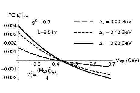
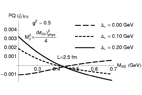
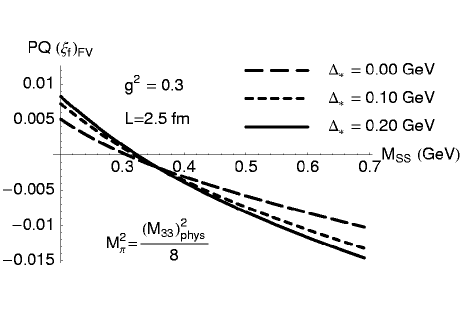
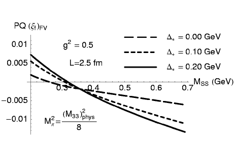
Figure 10: $(\xi_{f})_{\mathrm{FV}}$ in PQQCD plotted against $M_{SS}$ (see text for the definition of $M_{SS}$), with $L=2.5$ fm and two different values for $M_{\pi}$. The pion mass $M^{2}_{\pi}=M^{2}_{33}/4$ corresponds to $M_{\pi}L=4.4$ and $M^{2}_{\pi}=M^{2}_{33}/8$ corresponds to $M_{\pi}L=3.1$. The mass $M_{SS}=0.197$ GeV corresponds to $M_{SS}L=2.5$, and $M_{SS}=0.32$ GeV corresponds to $M_{SS}L=4$ in this plot.

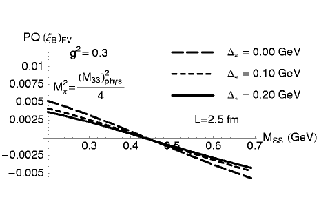
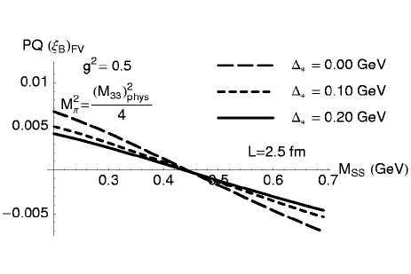
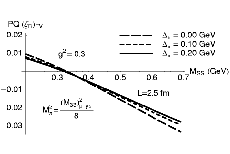
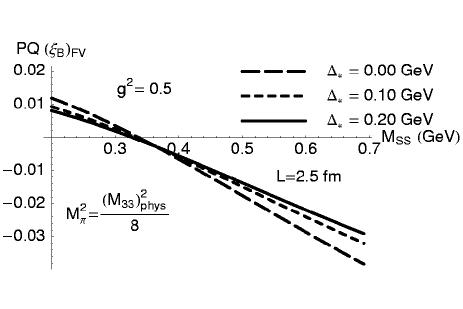
Figure 11: $(\xi_{B})_{\mathrm{FV}}$ in PQQCD plotted against $M_{SS}$ (see text for the definition of $M_{SS}$), with $L=2.5$ fm and two different values for $M_{\pi}$. The pion mass $M^{2}_{\pi}=M^{2}_{33}/4$ corresponds to $M_{\pi}L=4.4$ and $M^{2}_{\pi}=M^{2}_{33}/8$ corresponds to $M_{\pi}L=3.1$. The mass $M_{SS}=0.197$ GeV corresponds to $M_{SS}L=2.5$, and $M_{SS}=0.32$ GeV corresponds to $M_{SS}L=4$ in this plot.

The results for the PQQCD analysis are presented in Figs. 10 and 11. The double pole insertions also appear in PQQCD and it is clear from these plots that finite volume effects cannot be neglected if one hopes to determine $\xi$ to the level of a few percent. Especially, in the range of $M_{\pi}$ and $L$ where current and future lattice simulations are performed Davies:2003ik , they can already be at about $4\%$, and the dependence on the heavy meson mass is quite strong. Therefore they can become comparable to the error presented in the latest review Kronfeld:2003sd ,

$$\xi=1.23\pm 0.10$$ (77)

after quark mass extrapolations.

V Conclusion

We have investigated finite volume effects in heavy quark systems in the framework of heavy meson chiral perturbation theory. The primary conclusion is that the scales $\Delta_{\ast}$ and $\delta_{s}$, which are heavy-light meson mass splittings arising from the breaking of heavy quark spin and light flavour $SU(3)$ symmetries, can significantly reduce the volume effects in diagrams involving heavy meson propagators in the loop. The physical picture of this phenomenon is that some heavy-light mesons are off-shell in the effective theory, as a consequence of the velocity superselection rule, with the virtuality characterised by the mass splittings. The time uncertainty conjugate to this virtuality limits the period during which the Goldstone particles can propagate to the boundary. Finite volume effects caused by the propagation of the Goldstone particles naturally affect the light quark mass extrapolation/interpolation in a lattice calculation. On top of this, our work implies that they also influence the heavy quark mass extrapolation/interpolation, since the scale $\Delta_{\ast}$ varies significantly with the heavy meson mass. The strength of this influence is process-dependent, determined also by the relative weight between diagrams with and without heavy meson propagators in the loop. The volume effects can be amplified by both heavy and light quark mass extrapolations. Therefore it is important to perform calculations to identify these effects in phenomenologically interesting quantities.

We have presented an explicit calculation in finite volume HM$\chi$PT for the $B$ parameters in neutral $B$ meson mixing and heavy-light decay constants, in full, quenched, and partially quenched QCD. We have used these results to estimate the impact of finite volume effects in the $SU(3)$ ratio $\xi$, which is an important input in determining the magnitude of the CKM matrix element $V_{td}$. Within the parameter space where most quenched lattice calculations have been performed, we find that, although this impact is quite small ($\leq\sim 2\%$) in full QCD, it can be significant in QQCD. This is due to the enhanced long-distance effects arising from the double pole structure. This error will be amplified by the quark mass extrapolations and hence can exceed the currently quoted systematic effects. Furthermore, finite volume effects tend towards different directions in full and quenched QCD for decreasing $M_{\pi}$. This means that quenching errors in $\xi$ may be significantly larger than what was estimated before. Therefore one has to be cautious when using the existing quenched lattice QCD results for $\xi$ in phenomenological work. In PQQCD, our results indicate that finite volume effects are typically between $3\%$ and $5\%$ in the data range of future high-precision simulations, and they can be significantly amplified in the procedure of quark mass extrapolations. This means that they are not negligible in future lattice calculations of $\xi$.

Appendix A Integrals and sums

We have regularised ultra-violet divergences that appear in loop integrals using dimensional regularisation, and subtracted the term

$$\bar{\lambda}=\frac{2}{4-d}-\gamma_{E}+{\mathrm{log}}(4\pi)+1.$$ (78)

The integrals appearing in the full QCD calculation are defined by

$$I_{\bar{\lambda}}(m) \equiv \mu^{4-d}\int\frac{d^{d}k}{(2\pi)^{d}}\frac{1}{k^{2}-m^{2}+i\epsilon}$$ (79)

$$= \frac{im^{2}}{16\pi^{2}}\left[\bar{\lambda}-{\log\left(\frac{m^{2}}{\mu^{2}}\right)}\right],$$

$$H_{\bar{\lambda}}(m,\Delta) \equiv \left(g^{\rho\nu}-v^{\rho}v^{\nu}\right)\mu^{4-d}$$ (80)

$$\times\frac{\partial}{\partial\Delta}\int\frac{d^{d}k}{(2\pi)^{d}}\frac{k_{\rho}k_{\nu}}{(k^{2}-m^{2}+i\epsilon)(v\cdot k-\Delta+i\epsilon)}$$

$$= 3\frac{\partial}{\partial\Delta}F_{\bar{\lambda}}(m,\Delta),$$

where

$$F_{\bar{\lambda}}(m,\Delta)=\frac{i}{16\pi^{2}}\bigg{\{}\left[\bar{\lambda}-{\log\left(\frac{m^{2}}{\mu^{2}}\right)}\right]\left(\frac{2\Delta^{2}}{3}-m^{2}\right)\Delta+\left(\frac{10\Delta^{2}}{9}-\frac{4m^{2}}{3}\right)\Delta+\frac{2(\Delta^{2}-m^{2})}{3}mR\left(\frac{\Delta}{m}\right)\bigg{\}},$$ (81)

with

$$R(x)\equiv\sqrt{x^{2}-1}\mbox{ }{\mathrm{log}}\left(\frac{x-\sqrt{x^{2}-1+i\epsilon}}{x+\sqrt{x^{2}-1+i\epsilon}}\right),$$ (82)

and $\mu$ is the renormalisation scale. For the quenched and partially quenched calculations, we also need the integrals

$$I^{(\eta^{\prime})}_{\bar{\lambda}}\equiv\mu^{4-d}\int\frac{d^{d}k}{(2\pi)^{d}}\frac{1}{(k^{2}-m^{2}+i\epsilon)^{2}}=\frac{\partial I_{\bar{\lambda}}(m)}{\partial m^{2}},$$ (83)

and

$$H^{\eta^{\prime}}_{\bar{\lambda}}(m,\Delta) \equiv \left(g^{\rho\nu}-v^{\rho}v^{\nu}\right)\mu^{4-d}$$ (84)

$$\times\frac{\partial}{\partial\Delta}\int\frac{d^{d}k}{(2\pi)^{d}}\frac{k_{\rho}k_{\nu}}{(k^{2}-m^{2}+i\epsilon)^{2}(v\cdot k-\Delta+i\epsilon)}$$

$$= \frac{\partial}{\partial m^{2}}H_{\bar{\lambda}}(m,\Delta).$$

In a cubic spatial box of size $L$ in four dimensions with periodic boundary condition, so that the three-momentum is quantised as in Eq. (41), one obtains the sums (after subtracting the ultra-violet divergences)

$${\mathcal{I}}(m)\equiv\frac{1}{L^{3}}\sum_{\vec{k}}\int\frac{dk_{0}}{2\pi}\frac{1}{k^{2}-m^{2}+i\epsilon}=I(m)+I_{{\mathrm{FV}}}(m),$$ (85)

and

$${\mathcal{H}}(m,\Delta)\equiv\left(g^{\rho\nu}-v^{\rho}v^{\nu}\right)\left(\frac{1}{L^{3}}\right)\sum_{\vec{k}}\frac{\partial}{\partial\Delta}\int\frac{dk_{0}}{2\pi}\frac{k_{\rho}k_{\nu}}{(k^{2}-m^{2}+i\epsilon)(v\cdot k-\Delta+i\epsilon)}=H(m,\Delta)+H_{{\mathrm{FV}}}(m,\Delta)$$ (86)

for the full QCD calculation, where

$$I(m)=I_{\bar{\lambda}}(m)|_{\bar{\lambda}=0},$$ (87)

and

$$H(m)=H_{\bar{\lambda}}(m,\Delta)|_{\bar{\lambda}=0},$$ (88)

are the infinite volume limits of ${\mathcal{I}}$ and ${\mathcal{H}}$, and ($n=|\vec{n}|$)

$$I_{\mathrm{FV}}(m) = \frac{-i}{4\pi^{2}}m\sum_{\vec{n}\not=\vec{0}}\frac{1}{nL}K_{1}\left(nmL\right)$$ (89)

$$\stackrel{{\scriptstyle mL\gg 1}}{{\longrightarrow}} \frac{-i}{4\pi^{2}}\sum_{\vec{n}\not=\vec{0}}\sqrt{\frac{m\pi}{2nL}}\left(\frac{1}{nL}\right){\mathrm{e}}^{-nmL}\times\left\{1+\frac{3}{8nmL}-\frac{15}{128(nmL)^{2}}+{\mathcal{O}}\left(\left[\frac{1}{nmL}\right]^{3}\right)\right\}$$

is the finite volume correction to $I(m)$. The function $H_{\mathrm{FV}}$ is the finite volume correction to $H(m,\Delta)$ and can be obtained via

$$H_{\mathrm{FV}}(m,\Delta)=i\bigg{[}(m^{2}-\Delta^{2})K_{\mathrm{FV}}(m,\Delta)-2\Delta J_{\mathrm{FV}}(m,\Delta)+iI_{\mathrm{FV}}(m)\bigg{]},$$ (90)

where $J_{\mathrm{FV}}(m,\Delta)$ and $K_{\mathrm{FV}}(m,\Delta)$ are defined in Eqs. (44) and (55).

For QQCD and PQQCD calculations, one also needs

$${\mathcal{I}}^{\eta^{\prime}}(m)\equiv\frac{1}{L^{3}}\sum_{\vec{k}}\int\frac{dk_{0}}{2\pi}\frac{1}{(k^{2}-m^{2}+i\epsilon)^{2}}=\frac{\partial I(m)}{\partial m^{2}}+\frac{\partial I_{\mathrm{FV}}(m)}{\partial m^{2}},$$ (91)

and

$${\mathcal{H}}^{\eta^{\prime}}(m,\Delta) \equiv \frac{\partial}{\partial\Delta}\left[\left(g^{\rho\nu}-v^{\rho}v^{\nu}\right)\left(\frac{1}{L^{3}}\right)\sum_{\vec{k}}\int\frac{dk_{0}}{2\pi}\frac{k_{\rho}k_{\nu}}{(k^{2}-m^{2}+i\epsilon)^{2}(v\cdot k-\Delta+i\epsilon)}\right]$$ (92)

$$= \frac{\partial H(m,\Delta)}{\partial m^{2}}+\frac{\partial H_{\mathrm{FV}}(m,\Delta)}{\partial m^{2}}.$$

Appendix B One-loop results for decay constants and $B$ parameters

In this appendix, we collect the results for one-loop corrections to $f_{P_{(s)}}\sqrt{M_{P_{(s)}}}$ and $B_{P_{(s)}}$. For convenience, we introduce

$${\mathcal{C}}_{\pm}(M_{\mathrm{GP}},x)={\mathcal{I}}(M_{\mathrm{GP}})\pm g^{2}{\mathcal{H}}(M_{\mathrm{GP}},x),$$ (93)

and

$${\mathcal{C}}^{\eta^{\prime}}_{\pm}(M_{\mathrm{GP}},x)={\mathcal{I}}^{\eta^{\prime}}(M_{\mathrm{GP}})\pm g^{2}{\mathcal{H}}^{\eta^{\prime}}(M_{\mathrm{GP}},x),$$ (94)

where the functions ${\mathcal{I}}(m)$, ${\mathcal{H}}(m,x)$, ${\mathcal{I}}^{\eta^{\prime}}(m)$ and ${\mathcal{H}}^{\eta^{\prime}}(m,x)$ are defined in Eqs. (85), (86), (91) and (92), respectively.

In full QCD, we find

$$f_{P}\sqrt{M_{P}} = \kappa\bigg{\{}1-\frac{i}{12f^{2}}\bigg{[}9\mbox{ }{\mathcal{C}}_{-}(M_{\pi},\Delta_{\ast})+6\mbox{ }{\mathcal{C}}_{-}(M_{K},\Delta_{\ast}+\delta_{s})+{\mathcal{C}}_{-}(M_{\eta},\Delta_{\ast})\bigg{]}\bigg{\}},$$ (95)

$$f_{P_{s}}\sqrt{M_{P_{s}}} = \kappa\left\{1-\frac{i}{3f^{2}}\bigg{[}3\mbox{ }{\mathcal{C}}_{-}(M_{K},\Delta_{\ast}-\delta_{s})+{\mathcal{C}}_{-}(M_{\eta},\Delta_{\ast})\bigg{]}\right\},$$ (96)

$$B_{P} = \frac{3\beta}{2\kappa^{2}}\left\{1-\frac{i}{6f^{2}}\bigg{[}3\mbox{ }{\mathcal{C}}_{+}(M_{\pi},\Delta_{\ast})+{\mathcal{C}}_{+}(M_{\eta},\Delta_{\ast})\bigg{]}\right\},$$

$$B_{P_{s}} = \frac{3\beta}{2\kappa^{2}}\left\{1-\frac{2i}{3f^{2}}\bigg{[}{\mathcal{C}}_{+}(M_{\eta},\Delta_{\ast})\bigg{]}\right\}.$$ (98)

In QQCD, we find

$$f_{P}\sqrt{M_{P}} = \kappa\bigg{\{}1+\frac{i}{2f^{2}}\bigg{[}\frac{\alpha}{3}{\mathcal{C}}_{-}(M_{\pi},\Delta_{\ast})+\left(\frac{\alpha M^{2}_{\pi}-M^{2}_{0}}{3}\right){\mathcal{C}}^{\eta^{\prime}}_{-}(M_{\pi},\Delta_{\ast})+2g\gamma{\mathcal{H}}(M_{\pi},\Delta_{\ast})\bigg{]}\bigg{\}},$$ (99)

$$f_{P_{s}}\sqrt{M_{P_{s}}} = \kappa\bigg{\{}1+\frac{i}{2f^{2}}\bigg{[}\frac{\alpha}{3}{\mathcal{C}}_{-}(M_{33},\Delta_{\ast})+\left(\frac{\alpha M^{2}_{33}-M^{2}_{0}}{3}\right){\mathcal{C}}^{\eta^{\prime}}_{-}(M_{33},\Delta_{\ast})+2g\gamma{\mathcal{H}}(M_{33},\Delta_{\ast})\bigg{]}\bigg{\}},$$ (100)

$$B_{P} = \frac{3\beta}{2\kappa^{2}}\bigg{\{}1-\frac{i}{f^{2}}\bigg{[}\left(1-\frac{\alpha}{3}\right){\mathcal{C}}_{+}(M_{\pi},\Delta_{\ast})-\left(\frac{\alpha M^{2}_{\pi}-M^{2}_{0}}{3}\right){\mathcal{C}}^{\eta^{\prime}}_{+}(M_{\pi},\Delta_{\ast})+2g\gamma{\mathcal{H}}(M_{\pi},\Delta_{\ast})\bigg{]}\bigg{\}},$$ (101)

$$B_{P_{s}} = \frac{3\beta}{2\kappa^{2}}\bigg{\{}1-\frac{i}{f^{2}}\bigg{[}\left(1-\frac{\alpha}{3}\right){\mathcal{C}}_{+}(M_{33},\Delta_{\ast})-\left(\frac{\alpha M^{2}_{33}-M^{2}_{0}}{3}\right){\mathcal{C}}^{\eta^{\prime}}_{+}(M_{33},\Delta_{\ast})+2g\gamma{\mathcal{H}}(M_{33},\Delta_{\ast})\bigg{]}\bigg{\}},$$ (102)

where

$$M_{33}=\sqrt{2M^{2}_{K}-M_{\pi}^{2}}.$$ (103)

In PQQCD, we find

$$f_{P}\sqrt{M_{P}} = \kappa\bigg{\{}1-\frac{i}{12f^{2}}\bigg{[}12\mbox{ }{\mathcal{C}}_{-}(M_{VS},\Delta_{\ast}+\delta_{\mathrm{sea}})+6\mbox{ }{\mathcal{C}}_{-}(M_{\tau},\Delta_{\ast}+\delta_{\mathrm{sea}}+\tilde{\delta}_{s})$$ (104)

$$\mbox{ }\mbox{ }\mbox{ }\mbox{ }\mbox{ }\mbox{ }\mbox{ }\mbox{ }+3\frac{M^{2}_{33}-M^{2}_{\pi}-2\delta^{2}_{VSs}}{M^{2}_{\pi}-M^{2}_{33}+\delta^{2}_{VS}+2\delta^{2}_{VSs}}{\mathcal{C}}_{-}(M_{\pi},\Delta_{\ast})+\left(\frac{M_{\pi}^{2}-M_{33}^{2}-2\delta^{2}_{VS}+2\delta^{2}_{VSs}}{M_{\pi}^{2}-M_{33}^{2}+\delta^{2}_{VS}+2\delta^{2}_{VSs}}\right)^{2}{\mathcal{C}}_{-}(M_{X},\Delta_{\ast})$$

$$\mbox{ }\mbox{ }\mbox{ }\mbox{ }\mbox{ }\mbox{ }\mbox{ }\mbox{ }\mbox{ }\mbox{ }\mbox{ }\mbox{ }\mbox{ }\mbox{ }\mbox{ }\mbox{ }\mbox{ }\mbox{ }+6\frac{\delta^{2}_{VS}(M_{33}^{2}-M_{\pi}^{2}-2\delta^{2}_{VSs})}{M_{\pi}^{2}-M_{33}^{2}+\delta^{2}_{VS}+2\delta^{2}_{VSs}}{\mathcal{C}}^{\eta^{\prime}}_{-}(M_{\pi},\Delta_{\ast})\bigg{]}\bigg{\}},$$

$$f_{P_{s}}\sqrt{M_{P_{s}}} = \kappa\bigg{\{}1-\frac{i}{6f^{2}}\bigg{[}3\mbox{ }{\mathcal{C}}_{-}(M_{VSs},\Delta_{\ast}+\delta_{\mathrm{sea}}+\tilde{\delta}_{s}-\delta_{s})+6\mbox{ }{\mathcal{C}}_{-}(M_{\zeta s},\Delta_{\ast}+\delta_{\mathrm{sea}}-\delta_{s})$$ (105)

$$\mbox{ }\mbox{ }\mbox{ }\mbox{ }-3\frac{M^{2}_{33}-M^{2}_{\pi}+2\delta^{2}_{VS}}{M^{2}_{33}-M^{2}_{\pi}+2\delta^{2}_{VS}+4\delta^{2}_{VSs}}{\mathcal{C}}_{-}(M_{33},\Delta_{\ast})+2\left(\frac{M_{\pi}^{2}-M_{33}^{2}-2\delta^{2}_{VS}+2\delta^{2}_{VSs}}{M_{\pi}^{2}-M_{33}^{2}-2\delta^{2}_{VS}-4\delta^{2}_{VSs}}\right)^{2}{\mathcal{C}}_{-}(M_{X},\Delta_{\ast})$$

$$\mbox{ }\mbox{ }\mbox{ }\mbox{ }\mbox{ }\mbox{ }\mbox{ }\mbox{ }\mbox{ }\mbox{ }\mbox{ }\mbox{ }\mbox{ }\mbox{ }\mbox{ }\mbox{ }\mbox{ }\mbox{ }\mbox{ }\mbox{ }+6\frac{\delta^{2}_{VSs}(M_{33}^{2}-M_{\pi}^{2}+2\delta^{2}_{VS})}{M_{\pi}^{2}-M_{33}^{2}-2\delta^{2}_{VS}-4\delta^{2}_{VSs}}{\mathcal{C}}^{\eta^{\prime}}_{-}(M_{33},\Delta_{\ast})\bigg{]}\bigg{\}},$$

$$B_{P} = \frac{3\beta}{2\kappa^{2}}\bigg{\{}1-\frac{i}{6f^{2}}\bigg{[}6\mbox{ }{\mathcal{C}}_{+}(M_{\pi},\Delta_{\ast})-3\frac{M^{2}_{\pi}-M^{2}_{33}+2\delta^{2}_{VSs}}{M^{2}_{\pi}-M^{2}_{33}+\delta^{2}_{VS}+2\delta^{2}_{VSs}}{\mathcal{C}}_{+}(M_{\pi},\Delta_{\ast})$$ (106)

$$\mbox{ }\mbox{ }\mbox{ }\mbox{ }\mbox{ }\mbox{ }\mbox{ }\mbox{ }\mbox{ }\mbox{ }\mbox{ }\mbox{ }\mbox{ }\mbox{ }\mbox{ }\mbox{ }\mbox{ }\mbox{ }\mbox{ }\mbox{ }+\left(\frac{M_{\pi}^{2}-M_{33}^{2}-2\delta^{2}_{VS}+2\delta^{2}_{VSs}}{M_{\pi}^{2}-M_{33}^{2}+\delta^{2}_{VS}+2\delta^{2}_{VSs}}\right)^{2}{\mathcal{C}}_{+}(M_{X},\Delta_{\ast})$$

$$\mbox{ }\mbox{ }\mbox{ }\mbox{ }\mbox{ }\mbox{ }\mbox{ }\mbox{ }\mbox{ }\mbox{ }\mbox{ }\mbox{ }\mbox{ }\mbox{ }\mbox{ }\mbox{ }\mbox{ }\mbox{ }\mbox{ }\mbox{ }+6\frac{\delta^{2}_{VS}(M_{33}^{2}-M_{\pi}^{2}-2\delta^{2}_{VSs})}{M_{\pi}^{2}-M_{33}^{2}+\delta^{2}_{VS}+2\delta^{2}_{VSs}}{\mathcal{C}}^{\eta^{\prime}}_{+}(M_{\pi},\Delta_{\ast})\bigg{]}\bigg{\}},$$

$$B_{P_{s}} = \frac{3\beta}{2\kappa^{2}}\bigg{\{}1-\frac{i}{3f^{2}}\bigg{[}3{\mathcal{C}}_{+}(M_{33},\Delta_{\ast})-3\frac{M^{2}_{\pi}-M^{2}_{33}-2\delta^{2}_{VS}}{M^{2}_{\pi}-M^{2}_{33}-2\delta^{2}_{VS}-4\delta^{2}_{VSs}}{\mathcal{C}}_{+}(M_{33},\Delta_{\ast})$$ (107)

$$\mbox{ }\mbox{ }\mbox{ }\mbox{ }\mbox{ }\mbox{ }\mbox{ }\mbox{ }\mbox{ }\mbox{ }\mbox{ }\mbox{ }\mbox{ }\mbox{ }\mbox{ }\mbox{ }\mbox{ }\mbox{ }\mbox{ }\mbox{ }+2\left(\frac{M_{\pi}^{2}-M_{33}^{2}-2\delta^{2}_{VS}+2\delta^{2}_{VSs}}{M_{\pi}^{2}-M_{33}^{2}-2\delta^{2}_{VS}-4\delta^{2}_{VSs}}\right)^{2}{\mathcal{C}}_{+}(M_{X},\Delta_{\ast})$$

$$\mbox{ }\mbox{ }\mbox{ }\mbox{ }\mbox{ }\mbox{ }\mbox{ }\mbox{ }\mbox{ }\mbox{ }\mbox{ }\mbox{ }\mbox{ }\mbox{ }\mbox{ }\mbox{ }\mbox{ }\mbox{ }\mbox{ }\mbox{ }+6\frac{\delta^{2}_{VSs}(M_{33}^{2}-M_{\pi}^{2}+2\delta^{2}_{VS})}{M_{\pi}^{2}-M_{33}^{2}-2\delta^{2}_{VS}-4\delta^{2}_{VSs}}{\mathcal{C}}^{\eta^{\prime}}_{+}(M_{33},\Delta_{\ast})\bigg{]}\bigg{\}},$$

where

$$M_{VS}^{2}=B_{0}(m+\tilde{m}) \mbox{ }\mbox{ }M_{VSs}^{2}=B_{0}(m_{s}+\tilde{m}_{s}),$$ ,

$$M_{\tau}^{2}=B_{0}(m+\tilde{m}_{s})=M^{2}_{VSs}-M^{2}_{K}+M^{2}_{\pi} \mbox{ }\mbox{ }M_{\zeta s}^{2}=B_{0}(m_{s}+\tilde{m})=M^{2}_{VS}+M^{2}_{K}-M^{2}_{\pi},$$ ,

$$\delta^{2}_{VS}=M^{2}_{\pi}-M^{2}_{VS} \mbox{ }\mbox{ }\delta^{2}_{VSs}=M^{2}_{33}-M^{2}_{VSs},$$ ,

$${\mathrm{and}}\mbox{ }\mbox{ }M_{X}^{2} = \frac{1}{3}\left(M^{2}_{\pi}+2M^{2}_{33}-2\delta^{2}_{VS}-4\delta^{2}_{VSs}\right).$$ (108)

It is straightforward to show that the PQQCD results reproduce those for full QCD in the limit $\tilde{m}=m$ and $\tilde{m}_{s}=m_{s}$.

References

- (1) M. Battaglia et al., hep-ph/0304132, to appear as CERN Yellow Report.
- (2) J. Gasser and H. Leutwyler, Phys. Lett. B188, 477 (1987).
- (3) H. Leutwyler and A. Smilga, Phys. Rev. D46, 5607 (1992).
- (4) K. Hagiwara et al., Phys. Rev. D66, 010001 (2002).
- (5) S. Beane, hep-lat/0403015.
- (6) C. W. Bernard and M. F. L. Golterman, Phys. Rev. D53, 476 (1996).
- (7) C. W. Bernard and M. F. L. Golterman, Phys. Rev. D46, 853 (1992).
- (8) C. W. Bernard and M. F. L. Golterman, Phys. Rev. D49, 486 (1994).
- (9) S. R. Sharpe and N. Shoresh, Phys. Rev. D64, 114510 (2001).
- (10) S. R. Sharpe and N. Shoresh, Phys. Rev. D62, 094503 (2000).
- (11) G. Burdman and J. F. Donoghue, Phys. Lett. B280, 287 (1992).
- (12) M. B. Wise, Phys. Rev. D45, 2188 (1992).
- (13) T.-M. Yan et al., Phys. Rev. D46, 1148 (1992).
- (14) M. J. Booth, Phys. Rev. D51, 2338 (1995).
- (15) S. R. Sharpe and Y. Zhang, Phys. Rev. D53, 5125 (1996).
- (16) C. G. Boyd and B. Grinstein, Nucl. Phys. B442, 205 (1995).
- (17) M. J. Booth, hep-ph/9412228.
- (18) B. Grinstein et al., Nucl. Phys. B380, 369 (1992).
- (19) H. Georgi, Phys. Lett. B240, 447 (1990).
- (20) T. Inami and C. S. Lim, Prog. Theor. Phys. 65, 297 (1981).
- (21) A. J. Buras, M. Jamin, and P. H. Weisz, Nucl. Phys. B347, 491 (1990).
- (22) G. Buchalla, A. J. Buras, and M. E. Lautenbacher, Rev. Mod. Phys. 68, 1125 (1996).
- (23) J. M. Flynn and C. T. Sachrajda, Adv. Ser. Direct. High Energy Phys. 15, 402 (1998).
- (24) C. T. Sachrajda, Nucl. Instrum. Meth. A462, 23 (2001).
- (25) J. Flynn and C.-J. D. Lin, J. Phys. G27, 1245 (2001).
- (26) C. W. Bernard, Nucl. Phys. Proc. Suppl. 94, 159 (2001).
- (27) S. M. Ryan, Nucl. Phys. Proc. Suppl. 106, 86 (2002).
- (28) N. Yamada, Nucl. Phys. Proc. Suppl. 119, 93 (2003).
- (29) L. Lellouch, Nucl. Phys. Proc. Suppl. 117, 127 (2003).
- (30) D. Becirevic, hep-ph/0310072.
- (31) A. S. Kronfeld, hep-lat/0310063.
- (32) A. S. Kronfeld and S. M. Ryan, Phys. Lett. B543, 59 (2002).
- (33) D. Becirevic, S. Fajfer, S. Prelovsek, and J. Zupan, Phys. Lett. B563, 150 (2003).
- (34) M. F. L. Golterman and K. C. Leung, Phys. Rev. D56, 2950 (1997).
- (35) M. F. L. Golterman and K.-C. Leung, Phys. Rev. D57, 5703 (1998).
- (36) M. F. L. Golterman and K.-C. Leung, Phys. Rev. D58, 097503 (1998).
- (37) C.-J. D. Lin et al., Nucl. Phys. B650, 301 (2003).
- (38) C.-J. D. Lin et al., Phys. Lett. B553, 229 (2003).
- (39) C.-J. D. Lin et al., Phys. Lett. B581, 207 (2004).
- (40) D. Becirevic and G. Villadoro, hep-lat/0311028.
- (41) W. Detmold and M. J. Savage, hep-lat/0403005.
- (42) S. R. Beane, P. F. Bedaque, A. Parreno, and M. J. Savage, hep-lat/0312004.
- (43) S. R. Beane, P. F. Bedaque, A. Parreno, and M. J. Savage, nucl-th/0311027.
- (44) G. Colangelo and S. Durr, hep-lat/0311023.
- (45) A. Ali Khan et al., hep-lat/0312030.
- (46) S. R. Sharpe, Phys. Rev. D46, 3146 (1992).
- (47) C. T. H. Davies et al., Phys. Rev. Lett. 92, 022001 (2004).
- (48) S. Ahmed et al., Phys. Rev. Lett. 87, 251801 (2001).
- (49) A. Anastassov et al., Phys. Rev. D65, 032003 (2002).
- (50) A. Abada et al., JHEP 02, 016 (2004).
- (51) S. R. Beane and M. J. Savage, Nucl. Phys. A709, 319 (2002).
- (52) M. Golterman and E. Pallante, Nucl. Phys. Proc. Suppl. 83, 250 (2000).