Abstract

We investigate a new numerical procedure to compute fermionic correlation functions at very small quark masses. Large statistical fluctuations, due to the presence of local “bumps” in the wave functions associated with the low-lying eigenmodes of the Dirac operator, are reduced by an exact low-mode averaging. To demonstrate the feasibility of the technique, we compute the two-point correlator of the left-handed vector current with Neuberger fermions in the quenched approximation, for lattices with a linear extent of $L\approx 1.5$ fm, a lattice spacing $a\approx 0.09$ fm, and quark masses down to the $\epsilon$-regime. By matching the results with the corresponding (quenched) chiral perturbation theory expressions, an estimate of (quenched) low-energy constants can be obtained. We find agreement between the quenched values of $F$ extrapolated from the $p$-regime and extracted in the $\epsilon$-regime.

March 2004

1 Introduction

One of the most important challenges for lattice QCD is the simulation of quarks with masses light enough to reach kinematical regions where chiral perturbation theory (ChPT) [1, 2] can be verified and safely applied. Despite valuable efforts in the infinite-volume limit [3]-[6], it is still unclear how small the quark masses need to be in order to reach the chiral region (for recent developments, see [7, 8]). More recently the $\epsilon$-regime of QCD [9, 10], in which $m\rightarrow 0$ at finite volume $V$, is being attacked on the lattice [11, 12, 13, 5, 14, 15, 16]. Difficulties to reach these kinematical corners arise because most of the numerical techniques currently used on the lattice become inefficient when the quark masses approach the chiral limit.
In the presence of spontaneous chiral symmetry breaking, chiral perturbation theory suggests that the low-lying eigenvalues of the massless QCD Dirac operator scale proportionally to $(\Sigma V)^{-1}$, where $\Sigma$ is the bare quark condensate and $V$ is the lattice volume [9, 17]. In addition random matrix theory [18, 19] (and to some extent quenched ChPT [20]) predicts the distribution of each individual eigenvalue as a function of $\Sigma V$. Comparisons of these predictions with numerical data obtained on the lattice in quenched QCD have been reported by several collaborations [21, 11, 14, 15]. Only recently has an extensive study of this issue, performed at several volumes and lattice spacings, shown a detailed agreement between some of these predictions and quenched QCD for volumes larger than about $5$ fm⁴ [15]. No predictions are available for the properties of the corresponding wave functions (for a recent compilation of numerical results, see [22]). It is an empirical observation, though, that they can develop local “bumps” with a non-negligible probability [15].
It is then conceivable to exploit such basic properties of QCD as suggested by ChPT to develop exact and generic numerical algorithms which remain efficient when the quark masses approach the chiral regime. For instance, due to the scaling of the low-lying eigenvalues with $V$, the computation of the fermion propagator with standard techniques becomes very demanding when the quark masses approach the chiral limit, since the Dirac operator tends to be strongly ill-conditioned. The slow-down can be dramatically reduced by subtracting a few of the lowest modes and treating them separately [23].
In this paper we propose a new technique to compute QCD fermionic correlation functions at very small quark masses on the lattice. An exact low-mode averaging procedure is introduced to reduce large statistical fluctuations induced by the presence of “bumps” in the wave functions associated with the low-lying eigenvalues of the Dirac operator which happen to occur where the fermionic operators are localized. The feasibility of the technique is proven by computing the correlator of two left-handed vector currents in quenched QCD with Neuberger fermions [24]-[30]. We find that the variance of the estimate is markedly reduced with respect to the one with standard techniques when the quark mass is decreased, and the $\epsilon$-regime can be safely reached in all topological sectors.
The use of the quenched approximation mainly serves to test our method, which we expect will be effective for simulations of full QCD as well. It is known that the quenched theory is afflicted with several problems. In particular, the removal of the fermion determinant renders the theory non-unitary. An effective low-energy description of the quenched theory is formally obtained if an additional expansion in $1/N_{c}$, where $N_{c}$ is the number of colors, is carried out together with the usual one in quark masses and momenta. The resulting so-called quenched ChPT [32, 33] leads to infrared divergences in certain correlation functions. These divergences reflect, at least partially, the sickness of quenched QCD. Here we adopt the pragmatic assumption that – despite the fact that it is not an asymptotic expansion of quenched QCD (at fixed $N_{c}$) – quenched ChPT describes the low-energy regime of quenched QCD in certain ranges of kinematical scales, where correlation functions can be parameterized in terms of effective coupling constants, the latter being defined as the couplings which appear in the Lagrangian of the effective theory. With this assumption in mind we compare the predictions of quenched ChPT with the numerical results obtained in the kinematically accessible ranges in the $p$- and $\epsilon$-regimes for the correlator of two left-handed currents. Thereby we estimate values of $F$ and $\alpha_{5}$ (to be defined below), which, according to our working assumption, are then identified with quenched versions of the physical LECs.
It is interesting to note that the correlator of two left-handed vector currents is free from zero-mode contributions and, at fixed volume, remains finite when the quark mass $m\rightarrow 0$. This is in contrast to the correlators of two scalar or pseudoscalar densities in sectors of non-zero topological charge at finite volume. They develop $1/m^{2}$ divergences with residues given by correlation functions of zero-mode wave functions [16]. Since in both cases the leading non-trivial behaviour is governed by $F$, these two different types of correlators offer independent determinations of this coupling.
The paper is organized as follows: in Sect. 2 we collect the formulæ for the two-point correlation function of the left-handed vector current in chiral perturbation theory, in Sect. 3 we describe the low-mode averaging procedure for fermionic correlation functions, and in Sect. 4 we report the details of the simulations we have performed in quenched QCD, as well as the results obtained. We conclude in Sect. 5. In the first Appendix we provide more details of our notations, and in the second we collect further useful formulæ obtained in ChPT at finite volume.

2 Left-handed current correlator in ChPT

We start by considering the physical, unquenched QCD. The Euclidean Lagrangian of the chiral effective theory for this case reads, at leading order in the momentum expansion,

$${\cal L}=\frac{F^{2}}{4}\,\mbox{Tr}\;\left\{\partial_{\mu}U^{\dagger}\partial_{\mu}U\right\}-\frac{\Sigma}{2}\,\mbox{Tr}\;\left\{e^{i\theta/N_{\rm f}}UM+M^{\dagger}U^{\dagger}e^{-i\theta/N_{\rm f}}\right\}\,,$$ (1)

where $U\in$ SU($N_{\rm f}$) is the meson field, $N_{\rm f}=3$, $M=\mathop{\mbox{diag}}(m_{u},m_{d},m_{s})$ the quark mass matrix, $\theta$ the vacuum angle, and, in the chiral limit, $F$ equals the pseudoscalar decay constant and $\Sigma$ the chiral condensate . At the next-to-leading order (NLO) in the momentum expansion, additional operators appear in the effective Lagrangian, with the associated LECs $\alpha_{1},\alpha_{2},...$ [2] . In the following we consider only the case of a degenerate mass matrix, i.e. $m_{u}=m_{d}=m_{s}\equiv m$.
The LECs can be determined by computing suitable QCD correlation functions on the lattice at small masses and momenta, and by comparing the results with the parameterization given by ChPT. In this paper we are interested in the two-point correlation function [23, 34]

$${\cal C}^{ab}(t)=\int{\rm d}^{3}x\,\langle{\cal J}^{a}_{0}(x){\cal J}^{b}_{0}(0)\rangle$$ (2)

of the left-handed charge density ${\cal J}^{a}_{0}(x)$, where $t=x_{0}$. In the effective theory, at the leading order in momentum expansion, it reads

$${\cal J}^{a}_{0}=\frac{F^{2}}{2}\,\mbox{Tr}\;\left\{\mbox{T}^{a}U\partial_{0}U^{\dagger}\right\}$$ (3)

where $\mbox{T}^{a}$ is a traceless generator of SU($N_{\rm f}$), acting on flavor indices, and on the side of QCD we assumed the normalization of Eq. (20) below.
A kinematical range of scales which is suitable for extracting the LECs in a finite box of volume $V=TL^{3}$, is the so-called $p$-regime. It is defined by the constraints $M_{P}L\mathop{\raise 1.29167pt\hbox{$>$\kern-7.5pt\raise-4.73611pt\hbox{$\sim$}}}1$ and $M_{P}\ll 4\pi F$, where $M_{P}$ is the pseudoscalar meson mass. Writing $\mathcal{C}^{ab}(t)\equiv\mbox{Tr}\;[\mbox{T}^{a}\mbox{T}^{b}]\,\mathcal{C}(t)$, the next-to-leading order (NLO) finite-volume prediction can be expressed as [36]

$$\mathcal{C}(t)=\frac{1}{2}M_{P}^{V}(F_{P}^{V})^{2}\frac{\cosh\Bigl{[}(T/2-|t|)M_{P}^{V}\Bigr{]}}{2\sinh\Bigl{[}TM_{P}^{V}/2\Bigr{]}}-\frac{N_{\rm f}}{2}\frac{{\rm d}g_{1}}{{\rm d}T}\,,$$ (4)

where

$$F_{P}^{V} \equiv F_{P}\biggl{(}1-\frac{N_{\rm f}g_{1}}{2F_{P}^{2}}\biggr{)}\;,$$ (5)

$$F_{P} = F\biggl{[}1-\frac{N_{\rm f}G(M^{2})}{2F^{2}}+\frac{M^{2}}{2(4\pi F)^{2}}\Bigl{(}N_{\rm f}\alpha_{4}+\alpha_{5}\Bigr{)}\biggr{]}\;,$$ (6)

and $M^{2}=2m\Sigma/F^{2}$. The effective finite-volume meson mass $M_{P}^{V}$ and the functions $g_{1}$ and $G(M^{2})$ are reported in Appendix B. Finite-volume effects are exponentially small if $M_{P}L\gg 1$, and we can set $g_{1}=0$.
A less explored kinematical region of QCD, where the LECs can be extracted, is the so-called $\epsilon$-regime, where $M_{P}L\ll 1$ and the linear extent of the box is such that $4\pi FL\gg 1$ [9, 10]. In this regime topology plays an important rôle [17], and for fixed topological charge $\nu$ [36, 37, 34]

$$\mathcal{C}(t)=\frac{F^{2}}{2T}\biggl{[}1+\frac{N_{\rm f}}{F^{2}}\biggl{(}\frac{\beta_{1}}{\sqrt{V}}-\frac{T^{2}k_{00}}{V}\biggr{)}+\frac{2\mu T^{2}}{F^{2}V}\sigma_{\nu}(\mu)h_{1}\Bigl{(}\frac{t}{T}\Bigr{)}\biggr{]}\;,$$ (7)

where $\mu\equiv m\Sigma V$ and

$$h_{1}\left(\frac{t}{T}\right)=\frac{1}{2}\left[\Big{(}\Big{|}\frac{t}{T}\Big{|}-\frac{1}{2}\Big{)}^{2}-\frac{1}{12}\right]\,.$$ (8)

The constants $\beta_{1}$ and $k_{00}$ are related to the (dimensionally regularized) value of

$$\bar{G}(0)=\frac{1}{V}\sum_{n\in\mbox{\raisebox{-0.60275pt}{$\scriptstyle\mathsf{ZZ}^{4}$}}}\Bigl{(}1-\delta^{(4)}_{n,0}\Bigr{)}\frac{1}{p^{2}}\;,\quad p=2\pi\Bigl{(}\frac{n_{0}}{T},\frac{\vec{n}}{L}\Bigr{)}\;,$$ (9)

by

$$\bar{G}(0)\equiv-\frac{\beta_{1}}{\sqrt{V}}\;,\quad T\frac{{\rm d}}{{\rm d}T}\bar{G}(0)\equiv\frac{T^{2}k_{00}}{V}\;.$$ (10)

Furthermore $\sigma_{\nu}(\mu)\equiv{N_{\rm f}}^{-1}{\rm d}\{\ln\det[I_{\nu+j-i}(\mu)]\}/{\rm d}\mu$, where the determinant is taken over an $N_{\rm f}\times N_{\rm f}$ matrix, whose matrix element $(i,j)$ is the modified Bessel function $I_{\nu+j-i}$ [38, 17].
In ChPT there is a well-defined prescription to compute correlation functions at fixed topology, and here we assume that also in QCD they have a well-defined meaning in the continuum limit at non-zero physical distances. Although plausible, this is a non-trivial dynamical issue and to pose precise questions we must introduce an ultraviolet regularization. We here adopt a lattice regularization with fermions discretized à la Neuberger [28]. The massless Dirac operator obeys the Ginsparg-Wilson (GW) relation and therefore preserves an exact chiral symmetry. The topological index assigned to a configuration is $\nu=n_{+}-n_{-}$, where $n_{+}$ ($n_{-}$) are the numbers of zero-modes of $D$ with positive (negative) chirality. Our working hypothesis is that correlators of composite operators at non-zero physical distance have a continuum limit in any given sector of index $\nu$ independent of the particular choice of $D$ . Some recent numerical evidence (in the quenched approximation) consistent with this scenario can be found, e.g. in Refs. [15, 39].
In quenched ChPT the flavor singlet field cannot be integrated out and therefore additional coupling constants appear in the chiral Lagrangian [32, 33]. In particular the singlet mass parameter $m^{2}_{0}/2N_{c}$ is dimensionful and, even if suppressed by large-$N_{c}$ counting, cannot be tuned by changing the kinematical conditions. Consequently, the standard chiral expansion is expected to be useful only in a window of Euclidean momenta $q^{2}$, where $m_{0}^{2}/2N_{c}\ll q^{2}\ll(4\pi F)^{2}$.
In the quenched theory, Eq. (4) remains the same, apart from the omission of the last constant term $\propto N_{\rm f}$, but at NLO the interpretation of the parameters in terms of those of quenched ChPT changes [40] . In particular, the parameter $F_{P}^{V}$ is volume-independent,

$$F_{P}^{V}=F_{P}=F\biggl{[}1+\frac{M^{2}}{2(4\pi F)^{2}}\alpha_{5}\biggr{]}\,,\\$$ (11)

where the LEC $\alpha_{5}$ is finite at this order. In the $\epsilon$-regime, on the other hand, the correlator of two left-handed vector charges is modified to be [37, 34]

$${\cal C}(t)=\frac{F^{2}}{2T}\left\{1+\frac{2\mu T^{2}}{F^{2}V}\sigma_{\nu}(\mu)h_{1}\Big{(}\frac{t}{T}\Big{)}\right\}\,,$$ (12)

where in this case [41]

$$\sigma_{\nu}(\mu)=\mu\Big{\{}I_{\nu}(\mu)K_{\nu}(\mu)+I_{\nu+1}(\mu)K_{\nu-1}(\mu)\Big{\}}+\frac{\nu}{\mu}\,,$$ (13)

and $I_{\nu}$ and $K_{\nu}$ are modified Bessel functions.

3 Low-mode averaging

Although the technique we are going to describe can be more widely applied, we restrict ourselves to lattices of spacing $a$, volume $V=TL^{3}$ and with periodic boundary conditions imposed on all fields. QCD gluons and fermions are discretized using the standard plaquette Wilson action and the Neuberger-Dirac operator $D$, respectively. The latter [28] satisfies the Ginsparg-Wilson relation [24]

$$\gamma_{5}D+D\gamma_{5}=\bar{a}D\gamma_{5}D\,,$$ (14)

and thus preserves an exact chiral symmetry at finite lattice spacing [29]. The Neuberger operator, the parameter $\bar{a}$ and other conventions used in this section are defined in Appendix A, and are the same as in Ref. [23]. The massive lattice Dirac operator is given by

$$D_{m}=(1-\frac{\bar{a}m}{2})D+m$$ (15)

where $0\leq\bar{a}m\leq 2$. For a given gauge configuration the massless Dirac operator can be diagonalized, and chirality implies that non-chiral modes appear in complex conjugate pairs, i.e.

$$D\eta_{\lambda_{k}} = \lambda_{k}\,\eta_{\lambda_{k}}\,,\qquad k=1,2,\dots\,,$$ (16)

$$D\eta_{\lambda^{*}_{k}} = \lambda^{*}_{k}\eta_{\lambda^{*}_{k}}\,,\qquad\eta_{\lambda^{*}_{k}}=\gamma_{5}\eta_{\lambda_{k}}\,.$$ (17)

Random matrix theory [18, 19] (and to some extent quenched ChPT [20]) predicts the probability distribution of each eigenvalue in the low-lying end of the spectrum to be a function of the rescaled variable $\zeta=|\lambda|\Sigma V$ only. Some of these predictions are reported in Fig. 1 for the quenched theory. In particular, the predicted individual distributions of the first four eigenvalues together with the total microscopic density for $\nu=0$ are shown in the plot on the left, while the individual distributions of the first non-zero eigenvalue are shown for several values of $\nu$ in the right plot. It is interesting to note that there is no gap for small values of $\zeta$, and the total distribution is predicted to be $\rho_{s}(\zeta)\sim\zeta^{2(|\nu|+N_{\rm f})+1}$. Therefore arbitrarily small eigenvalues can occur (either in the full or the quenched theory) with a probability which decreases exponentially with $|\nu|$ and $N_{\rm f}$. The expectation value of the lowest eigenvalue and the level splittings near the origin are of $O(1/\Sigma V)$, as can be seen in Fig. 1. The ratios of expectation values of low-lying eigenvalues are then parameter-free predictions of RMT, and they have been confronted with quenched QCD data in Ref. [15]. An impressive agreement has been found for volumes larger than about $5$ fm⁴.

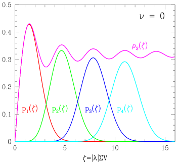
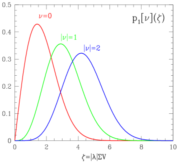
Figure 1: Probability density distributions of low-lying eigenvalues in quenched QCD. Left: distributions of the first four eigenvalues ${\rm p}_{i}(\zeta)$ $(i=1,\dots 4)$ and of the microscopic total density $\rho_{s}(\zeta)$ for $\nu=0$. Right: distributions of the first eigenvalue for $|\nu|=0,1,2$.

No analytic predictions are available so far for the properties of the corresponding wave functions. In Ref. [15] it was found that the probability distribution of their norm at a fixed lattice site is broader than the one expected for a normalized random vector. Since in the following we are interested in the correlation function of two left-handed currents, we have studied the probability distribution of $u=|{\rm Re}[v_{11}(x)]|V$, where

$$v_{kl}(x)=[\eta_{\lambda_{k}}^{\dagger}\gamma_{0}P_{-}\eta_{\lambda_{l}}](x)\,,$$ (18)

on a lattice of volume $16^{4}$ at $\beta=6.0$ (Lattice B, see next section). The result is shown in Fig. 2 together with the analogous prediction for the case that the $\eta$’s are treated as random vectors with unit norm and such that $\sum_{x}[\eta_{\lambda_{k}}^{\dagger}\gamma_{5}\eta_{\lambda_{k}}](x)=0$. As can be seen from the inset in the figure, the distribution decreases quite slowly, and thus the probability of finding a point on the lattice for which $u$ exceeds its mean value by far is quite high: for instance, the probability for finding $u\geq 0.5$ is $0.7\%$. We also mention that the distribution of $|{\rm Im}[v_{11}(x)]|V$ nicely overlaps with the one reported in Fig. 2.

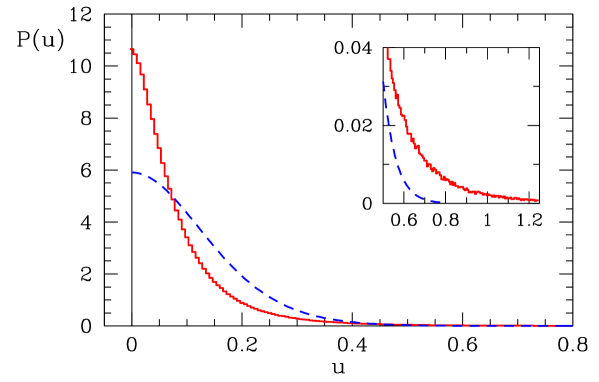
Figure 2: Probability distribution of $u=|{\rm Re}[v_{11}(x)]|V$ (cf. Eq.(18)) for the first normalized non-zero mode eigenvector of $D$. The solid line is the distribution obtained at $\beta=6.0$ on a $16^{4}$ lattice (Lattice B, see below), while the dashed curve is the one expected for a random vector model.

These properties of eigenvalues and eigenfunctions of the Dirac operator imply that, when a fermionic correlation function is computed with standard Monte Carlo techniques, the relative contributions from the various eigenvalues can change dramatically with $m$:

• for $m\gg 1/\Sigma V$, the low-lying end of the spectrum of $D_{m}$ is very dense near $m$, and (many) contributions from the corresponding wave-functions are averaged with essentially the same weight.

• for $m\sim 1/\Sigma V$, the mass is comparable with the expectation value of the modulus of the lowest eigenvalue of $D$ (see Fig. 1), and therefore the low-lying spectrum of $D_{m}$ appears discrete (the splittings of the eigenvalues are of the same order as their values). The contribution of just a few eigenvectors to a given observable can be substantial and their space-time fluctuations can then induce large fluctuations in its estimate. A significant improvement can be achieved in this case by low-mode averaging as we explain in the remainder of this section.

• for $m\ll 1/\Sigma V$, the mass is much smaller than the expectation value of the lowest eigenvalue of $D$. Extremely small eigenvalues of $D_{m}$ can then occur with a small but non-negligible probability. The standard Monte Carlo sampling of the path integral for fermionic correlation functions is problematic in this case, because a sizeable contribution to the estimate of these integrals is obtained from configurations that have a small statistical weight (i.e., those with the smallest eigenvalues of $D_{m}$, for which these observables are very large). We did not find a straightforward solution to this problem. It would probably require an improved algorithm where the low-mode contribution to the observable is included in the Monte Carlo sampling of the integral. If such an algorithm exists, it will presumably be very expensive in practice.

The information above can be exploited in order to develop efficient algorithms for computing fermionic correlation functions in the regime $m\mathop{\raise 1.29167pt\hbox{$>$\kern-7.5pt\raise-4.73611pt\hbox{$\sim$}}}1/\Sigma V$. In the following we focus on the two-point function

$$C^{ab}(t)=\sum_{\bf\vec{x}}\langle J^{a}_{0}(x)J^{b}_{0}(0)\rangle$$ (19)

of two left-handed charge densities,

$$J^{a}_{0}(x)=\bar{\psi}(x)\mbox{T}^{a}\gamma_{0}P_{-}\tilde{\psi}(x)\;,$$ (20)

where $\tilde{\psi}$ is defined in Appendix A. Writing $C^{ab}(t)=\mbox{Tr}\;[\mbox{T}^{a}\mbox{T}^{b}]C(t)$, and using the spectral decomposition, we get

$$C(t) = -\sum_{\bf\vec{x}}\Big{\langle}\sum_{k,l}\frac{(\lambda_{k}-\lambda^{*}_{k})(\lambda_{l}-\lambda^{*}_{l})}{|\bar{\lambda}_{k}|^{2}|\bar{\lambda}_{l}|^{2}}[\eta_{\lambda_{k}}^{\dagger}\gamma_{0}P_{-}\eta_{\lambda_{l}}](x)[\eta_{\lambda_{l}}^{\dagger}\gamma_{0}P_{-}\eta_{\lambda_{k}}](0)\Big{\rangle}$$ (21)

$$= -\sum_{k,l}\sum_{\bf\vec{x}}\Big{\langle}\frac{(\lambda_{k}-\lambda^{*}_{k})(\lambda_{l}-\lambda^{*}_{l})}{|\bar{\lambda}_{k}|^{2}|\bar{\lambda}_{l}|^{2}}[\eta_{\lambda_{k}}^{\dagger}\gamma_{0}P_{-}\eta_{\lambda_{l}}](x)[\eta_{\lambda_{l}}^{\dagger}\gamma_{0}P_{-}\eta_{\lambda_{k}}](0)\Big{\rangle}\,,$$ (22)

where $\bar{\lambda}_{k}=\{(1-\bar{a}m/2)\lambda_{k}+m\}$ are the eigenvalues of the massive operator $D_{m}$.
The standard way of estimating $C(t)$, by computing for every gauge configuration the propagator from a local source to any other point, turns out to be efficient in the mass range $m\gg 1/\Sigma V$, where the correlator is the result of an average over many comparable contributions from different eigenfunctions. When the quark mass reaches the $\epsilon$-regime, i.e. $m\sim 1/\Sigma V$, the presence of “bumps” in single wave functions, associated with low-lying eigenvalues, can generate much larger statistical fluctuations. They can be reduced by noting that each contribution to the sum over $k$ and $l$ in Eq. (22) can be estimated independently. The statistical error of each term can be reduced by increasing the number of configurations, exploiting the symmetries of the theory, etc.
In particular, the variance of the low-mode contribution to $C(t)$ can be decreased by exploiting the translational invariance of the theory. It is important to note that, based on the techniques developed in Ref. [23], this can be achieved without computing low-lying eigenmodes and eigenfunctions with very high precision, which can be numerically expensive, especially with Neuberger fermions.
We now describe a particular implementation of the ideas sketched above, which we have adopted for computing $C(t)$. For each gauge configuration we have computed the topology $\nu$, and, starting from a set of Gaussian random sources, we have minimized the Ritz functional until the estimated relative errors of the calculated eigenvalues drop below a specified bound $\omega_{k}$ [23], cf. Eq.(23). This guarantees that the orthonormal Dirac fields $u_{1}\cdots u_{n}$, which approximate the eigenvectors, satisfy

$$Au_{k}=\alpha_{k}u_{k}+r_{k}\,,\qquad\left(u_{l},r_{k}\right)=0\,,\qquad\|r_{k}\|\leq\omega_{k}\alpha_{k}\,,$$ (23)

for all $k,l$. In Eq. (23), $A=P_{s}D_{m}^{\dagger}D_{m}P_{s}$, $P_{s}$ ($s=\pm$) is the projector into the chirality sector without zero modes, and $\alpha_{k}$ are the approximate eigenvalues of $A$. We can then define a “subtracted” left-left propagator $P_{-}{\cal S}^{h}(x,y)P_{+}$ for the massive Neuberger operator (which we have computed in practice as described in Ref. [23]) through the equation

$$P_{-}{\cal S}(x,y)P_{+}=P_{-}\Big{[}\sum_{k=1}^{n}\frac{1}{\alpha_{k}}e_{k}(x)e_{k}(y)^{\dagger}+{\cal S}^{h}(x,y)\Big{]}P_{+}$$ (24)

where

$${\cal S}(x,y)=\frac{1}{1-\bar{a}m/2}\{D^{-1}_{m}\}(x,y)$$ (25)

and

$$e_{k}=P_{s}u_{k}+P_{-s}DP_{s}u_{k}\,.$$ (26)

The two-point correlation function in Eq. (19) is then given by

$$C(t)=C^{ll}(t)+C^{hl}(t)+C^{hh}(t)\,,$$ (27)

where

$$C^{ll}(t) = -\sum_{k,l=1}^{n}\sum_{\bf\vec{x}}\Big{\langle}\frac{[e^{\dagger}_{k}\gamma_{0}P_{-}e_{l}](x)[e^{\dagger}_{l}\gamma_{0}P_{-}e_{k}](0)}{\alpha_{k}\alpha_{l}}\Big{\rangle}\,,$$ (28)

$$C^{hl}(t) = -\sum_{k=1}^{n}\sum_{\bf\vec{x}}\Big{\langle}\frac{1}{\alpha_{k}}e_{k}^{\dagger}(x)\gamma_{0}P_{-}{\cal S}^{h}(x,0)\gamma_{0}P_{-}e_{k}(0)\Big{\rangle}+(x\leftrightarrow 0)\,,$$ (29)

$$C^{hh}(t) = -\sum_{\bf\vec{x}}\Big{\langle}\mbox{Tr}\left[\gamma_{0}P_{-}{\cal S}^{h}(x,0)\gamma_{0}P_{-}{\cal S}^{h}(0,x)\right]\Big{\rangle}\;,$$ (30)

and the space-time dependences of eigenvectors and propagators have been shown explicitly. By noticing that the starting vectors of the Ritz minimization procedure are extracted with a translationally invariant action, it is straightforward to prove that each contribution on the right-hand side of Eqs. (28)-(30) is translationally invariant even if the vectors $u_{k}$ in Eq. (23) are only approximate eigenvectors of $A$, i.e. $\omega_{k}\neq 0$. In this case, in addition to the gluon field, also the random vectors needed to start the Ritz functional minimization should be translated. Therefore,

$$C^{ll}(t) = -\frac{1}{V}\sum_{k,l=1}^{n}\sum_{x,y}\delta_{t,t_{x}-t_{y}}\,\Big{\langle}\frac{[e^{\dagger}_{k}\gamma_{0}P_{-}e_{l}](x)[e^{\dagger}_{l}\gamma_{0}P_{-}e_{k}](y)}{\alpha_{k}\alpha_{l}}\Big{\rangle}\,,$$ (31)

$$C^{hl}(t) = -\frac{1}{L^{3}}\sum_{k=1}^{n}\sum_{x,{\bf\vec{y}}}\delta_{t,t_{x}-t_{y}}\Big{\langle}\frac{1}{\alpha_{k}}e_{k}^{\dagger}(x)\gamma_{0}P_{-}{\cal S}^{h}(x,y)\gamma_{0}P_{-}e_{k}(y)\Big{\rangle}+(x\leftrightarrow y)$$ (32)

hold independently of the number $n$ of eigenvectors which have been subtracted and of the precision $\omega_{k}$ they have been determined with. By contrast, the statistical variance of the signal changes with $n$ and $\omega_{k}$. Note that the computation of $C^{hl}(t)$ can be quite expensive since it requires an inversion of the Dirac operator for every vector $e_{k}$.

4 Numerical results

To test the procedure described in the previous section, we have simulated two lattices at $\beta=6.0$ ($a\simeq 0.09$ fm) with volumes $V=24\times 16^{3}$ (A) and $V=16^{4}$ (B). Since the generation of gauge-field configurations consumes a negligible amount of computer time, we have performed many update cycles between subsequent measurements so that they can be assumed to be statistically independent. The computation of the index, the low-lying eigenvalues and the inversion of the Neuberger-Dirac operator have been carried out using the techniques reported in Ref. [23]. For each gauge-field configuration of the lattice A(B), 7(6) low-lying eigenvalues of $D^{\dagger}D$ have been extracted in the chirality sector without zero modes with a relative uncertainty of $\omega_{k}=0.05$ (see below), while a further one has been determined with lower precision to stabilize the Ritz functional minimization. The subtracted and the full propagator have been computed by requiring a residue of $5\cdot 10^{-7}$ in the adaptive conjugate gradient.
Lattice A has been devoted to studying the left-left correlation function in the $p$-regime: we have generated 113 gauge configurations, inverted $D_{m}$ for masses $am=0.025,0.040,0.060,0.080,0.100$, and computed the correlation functions in the standard manner (local source and sink) and with the low-mode averaging (LMA) procedure described in the previous section. After symmetrizing the correlators around $t=T/2$, we estimated the statistical errors by a jackknife procedure and fitted the correlation functions with the expression given in Eq. (4) in the time interval $6-12$. The lower limit was fixed at the point where we found stabilization of the effective meson masses. The results of the fits are given in Table 1. They are compatible with previous computations [42, 43] (for recent reviews see [44, 45]) within the statistical uncertainties. In this regime and at this volume, the benefit of the low-mode averaging is visible for the two lightest quark masses only, and it is likely to be less effective when the volume increases and the quark mass is kept fixed.

	LMA		local
$am$	$aM^{V}_{P}$	$aF^{V}_{P}$	$aM^{V}_{P}$	$aF^{V}_{P}$
0.025	0.199(6)	0.0341(6)	0.198(8)	0.0336(9)
0.040	0.242(5)	0.0355(6)	0.244(7)	0.0349(7)
0.060	0.292(5)	0.0374(6)	0.295(6)	0.0369(6)
0.080	0.335(4)	0.0392(6)	0.339(5)	0.0390(5)
0.100	0.375(4)	0.0410(6)	0.380(5)	0.0410(5)

Table 1: Meson masses and decay constants from the left-left correlators computed in the $p$-regime with the LMA procedure, and with the standard local one. By fixing the lattice spacing with $r_{0}$ from Ref. [46], the physical value of the Kaon mass $M_{K}=496$ MeV, expressed in lattice units, would correspond to $aM_{K}\approx 0.234$.

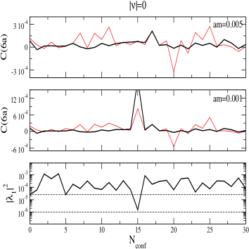
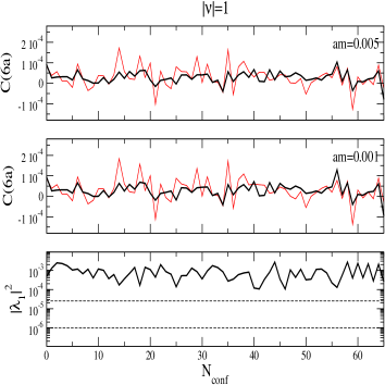
Figure 3: Monte Carlo histories (Lattice B) for the absolute value squared of the lowest non-zero eigenvalue of $D$ (bottom) and for the left-left correlators computed at $t/a=6$: $|\nu|=0$ (left) and $|\nu|=1$ (right), $am=0.001$ (middle) and $am=0.005$ (top). The dashed lines in the eigenvalue plots indicate the two values of $(am)^{2}$. In the plots of the correlation functions, the thick lines are obtained with LMA, while the thin ones in the standard manner.

The values of $F_{P}$ follow a remarkable linear behaviour in the quark mass. A linear fit of the form $aF_{P}=A_{1}+A_{2}\cdot(am)$ gives

$$A_{1}=0.0318(7)\;\,\,, A_{2}=0.093(6)\qquad\,\;\mbox{LMA}$$ (33)

$$A_{1}=0.0310(10)\,, A_{2}=0.100(10)\qquad\mbox{Local}\;.$$ (34)

Quadratic fits to the data give results very well compatible with the previous ones, with the coefficients of the quadratic terms compatible with zero.
Lattice B has been reserved for the $\varepsilon$-regime: we have generated $203$ independent gauge configurations of which 31, 66 and 44 have topological charge $|\nu|=0,\,1,\,2$, respectively. In these topological sectors we have computed the quark propagators for masses $am=0.001,0.005,0.010$ which correspond to $m\Sigma V\approx 0.11,\,0.55,\,1.1$ respectively, if the bare quark condensate $\Sigma$ is taken from the analogous lattice of Ref. [15]. As in the previous case, the two-point correlators of the left-handed current have been computed in the standard manner and with LMA.
In Fig. 3 the Monte Carlo histories for the left-left correlator at $t/a=6$ and for the lowest non-zero eigenvalue of $D^{\dagger}D$ are reported for $|\nu|=0,1$ and $am=0.005,\,0.001$. For the lightest mass, a spike in $C(t)$ is clearly visible in correspondence with a very low (the lowest produced) eigenvalue, which happens to be roughly one order of magnitude lower than its expectation value [15]. A closer look at this configuration reveals that the spiky contribution is indeed due to the light-light contribution $C^{ll}(t)$ and is not cured with the LMA procedure proposed here.

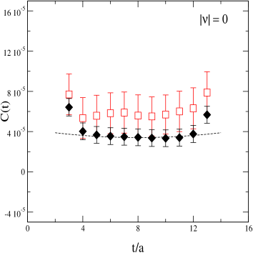
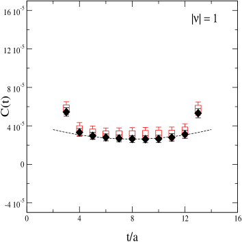
Figure 4: Left-left correlators in the $\epsilon$-regime for $am=0.005$, $|\nu|=0$ (left) and $|\nu|=1$ (right), computed with LMA (filled diamonds) and in the standard manner (open squares). The dashed lines represent fits to LMA data (see main text).

As expected (cf. Sect. 3), for $m\ll 1/\Sigma V$ the Monte Carlo history shows evidence for extreme statistical fluctuations, and therefore we discard data at the lightest mass in the following analysis. The spiky behaviour disappears for the two heavier masses and for them the Monte Carlo history is well-behaved.
For masses $m\sim 1/\Sigma V$, the LMA estimate of the correlation function $C(t)$ is indeed less fluctuating than the one computed in the standard manner. Its variance turns out to be roughly a factor two smaller for the topologies and masses that we consider, as shown in Fig. 4 for $|\nu|=0,1$ and $am=0.005$. The variance reduction is a function of the number of eigenvalues extracted $n$, and the precision $\omega_{k}$ they have been computed with. It can also vary depending on which contributions are chosen to be averaged over. We tried several values of $n$ and $\omega_{k}$ and the ones used in this computation turn out to be a good compromise between the gain in statistics and the additional computational cost (roughly a factor 2), which is mainly due to the computation of the mixed contribution $C^{hl}(t)$. A more systematic optimization of these parameters is desirable but goes beyond the scope of this paper.
We fitted the LMA correlations with the expression given in Eq. (12),

$$C(t)=\frac{B_{1}^{2}}{2T}\,\Big{[}1+B_{2}\,h_{1}\left(\frac{t}{T}\right)\Big{]}\,,$$ (35)

for each topological sector and mass. The lower temporal limit was fixed at $t/a=5$, a point where we found stabilization of the $\chi^{2}$ for all correlators. The results obtained and the associated errors computed with a jackknife procedure are reported in Table 2.

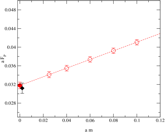
Figure 5: Results obtained in the $p$-regime for $F_{P}$ (open circles) and in the $\epsilon$-regime for $F$ (filled diamond). The dashed line represents a linear fit to the $p$-regime points. The corresponding intercept is also shown (filled circle).

$am$	$|\nu|$		$B_{1}$		$B_{2}$
	0		0.033(3)		3(2)
0.010	1		0.032(2)		5(1)
	2		0.030(2)		5(1)
	0		0.034(4)		2(2)
0.005	1		0.032(2)		4(1)
	2		0.030(2)		4(1)

Table 2: Results from the $\epsilon$-regime data of a fit of the form given in Eq. (35).

Within the large statistical errors, the values for $B_{2}$ are compatible with the prediction of Eq. (12) and the estimate of the condensate extracted in Ref. [15]. The results for $B_{1}$ are very well compatible for all masses and topological sectors. We estimate our best value of the decay constant in the $\epsilon$-regime, $aF=0.0312(11)$, by averaging the two values of $B_{1}$ in each topological sector and then averaging the results as independent determinations. This value is in very good agreement with the linearly extrapolated value from the $p$-regime, as shown in Fig. 5, and constitutes one of the main results of this paper.
By renormalizing the local left-handed current with $Z_{J}=1.55$ [42] and by fixing the lattice spacing with $r_{0}$ from Ref. [46], we obtain $F=104(2)$ MeV and $F=102(4)$ MeV in the $p$ and $\epsilon$-regimes, respectively. These values are compatible within 2$\sigma$ yet more precise than the one we found recently in Ref. [16] from a study of the topological zero-mode wave functions. Note however that the systematic error due to the finite lattice spacing has not been quantified in the present study. The agreement between these two determinations would provide a further check of our main working assumption that quenched ChPT describes the low-energy regime of quenched QCD in certain ranges of kinematical scales. By fitting $F_{P}$ linearly as a function of $(M^{V}_{P})^{2}$, we also obtain our estimate of the LEC in Eq. (11) to be $\alpha_{5}=1.66(8)$. This value is in the same ballpark as the one found in Ref. [47], while it is higher than the one obtained in Ref. [35]. To understand the discrepancy we have analyzed our data as suggested in Ref. [35], and we have found $\alpha_{5}=1.08(5)$, which agrees well with their value of $0.99(6)$. Closer inspection shows that the difference can be traced back to two features of the analysis presented in [35]: the first is the Taylor expansion of $1/(1+\alpha_{5}y_{\mbox{\scriptsize ref}}/2)$ to leading order in $\alpha_{5}$. Although such an expansion is justified, since the difference with the exact result is a higher-order effect, the resulting ambiguity is large and produces an estimate for $\alpha_{5}$ which is smaller by 20–25%. Indeed, this discrepancy was included as a systematic uncertainty in [35]. The remaining difference can be explained by the fact that in Ref. [35] the value $F$ was constrained to coincide with the experimental value of the pion decay constant, which is smaller by about 15% than typical quenched estimates. This assumption is not in accord with our working hypothesis that quenched data should be reproduced by quenched ChPT.
The errors quoted above for the LECs include only our statistical errors. A more detailed assessment of the various systematic errors would require computations at different volumes and lattice spacings, which goes beyond the scope and primary goal of this study.

5 Conclusions

The low-mode averaging technique proposed in this paper reduces large statistical fluctuations in correlation functions due to the presence of local “bumps” in the wave functions associated with the low-lying eigenmodes of the Dirac operator. When applied to the two-point function of the left-handed vector current in the region of quark masses $m\sim 1/\Sigma V$, it provides an estimate of the correlator with a variance significantly reduced with respect to the standard one. As a result the $\epsilon$-regime of QCD can be safely reached in all topological sectors.
It is conceivable that more involved correlation functions such as singlet diagrams (see for example [49]) or those needed for non-leptonic weak decays can also benefit from low-mode averaging. Conventional formulations of lattice QCD may profit as well from this technique. For instance, it could mitigate the problem of exceptional configurations encountered for Wilson fermions, or speed up unquenched simulations.
By matching the quenched QCD results for the left-left correlators computed for quark masses in the $p$- and $\epsilon$-regimes with those of quenched ChPT, we obtained estimates for the quenched low-energy constants $F$ and $\alpha_{5}$. The agreement we found between the value of the pseudoscalar decay constant extrapolated from the $p$-regime and the one extracted directly in the $\epsilon$-regime is remarkable.
In Ref. [16], we studied the possibility of using the contribution of topological zero-mode wave functions to the pseudoscalar correlator, in order to extract $F$. As far as the convergence of the chiral expansion is concerned, it was found that in full QCD (assuming $F\approx 93$ MeV), one would need to go to a lattice extent $\mathop{\raise 1.29167pt\hbox{$>$\kern-7.5pt\raise-4.73611pt\hbox{$\sim$}}}2.0$ fm ($\mathop{\raise 1.29167pt\hbox{$>$\kern-7.5pt\raise-4.73611pt\hbox{$\sim$}}}2.5$ fm) to have the first non-trivial relative correction to be less than 50% (30%). Inspecting the constant part of the $\epsilon$-regime expression in Eq. (7), we find that for the observable studied in the present paper, the same relative corrections would be obtained already with lattice extents $\mathop{\raise 1.29167pt\hbox{$>$\kern-7.5pt\raise-4.73611pt\hbox{$\sim$}}}1.4$ fm ($\mathop{\raise 1.29167pt\hbox{$>$\kern-7.5pt\raise-4.73611pt\hbox{$\sim$}}}1.8$ fm). Therefore, current correlators near the chiral limit should allow for smaller systematic uncertainties in the extraction of the LEC $F$ at realistically accessible volumes than the zero-mode wave functions. It would be interesting to study whether the same remains true for other LECs as well, such as those related to weak decays.
In the quenched theory, on the other hand, systematic errors are very hard to quantify, but the apparent convergence of our expression for the current correlator compares well with the one observed for the zero-mode wave functions in Ref. [16], while having at the same time the advantage that the singlet parameters $m_{0}^{2}/2N_{c}$, $\alpha/2N_{c}$ of quenched chiral perturbation theory do not enter at all at this order.

Appendix A. Some definitions for the GW fermions

In this paper we employ the same conventions as in Ref. [23]. The Dirac matrices satisfy

$$(\gamma_{\mu})^{\dagger}=\gamma_{\mu},\qquad\{\gamma_{\mu},\gamma_{\nu}\}=2\delta_{\mu\nu},$$ (36)

and we have chosen a chiral representation with

$$\gamma_{5}=\gamma_{0}\gamma_{1}\gamma_{2}\gamma_{3}=\pmatrix{1&0\cr 0&-1\cr}.$$ (37)

The chiral projectors are defined as

$$P_{\pm}=\frac{1}{2}(1\pm\gamma_{5})\,.$$ (38)

The Wilson-Dirac operator is given by

$$D_{\rm w}=\frac{1}{2}\left\{\gamma_{\mu}(\nabla^{*}_{\mu}+\nabla_{\mu})-a\nabla^{*}_{\mu}\nabla_{\mu}\right\},$$ (39)

where

$$\nabla_{\mu}\psi(x) = \frac{1}{a}\left\{U(x,\mu)\psi(x+a\hat{\mu})-\psi(x)\right\}\,,$$ (40)

$$\nabla^{*}_{\mu}\psi(x) = \frac{1}{a}\left\{\psi(x)-U(x-a\hat{\mu},\mu)^{-1}\psi(x-a\hat{\mu})\right\}$$ (41)

are the gauge-covariant forward and backward difference operators, $a$ denotes the lattice spacing, $U(x,\mu)\in{\rm SU(3)}$ are the link variables and $\hat{\mu}$ is the unit vector along the direction $\mu$. The Neuberger-Dirac operator is defined as [28]

$$D = \frac{1}{\bar{a}}\left\{1+\gamma_{5}\,\mbox{sign}(Q)\right\},$$ (42)

$$Q = \gamma_{5}\left(aD_{\rm w}-1-s\right),\qquad\bar{a}=\frac{a}{1+s},$$ (43)

where $s$ is a real parameter in the range $|s|<1$. It satisfies the Ginsparg-Wilson relation in Eq. (14). Infinitesimal chiral transformations of the fermion field are given by [29]

$$\delta\psi=\gamma_{5}(1-\bar{a}D)\psi\,,\qquad\delta\bar{\psi}=\bar{\psi}\gamma_{5}\;.$$ (44)

The modified fermion field

$$\tilde{\psi}=(1-\frac{1}{2}\bar{a}D)\psi$$ (45)

transforms according to

$$\delta\tilde{\psi}=\gamma_{5}\tilde{\psi}\,,$$ (46)

and therefore if a composite operator is defined using $\tilde{\psi}$ instead of $\psi$, it has the same transformation behaviour as the corresponding one in the continuum.

Appendix B. Pseudoscalar mass in the $p$-regime of ChPT to NLO

For completeness we report in this appendix NLO expressions for the pseudoscalar meson mass in the $p$-regime of ChPT. We again consider the case of degenerate light quarks only. The effective finite-volume pion mass $M_{P}^{V}$, entering the prediction for the correlation function of two left currents reported in Eq. (4), is given by

$$M_{P}^{V}\equiv M_{P}\biggl{(}1+\frac{g_{1}}{2N_{\rm f}F_{P}^{2}}\biggr{)}\;,$$ (47)

where at the same order the infinite-volume mass $M_{P}$ is

$$M_{P}=M\biggl{[}1+\frac{G(M^{2})}{2N_{\rm f}F^{2}}-\frac{M^{2}}{2(4\pi F)^{2}}\Bigl{(}N_{\rm f}\alpha_{4}+\alpha_{5}-2N_{\rm f}\alpha_{6}-2\alpha_{8}\Bigr{)}\biggr{]}\;.$$ (48)

The function $g_{1}$ reads [48]

$$g_{1}=\frac{1}{(4\pi)^{2}}\int_{0}^{\infty}\frac{{\rm d}\lambda}{\lambda^{2}}e^{-\lambda M_{P}^{2}}\sum_{n\in\mbox{\raisebox{-0.60275pt}{$\scriptstyle\mathsf{ZZ}^{4}$}}}\Bigl{(}1-\delta^{(4)}_{n,0}\Bigr{)}\exp\Bigl{[}-\frac{1}{4\lambda}\Bigl{(}T^{2}n_{0}^{2}+L^{2}\sum_{i=1}^{3}n_{i}^{2}\Bigr{)}\Bigr{]}\;,$$ (49)

and, in dimensional regularization ,

$$G(M^{2})=\int\frac{{\rm d}^{d}p}{(2\pi)^{d}}\frac{1}{p^{2}+M^{2}}\;.$$ (50)

In the quenched approximation (to the extent that it is well defined for this observable), these predictions are modified to be

$$M_{P}^{V}=M_{P}\biggl{[}1+\frac{1}{2F_{P}^{2}}\biggl{(}\frac{\alpha}{2N_{c}}+\frac{\alpha M_{P}^{2}-m_{0}^{2}}{2N_{c}}\frac{{\rm d}}{{\rm d}M_{P}^{2}}\biggr{)}g_{1}\,\biggr{]}\;,$$ (51)

with the infinite-volume mass $M_{P}$ given by

$$M_{P}=M\biggl{[}1+\frac{1}{2F^{2}}\biggl{(}\frac{\alpha}{2N_{c}}G(M^{2})+\frac{m_{0}^{2}-\alpha M^{2}}{2N_{c}}H(M^{2})\biggr{)}-\frac{M^{2}}{2(4\pi F)^{2}}(\alpha_{5}-2\alpha_{8})\biggr{]}\;.$$ (52)

In Eqs. (51) and (52), $\alpha/2N_{c}$ and $m_{0}^{2}/2N_{c}$ are the parameters related to the flavour singlet field (with the normalisation conventions of [34, 37]), and

$$H(M^{2})=\int\frac{{\rm d}^{d}p}{(2\pi)^{d}}\frac{1}{(p^{2}+M^{2})^{2}}\;.$$ (53)

References

- [1] S. Weinberg, Physica A 96 (1979) 327.
- [2] J. Gasser and H. Leutwyler, Annals Phys. 158 (1984) 142; Nucl. Phys. B 250 (1985) 465.
- [3] F. Butler, H. Chen, J. Sexton, A. Vaccarino and D. Weingarten, Nucl. Phys. B 430 (1994) 179.
- [4] S. Aoki et al. [CP-PACS Collaboration], Phys. Rev. D 67 (2003) 034503.
- [5] P. Hasenfratz, S. Hauswirth, T. Jörg, F. Niedermayer and K. Holland, Nucl. Phys. B 643 (2002) 280.
- [6] C. Gattringer et al. [BGR Collaboration], Nucl. Phys. B 677 (2004) 3.
- [7] C. Bernard et al., Nucl. Phys. Proc. Suppl. 119 (2003) 170.
- [8] S. J. Dong et al., arXiv:hep-lat/0304005.
- [9] J. Gasser and H. Leutwyler, Phys. Lett. B 188 (1987) 477; Nucl. Phys. B 307 (1988) 763.
- [10] H. Neuberger, Phys. Rev. Lett. 60 (1988) 889; Nucl. Phys. B 300 (1988) 180.
- [11] P. H. Damgaard, R. G. Edwards, U. M. Heller and R. Narayanan, Phys. Rev. D 61 (2000) 094503.
- [12] P. Hernández, K. Jansen and L. Lellouch, Phys. Lett. B 469 (1999) 198; P. Hernández, K. Jansen, L. Lellouch and H. Wittig, JHEP 07 (2001) 018; T. DeGrand [MILC Collaboration], Phys. Rev. D 64 (2001) 117501.
- [13] S. Prelovsek and K. Orginos [RBC Collaboration], Nucl. Phys. Proc. Suppl. 119 (2003) 822; K.I. Nagai, W. Bietenholz, T. Chiarappa, K. Jansen and S. Shcheredin, arXiv:hep-lat/0309051; T. Chiarappa, W. Bietenholz, K. Jansen, K.I. Nagai and S. Shcheredin, arXiv:hep-lat/0309083; W. Bietenholz, T. Chiarappa, K. Jansen, K.I. Nagai and S. Shcheredin, arXiv:hep-lat/0311012;
- [14] W. Bietenholz, K. Jansen and S. Shcheredin, JHEP 07 (2003) 033.
- [15] L. Giusti, M. Lüscher, P. Weisz and H. Wittig, JHEP 11 (2003) 023.
- [16] L. Giusti, P. Hernández, M. Laine, P. Weisz and H. Wittig, JHEP 01 (2004) 003.
- [17] H. Leutwyler and A. Smilga, Phys. Rev. D 46 (1992) 5607.
- [18] E. V. Shuryak and J. J. Verbaarschot, Nucl. Phys. A 560 (1993) 306; J. J. Verbaarschot and I. Zahed, Phys. Rev. Lett. 70 (1993) 3852; J. J. Verbaarschot, Phys. Rev. Lett. 72 (1994) 2531.
- [19] S. M. Nishigaki, P. H. Damgaard and T. Wettig, Phys. Rev. D 58 (1998) 087704; P. H. Damgaard and S. M. Nishigaki, Phys. Rev. D 63 (2001) 045012.
- [20] G. Akemann and P. H. Damgaard, Phys. Lett. B 583 (2004) 199.
- [21] R. G. Edwards, U. M. Heller, J. E. Kiskis and R. Narayanan, Phys. Rev. Lett. 82 (1999) 4188; Phys. Rev. D 61 (2000) 074504.
- [22] R. G. Edwards, Nucl. Phys. Proc. Suppl. 106 (2002) 38 and references therein.
- [23] L. Giusti, C. Hoelbling, M. Lüscher and H. Wittig, Comput. Phys. Commun. 153 (2003) 31.
- [24] P. H. Ginsparg and K. G. Wilson, Phys. Rev. D 25 (1982) 2649.
- [25] D. B. Kaplan, Phys. Lett. B 288 (1992) 342.
- [26] R. Narayanan and H. Neuberger, Phys. Lett. B 302 (1993) 62; Phys. Rev. Lett. 71 (1993) 3251; Nucl. Phys. B 412 (1994) 574 and B 443 (1995) 305.
- [27] Y. Shamir, Nucl. Phys. B 406 (1993) 90; V. Furman and Y. Shamir, Nucl. Phys. B 439 (1995) 54.
- [28] H. Neuberger, Phys. Lett. B 417 (1998) 141; Phys. Rev. D 57 (1998) 5417; Phys. Lett. B 427 (1998) 353.
- [29] M. Lüscher, Phys. Lett. B 428 (1998) 342.
- [30] P. Hernández, K. Jansen and M. Lüscher, Nucl. Phys. B 552 (1999) 363.
- [31] T. DeGrand and S. Schaefer, arXiv:hep-lat/0401011.
- [32] C. W. Bernard and M.F.L. Golterman, Phys. Rev. D 46 (1992) 853.
- [33] S. R. Sharpe, Phys. Rev. D 46 (1992) 3146.
- [34] P. Hernández and M. Laine, JHEP 01 (2003) 063.
- [35] J. Heitger, R. Sommer and H. Wittig [ALPHA Collaboration], Nucl. Phys. B 588 (2000) 377.
- [36] F. C. Hansen, Nucl. Phys. B 345 (1990) 685; F. C. Hansen and H. Leutwyler, Nucl. Phys. B 350 (1991) 201.
- [37] P. H. Damgaard, P. Hernández, K. Jansen, M. Laine and L. Lellouch, Nucl. Phys. B 656 (2003) 226.
- [38] R. Brower, P. Rossi and C. I. Tan, Nucl. Phys. B 190 (1981) 699.
- [39] L. Del Debbio and C. Pica, JHEP 02 (2004) 003.
- [40] G. Colangelo and E. Pallante, Nucl. Phys. B 520 (1998) 433.
- [41] J.C. Osborn, D. Toublan and J.J. Verbaarschot, Nucl. Phys. B 540 (1999) 317; P.H. Damgaard, J.C. Osborn, D. Toublan and J.J. Verbaarschot, Nucl. Phys. B 547 (1999) 305.
- [42] L. Giusti, C. Hoelbling and C. Rebbi, Phys. Rev. D 64 (2001) 114508, Erratum-ibid. D 65 (2002) 079903; L. Giusti, C. Hoelbling and C. Rebbi, Nucl. Phys. Proc. Suppl. 106 (2002) 739.
- [43] P. Hernández, K. Jansen, L. Lellouch and H. Wittig, Nucl. Phys. Proc. Suppl. 106 (2002) 766.
- [44] P. Hernández, Nucl. Phys. Proc. Suppl. 106 (2002) 80.
- [45] L. Giusti, Nucl. Phys. Proc. Suppl. 119 (2003) 149.
- [46] S. Necco and R. Sommer, Nucl. Phys. B 622 (2002) 328.
- [47] W. A. Bardeen, E. Eichten and H. Thacker, arXiv:hep-lat/0307023.
- [48] P. Hasenfratz and H. Leutwyler, Nucl. Phys. B 343 (1990) 241.
-
[49]
H. Neff, N. Eicker, T. Lippert, J. W. Negele and K. Schilling,
Phys. Rev. D 64 (2001) 114509.
T. DeGrand and U. M. Heller [MILC collaboration], Phys. Rev. D 65 (2002) 114501.
C. McNeile and C. Michael [UKQCD Collaboration], arXiv:hep-lat/0402012.