$N_{f}=1$ QCD simulation with improved gauge action at finite temperature

Abstract

We study the deconfinement transition of $N_{f}=1$ QCD by the hybrid Monte Carlo algorithm with Wilson fermions. We calculate the Polyakov loop, its susceptibility and Binder cumulant and use the $\chi^{2}$ method to locate the phase transition point. Our results are similar to the previous results obtained by the multiboson algorithm.

1 Introduction

Lüscher proposed the multiboson algorithm[1, 2] in which a polynomial approximation to the inverse of the fermion matrix is used. This algorithm is considered to be an alternative one to simulate dynamical QCD. Boriçi and de Forcrand[3] noticed that the polynomial approximation can be used to simulate odd flavour QCD. Then the multiboson algorithm is used to study the deconfinement transition in one flavour QCD[4]. The original hybrid Monte Carlo (HMC) algorithm[5] is limited for even flavour case. However the polynomial approximation can be also applied for the HMC[6], which means that one can also simulate odd flavour QCD by the HMC[7]. We investigate the phase structure of one flavour QCD by the HMC and check whether different algorithms give the same results. We calculate Polyakov loop, its susceptibility and Binder cumulant and use the $\chi^{2}$ method[8] to locate the precise position of the phase transition. Mainly we present results from the Wilson gauge action, and also give preliminary results from the DBW2 gauge action[9].

2 $N_{f}=1$ algorithm

The partition function of $N_{f}=1$ QCD is given by $\displaystyle Z=\int[dU]\det D\exp(-S_{g}[U]).$ One can approximate the inverse of $D$ by a polynomial[1] as $\displaystyle 1/D\approx P_{m}(D)\equiv\prod_{k=1}^{m}(D-z_{k}),$ where $z_{k}$ are the roots of the polynomial $P_{m}(D)$. For the even degree $m$, det$D$ can be rewritten as

$$\mathrm{det}D=C_{n}\mathrm{det}(T^{\dagger}_{n}(D)T_{n}(D))^{-1},$$ (1)

where $T_{n}(D)\equiv\prod_{k=1}^{n}(D-Z_{2k-1})$, and $C_{n}\equiv\mathrm{det}(DT_{n}^{\dagger}(D)T_{n}(D))^{-1}$ is a correction factor to the polynomial approximation. det$(T_{n}^{\dagger}(D)T_{n}(D))$ can be expressed as,

$$\mathrm{det}(T_{n}^{\dagger}(D)T_{n}(D))^{-1}$$ (2)

$$\approx \int[d\phi^{\dagger}][d\phi]\mathrm{exp}(-\phi^{\dagger}T_{n}^{\dagger}(D)T_{n}(D)\phi).$$

Then one can define $N_{f}=1$ Hamiltonian for HMC algorithm as,

$$H^{N_{f}=1}=\frac{1}{2}\sum_{i}P_{i}^{2}+S_{g}[U]+\phi^{\dagger}T_{n}^{\dagger}(D)T_{n}(D)\phi.$$ (3)

where $P_{i}$ are momenta which are conjugate to link variables. $\phi^{\dagger}T_{n}^{\dagger}(D)T_{n}(D)\phi$ is manifestly positive, which is essential to the implementation of the HMC. The correction factor $C_{n}$ is used to make the algorithm exact[7].

$\kappa$	$8^{3}\times 4$		$12^{3}\times 4$		$16^{3}\times 4$
	$n$/Acc	traj.	$n$/Acc	traj.	$n$/Acc	traj.
0.05	8/0.86	10K	12/0.75	12K	24/0.62	12K
0.10	16/0.86	10K	24/0.74	12K	32/0.62	12K
0.12	24/0.86	15K	32/0.75	20K	40/0.62	14K
0.14	32/0.86	10K	40/0.74	14K	50/0.61	12K

Table 1: $n$ and Acc are the number of degrees of polynomial and acceptance ratio of the HMC respectively. The step size $d\tau$ is set to $0.05$ for all simulations. To obtain the best performance of the HMC one should tune $d\tau$ so that the acceptance is $60-70\%$[10]. In this study we have not done such tuning.

3 $\chi^{2}$–method

In this study we use $\chi^{2}$–method[8] to find critical $\beta$ for each $\kappa$. By differentiating the singular part of the free energy density on $N_{s}^{3}\times N_{t}$ lattice and expanding these equations with respect to $x$, we obtain the leading $N_{s}$ behavior at $x=0$,

$$\ln\langle L\rangle(x=0,N_{s}) = c_{0}\ln N_{s}+c_{1},$$ (4)

$$\ln\chi(x=0,N_{s}) = c_{0}\ln N_{s}+c_{1},$$ (5)

$$B_{4}(x=0,N_{s}) = c_{0}+c_{1}N_{s}^{-\omega}.$$ (6)

where $\langle L\rangle$, $\chi$, $B_{4}$ and $x$ are Polyakov loop, its susceptibility, Binder cumulant[11] and reduced temperature $(T-T_{c})/T_{c}$ respectively:

$$L = \frac{1}{N_{s}^{3}}\sum_{x}\frac{1}{N}\mbox{Tr}\prod_{t}U_{4}(x,t)$$ (7)

$$\chi = N_{s}^{3}(\langle L^{2}\rangle-\langle L\rangle^{2}),~{}~{}~{}\chi_{v}=N_{s}^{3}\langle L^{2}\rangle,$$ (8)

$$B_{4} = \frac{\langle L^{4}\rangle}{{\langle L^{2}\rangle}^{2}}-3$$ (9)

The critical point can be obtained at the point where a fit to the leading $N_{s}$-behavior has the least $\chi^{2}$[8].

4 Simulations

We perform numerical simulation using the hybrid Monte Carlo (HMC) with polynomial approximation[7]. We use the Wilson and DBW2[9] gauge actions. Lattice gauge action is given by

$$S_{g}[U]=\frac{\beta}{3}((1-8c_{1})\sum\mathrm{ReTr}W_{11}+c_{1}\sum\mathrm{ReTr}W_{12})$$ (10)

where $W_{11}$ and $W_{12}$ stand for $1\times 1$ and $1\times 2$ Wilson loop. For Wilson action the coefficient is set to $c_{1}=0$ and $c_{1}=-1.4089$ for DBW2 action.

To obtain values of observables at different $\beta$ from a single simulation, we use the re-weighting method[12]. Statistical errors are evaluated by the Jackknife method.

5 Results

In Fig.1 we show the volume dependence of peak of Polyakov loop susceptibility, which is expected to behave as $V^{\alpha}$. The behavior is similar to the previous results[4], i.e. $\alpha$ decreases as $\kappa$ increases. However the precise values of $\alpha$ are slightly different from the previous ones, which may indicate that our statistics is not enough to conclude.

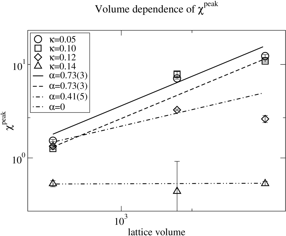
Figure 1: Volume dependence of peak of Polyakov loop susceptibility.

We summarize results for $\beta_{c}$ from $|L|$, $\chi_{v}$ and $B_{4}$ in Table.2.

$\kappa$	$\beta_{c}^{|L|}$	$\beta_{c}^{\chi_{v}}$	$\beta_{c}^{B_{4}}$
0.05	5.674(4)	5.672(3)	5.685(6)
0.10	5.676(5)	5.674(4)	5.680(2)
0.12	5.630(1)	5.631(2)	5.631(1)
0.14	5.595(2)	5.592(2)	5.616(6)

Table 2: Preliminary results of critical $\beta$ from various observables. $\beta_{c}^{|L|}$, $\beta_{c}^{\chi_{v}}$ and $\beta_{c}^{B_{4}}$ stand for critical $\beta$ from Polyakov loop, $\chi_{v}$ and $B_{4}$ respectively.

We estimated the critical $\beta$ using the $\chi^{2}$-method. The data were fitted to Eq.(4)– Eq.(6). For Eq.(6) $\omega$ was fixed to $1$ in accordance with [8]. As an example in Fig.2 $\chi^{2}/N_{fit}$ curve at $\kappa=0.12$ is shown. Here $N_{fit}$ is the degrees of freedom for the fitting. We determine $\beta_{c}$ at the minimum point of the $\chi^{2}/N_{fit}$ curve.

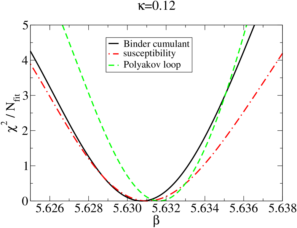
Figure 2: $\chi^{2}/N_{fit}$ curves at $\kappa=0.12(\beta=5.630)$. $N_{fit}=2$.

$\beta_{c}^{|L|}$, $\beta_{c}^{\chi_{v}}$ and $\beta_{c}^{B_{4}}$ should coincide with each other. However we observed that at $\kappa=0.05,0.10$ and $0.14$ $\beta_{c}^{B_{4}}$ is slightly different from others. This might be due to less statistics. To determine $\beta_{c}$ precisely more statistics is needed.

The results with DBW2 gauge action ( quenched and $\kappa=0.1$ ) are shown in Fig.3. We are currently performing simulations at other $\kappa$.

Figure 3: Plaquette susceptibility from quenched and full QCD simulations with DBW2 gauge action. The full QCD simulation is performed at $\kappa=0.10$.

References

- [1] M.Luscher, Nucl. Phys. B 418 (1994) 637.
- [2] A. Borrelli,Ph. de Forcrand and A. Galli, Nucl.Phys. B 477 (1996) 809.
- [3] A. Boriçi and Ph. de Forcrand, Nucl. Phys. B 454 (1995) 645.
- [4] C. Alexandrou, A. Boriçi, A. Feo, Ph. de Forcrand, A. Galli, F. Jegerlehner and T. Takaishi, Phys.Rev. D 60 (1999) 034504; Nucl. Phys. Proc. Suppl. 63 (1998) 406.
- [5] S.Duane, A.Kennedy, B.Pendleton and D.Roweth, Phys. Lett. B 195 (1987) 216.
- [6] Ph. de Forcrand and T. Takaishi, Nucl. Phys. Proc. Suppl. 53 (1997) 968.
- [7] T. Takaishi and Ph. de Forcrand, Int.J.Mod.Phys. C 13 (2002) 343; Nucl. Phys. Proc. Suppl. 94 (2001) 818; arXiv:hep-lat/0009024.
- [8] J.Engels, S.Mashkevich, T.Scheideler, G.Zinovjev, Phys.Lett. B 365 (1996) 219.
- [9] T.Takaishi, Phys.Rev. D 54 (1996) 1050; T.Takaishi and Ph. de Forcrand, Phys.Lett. B 428 (1998) 157; Ph. de Forcrand et.al., Nucl.Phys.B577 (2000) 263.
- [10] T. Takaishi, Comput. Phys. Commun. 133 (2000) 6; Phys. Lett. B 540 (2002) 159.
- [11] K.Binder, Z.Phys. B 43 (1981) 119.
- [12] A. M. Ferrenberg and R. H. Swendsen, Phys. Rev. Lett. 63 (1989) 1195.