ITP-Budapest 606
WUB 04-02
The QCD equation of state at finite $T/\mu$ on the lattice

Abstract

We present $N_{t}=4$ lattice results for the equation of state of  $2+1$ flavour staggered, dynamical QCD at finite temperature and chemical potential. We use the overlap improving multi-parameter reweighting technique to extend the equation of state for non-vanishing chemical potentials. The results are obtained along the line of constant physics. Our physical parameters extend in temperature and baryon chemical potential upto $\approx 500-600$ MeV.

1 Introduction

QCD at finite $T$ and/or $\mu$ is of special importance since it can be used to describe the early universe, neutron stars and also heavy ion collisions. Present and future heavy ion collisions are carried out at CERN, in Brookhaven and at GSI to detect and study experimentally the QGP phase, i.e. QCD at large temperature and moderate chemical potentials [1, 3]. It is very important to understand the theoretical grounds of the underlying physics. First principle answers can be gained from lattice QCD calculations e.g. to obtain the equation of state (EoS).

The experiments are carried out at $\mu\neq 0$ but unfortunately until recently the lattice results were limited to $\mu=0$. Though lattice QCD can be easily formulated at non-vanishing chemical potentials [4, 5] we cannot use Monte-Carlo simulations at $\mu\neq 0$ as the determinant of the Euclidean Dirac operator and so the functional measure becomes complex.

Recently two of us proposed a new technique [6], the so-called overlap improving multi-parameter reweighting method to study lattice QCD at finite $\mu$ . This procedure proved to be good enough to give the phase boundary on the $T$-$\mu$ plane for four flavours [6], for 2+1 flavours [7] and the equation of state [8, 9]. Essentially the same technique was used succesfully by other studies [10, 11, 12]; however, instead of evaluating the fermionic determinant exactly it can be approximated by its Taylor series with respect to $\mu$. Other approaches, like simulations at imaginary chemical potential and analytic continuation led to results that are in good agreement with those of our method [13, 14, 15].

In this paper we determine the EoS on the line of constant physics (LCP). An LCP can be defined by a fixed ratio of the strange quark mass ($m_{s}$) and the light quark masses ($m_{u}d$) to the $\mu=0$ transition temperature ($T_{c}$). Our parameter choice approximately corresponds to the physical strange quark mass. However, the ratio of the pion mass ($m_{\pi}$) and the rho mass ($m_{\rho}$) is around 0.5-0.75, which is roughly 3 times larger than its physical value. In our lattice analysis we use $2+1$ flavour QCD with dynamical staggered quarks. The determination of the EoS at finite chemical potential needs several observables at non-vanishing $\mu$-s. These are produced by the use of the multi-parameter reweighting method. We employ the integral method to calculate the pressure [16].

The paper is organized as follows. In Section 2 we summarize the lattice parameters and the technique by which the lines of constant physics can be determined. Section 3 presents the equation of state at vanishing chemical potential. Sections 4 deals with the question how to reweight into the region of $\mu\neq 0$ and how to estimate the error of the reweighted quantities. In Section 5 we give the equation of state for non-vanishing chemical potential and temperature. Those who are not interested in the details of the lattice techniques should simply omit Sections 2–4 and jump to Section 5, or refer to [8]. Finally, Section 6 contains a summary and the conclusions. The details of this work can be found in [9].

2 Lattice parameters and the line of constant physics

In this paper we use $2+1$ flavour dynamical QCD with unimproved staggered action. Simulations are done for the equation of state along two different lines of constant physics and at 14 different temperatures. The temperature range spans up to $3T_{c}$. In physical units our parameters correspond to pion to rho mass ratio of $m_{\pi}/m_{\rho}\approx 0.5-0.75$ and lattice spacings of $a\approx 0.12-0.35$ fm.

The finite temperature contributions to the EoS are obtained on $4\cdot 8^{3}$, $4\cdot 10^{3}$ and $4\cdot 12^{3}$ lattices, which can be used to extrapolate into the thermodynamical limit (we usually call them hot lattices). On these lattices we determine not only the usual observables (plaquette, Polyakov line, chiral condensates) but also the determinant of the fermion matrix and the baryon density ($n_{B}$) at finite $\mu$. $10000-20000$ trajectories are simulated at each bare parameter set. Plaquettes, Polyakov lines and the chiral condensates are measured at each trajectories whereas the CPU demanding determinants and related quantities are evaulated at every 30 trajectories. For our parameters the CPU time used for the production of configurations is of the same order of magnitude as the CPU time used for calculating the determinants.

Since we usually move along the line of constant physics by changing the lattice spacing $a$ and keeping the masses fixed we will explicitely write out the lattice spacing $a$ in our formulas. In this paper we study lattices with isotropic couplings. We write $\mu_{B}$ for the baryonic chemical potential, whereas for the quark chemical potential ($u,d$ quarks) we use the notation $\mu$. Similarly, the baryon density is denoted by $n_{B}$ and the light quark density by $n$.

In the remaining part of this section we discuss the role of LCP when determining the EoS in pure gauge theory and in dynamical QCD. After that we determine the lines of constant physics, along which our simulations are done.

In order to detetermine the temperature $T=1/[N_{t}a(\beta)]$ of the pure gauge theory, we have to compute the lattice spacing ($a$) as a function of the gauge coupling ($\beta$). In the $d$ dimensional space of the bare parameters one defines $d$ appropriately chosen quantities. The LCP is given by $d-1$ constraints and it is parametrized by a non-constrained combination of the above quantities. For the $2+1$ flavour staggered action we have three bare parameters ($\beta$, and two masses, $m_{ud},m_{s}$). Thus, we need two constraints. There are several possibilities for these constraints and consequently there are many ways to define an LCP. A convenient choice for two of the three quantities can be the bare quark masses ($m_{ud}$ and $m_{s}$). A more physical possibility is to use the pion and kaon masses ($m_{\pi},m_{K}$).

In our analysis first we use the bare quark masses ($m_{ud}$ and $m_{s}$) and the transition temperature to define an LCP. In this paper we use two LCP’s (LCP₁ and LCP₂). The conditions

$$\begin{array}[]{c}m_{ud}=0.48T_{c}=0.48/(N_{t}a)\ \ \ \ {\rm and}\ \ \ \ \ m_{s}=2.08\cdot m_{ud}\\ m_{ud}=0.384T_{c}=0.384/(N_{t}a)\ \ \ \ {\rm and}\ \ \ \ \ m_{s}=2.08\cdot m_{ud}\end{array}$$ (3)

are taken as the constraints for LCP₁ and LCP₂, respectively. For both LCP’s we determined four different transition couplings ($\beta_{c}$) by susceptibility peaks on $N_{t}=1/(T_{c}a)=4$, 6, 8 and 10 lattices with spatial extensions $N_{s}\mathop{\raise 1.29167pt\hbox{$>$\kern-7.5pt\raise-4.73611pt\hbox{$\sim$}}}3N_{t}/2$ and quark masses given by eq. (3). The quark masses or the transition gauge couplings can be used to parametrize the LCP’s.

By the finite temperature technique, described above, only a few points of the LCP’s can be obtained. To interpolate $\beta(a)$ between these points (and extrapolate slightly away from them) we use the renormalization group inspired ansatz proposed by Allton [17]. A particularly illustrative parametrization is obtained by inverting eq. (3) and using $N_{t}$ as a continuous parameter. Figure 1 shows LCP₁ and LCP₂ with our simulation points. The simulation points in the “non-LCP” approach – often used in the literature – are also shown. Note that even though the determination of the LCP₁ and LCP₂ are done on finite temperature lattices, the obtained bare parameters are used in the rest of the paper for $T=0$ and $T\neq 0$ simulations.

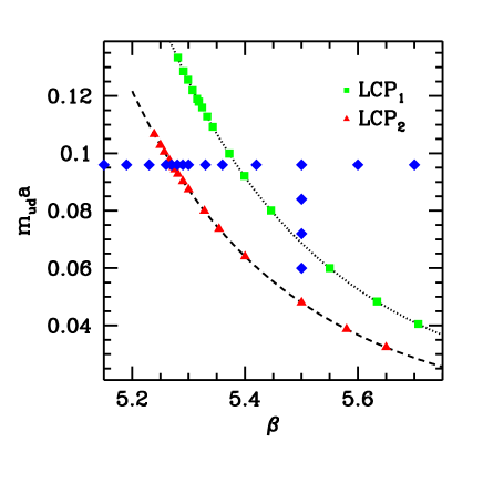
Figure 1: The lines of constant physics (LCP₁ and LCP₂) on the $\beta$ vs. $m_{ud}a$ plane. The strange quark mass is given by $m_{s}=2.08m_{ud}$ for both LCP’s. The simulation points are shown by squares/triangles and connected by dashed/dotted lines for LCP₁/LCP₂, respectively. The diamonds along a horizontal line represent the simulation points in the “non-LCP” approach. Additional 4 diamonds in the vertical direction show the simulation points used to test the path independence of the integral method.

3 Equation of state along the lines of constant physics (LCP) at $\mu=0$

In previous studies of the EoS with staggered quark actions, the pressure and the energy density were determined as functions of the temperature for fixed value of the bare quark mass $m_{q}a$ in the lattice action [18, 19, 20]. In these studies a fixed $N_{t}$ was used (e.g. $N_{t}=4$ or 6) at different temperatures. Since $T=1/(N_{t}a)$ the temperature is set by the lattice spacing which changes with $\beta$. This convenient, fixed bare $m_{q}a$ choice leads to a system which has larger and larger physical quark masses at decreasing lattice spacings (thus, at increasing temperatures). Increasing physical quark masses with increasing temperatures could result in systematic errors of the EoS.

Clearly, instead of this sort of analysis (in the rest of the paper we refer to it as “non-LCP approach”) one intends to study the temperature dependence of a system with fixed physical observables, therefore on an LCP.

In our analysis we use full QCD with staggered quarks along the LCP and compare these results with those of the “non-LCP approach”.

Now, we briefly review the basic formulas and emphasize the issues related to the EoS determination along an LCP.

The energy density and pressure are defined in terms of the free-energy density ($f$):

$$\epsilon(T)=f-T\frac{\partial{f}}{\partial{T}},\ \ \ \ \ \ \ \ p(T)=-f.$$ (4)

Expressing the free energy in terms of the partition function ($f=-T/V\log Z=$
$-T\partial(\log Z)/\partial V$) we have:

$$\epsilon(T)=\frac{T^{2}}{V}\frac{\partial{\log Z}}{\partial{T}},\ \ \ \ \ \ \ \ p(T)=T\frac{\partial(\log Z)}{\partial V}.$$ (5)

The temperature and volume are connected to this lattice spacing by

$$T=\frac{1}{aN_{t}}, V=a^{3}N_{s}^{3}.$$ (6)

Inspecting eqs.(5, 6) we see that $(\epsilon-3p)/T^{4}$ is directly proportional to the total derivative of $\log Z$ with respect to the lattice spacing:

$$\frac{\epsilon-3p}{T^{4}}=-\frac{N_{t}^{3}}{N_{s}^{3}}a\frac{d(\log Z)}{da}.$$ (7)

Here, the derivative with respect to $a$ is defined along the LCP, which means that only the lattice spacing changes and the physics (in our case $m_{q}/T_{c}$) remains the same. We can write:

$$\frac{d}{da}=\frac{\partial\beta}{\partial a}\frac{\partial}{\partial\beta}+\sum_{q}\frac{\partial(m_{q}a)}{\partial a}\frac{\partial}{\partial(m_{q}a)}.$$ (8)

Since the LCP is defined by $m_{q}/T_{c}={\rm const.}$, the partial derivative $\partial(m_{q}a)/\partial a$ becomes simply $m_{q}$. The derivatives of $\log Z$ with respect to $\beta$ and $m_{q}$ are the plaquette and $\bar{\Psi}\Psi_{q}$ averages multiplied by the lattice volume. We get:

$$\frac{\epsilon-3p}{T^{4}}=-N_{t}^{4}a\left(\overline{{\rm Pl}}\left.\frac{\partial\beta}{\partial a}\right|_{\rm LCP}+\sum_{q}\overline{\bar{\Psi}\Psi}_{q}m_{q}\right).$$ (9)

The pressure is usually determined by the integral method [16]. The pressure is simply proportional to $\log Z$, however it cannot be measured directly. One can determine its partial derivatives with respect to the bare parameters. Thus, we can write:

$$\frac{p}{T^{4}}=\left[-\frac{N_{t}^{3}}{N_{s}^{3}}\int^{(\beta,m_{q}a)}_{(\beta_{0},m_{q0}a)}d(\beta,m_{q}a)\left(\begin{array}[]{c}{\partial\log Z}/{\partial\beta}\\ {\partial\log Z}/{\partial(m_{q}a)}\end{array}\right)\right]-\frac{p_{0}}{T^{4}}.$$ (10)

Since the integrand is the gradient of $\log Z$, the result is by definition independent of the integration path (we explicitely checked this path independence). For the substracted vacuum term we used the zero temperature pressure, i.e. the same integral on $N_{t0}=N_{s}$ lattices. The lower limits of the integrations (indicated by $\beta_{0}$ and $m_{q0}$) were set sufficiently below the transition point. By this choice the pressure becomes independent of the starting point (in other words it vanishes at vanishing temperature). In the case of $2+1$ staggered QCD eq. (10) can be rewritten appropriately and the pressure is given by

$$\frac{p}{T^{4}}=-N_{t}^{4}\int^{(\beta,m_{q}a)}_{(\beta_{0},m_{q0}a)}d(\beta,m_{ud}a,m_{s}a)\left(\begin{array}[]{c}\langle{\rm Pl}\rangle\\ \langle\bar{\Psi}\Psi_{ud}\rangle\\ \langle\bar{\Psi}\Psi_{s}\rangle\end{array}\right),$$ (11)

where we use the following notation for subtracting the vacuum term:

$$\langle{\cal O}(\beta,m)\rangle={\overline{{\cal{O}}}(\beta,m)}_{T\neq 0}-{\overline{{\cal O}}(\beta,m)}_{T=0}.$$ (12)

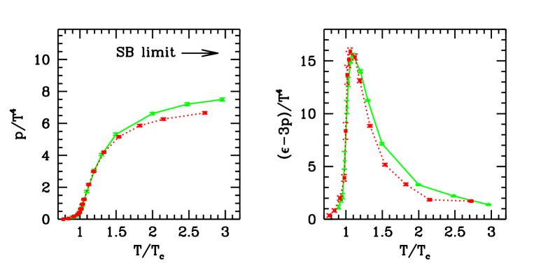
Figure 2: The equation of state at $\mu$=0. (a) The left panel shows the pressure $p$, as a function of the temperature. All quantities are normalised by $T^{4}$. In order to lead the eye the solid line connects the data points obtained along the LCP₂, whereas the dashed line connects the data points obtained in the “non-LCP approach” (see text). The Stefan-Boltzmann limit is also shown by an arrow for $N_{t}$=4 lattices. The EoS along the LCP and the “non-LCP approach” differ from each other at high T. (b) The same for $\epsilon$-3p.

Figure 2 shows the EoS at vanishing chemical potential on $N_{t}=4$ lattices for LCP₂ and for the non-LCP approach. The pressure and $\epsilon-3p$ are presented as a function of the temperature. The parameters of LCP₂ and those of the non-LCP approaches coincide at $T=T_{c}$. The Stefan-Boltzmann limit valid for $N_{t}=4$ lattices is also shown.

It can be seen that the EoS along the LCP and the “non-LCP approach” differ from each other at high temperatures. This is an obvious consequence of the fact that in the “non-LCP approach” the bare quark mass increases linearly with the temperature. The “LCP” pressure is much closer to the SB limit.

4 Reliability of reweighting and the best reweighting lines

The aim of this section is to study the reliability of the multi-parameter reweighting (for another study of reweighting see [21]). We also determine its region of validity by a suitably estimated error. To start with let us briefly review the multi-parameter reweighting.

As proposed in [6] one can identically rewrite the partition function in the form:

$$Z(m,\mu,\beta)=\int{\cal D}U\exp[-S_{bos}(\beta_{0},U)]\det M(m_{0},\mu=0,U)$$ (13)

$$\left\{\exp[-S_{bos}(\beta,U)+S_{bos}(\beta_{0},U)]\frac{\det M(m,\mu,U)}{\det M(m_{0},\mu=0,U)}\right\},$$

where $U$ denotes the gauge field links and $M$ is the fermion matrix . The chemical potential $\mu$ is included as $\exp(a\mu)$ and $\exp(-a\mu)$ multiplicative factors of the forward and backward timelike links, respectively. In this approach we treat the terms in the curly bracket as an observable – which is measured on each independent configuration, and can be interpreted as a weight – and the rest as the measure. Thus the simulation can be performed at $\mu=0$ and at some $\beta_{0}$ and $m_{0}$ values (Monte-Carlo parameter set). By using the reweighting formula (13) one obtains the partition function at another set of parameters, thus at $\mu\neq 0$, $\beta\neq\beta_{0}$ or even at $m\neq m_{0}$ (target parameter set).

Expectation values of observables can be determined by the above technique. In terms of the weights (i.e. the expression in the curly bracket of eq. (13)) the averages can be determined as:

$${\overline{\cal O}}(\beta,\mu,m)=\frac{\sum\{w(\beta,\mu,m,U)\}{\cal O}(\beta,\mu,m,U)}{\sum\{w(\beta,\mu,m,U)\}}.$$ (14)

Now we present an error estimate of the reweighting procedure which also shows how far we can reweight in the target parameter space .

The steps of the new procedure are as follows. First, we assign to each configuration of our initial sample the weight $w$ valid at the chosen target parameter set i.e.

$$w=\exp\left\{\Delta\beta\cdot V\cdot(Pl)+\frac{n_{f}}{4}[\ln\det M(\mu)-\ln\det M(\mu=0)]\right\}$$ (15)

where $V$ is the lattice volume. Next, we carry out Metropolis-like accept/reject steps with the series of these new weights. This procedure generates a new, somewhat smaller, sample. The configurations of this new sample are taken with a unit weight to calculate expectation values, variances and integrated autocorrelation times [27] (the latter grows at every rejection due to the repetition of certain configurations). The expectation values are taken from eq. (14), whereas the errors are estimated from the new procedure.

We still have to clarify two important points: thermalization and the possible lack of relevant configurations. We solved the first problem by defining a thermalization segment at the beginning of every newly generated sample which we cut off from the sample before calculating the expectation values and the errors. An obvious assumption is to claim that the already thermalized sample containing valuable information starts with the first different configuration right after the one with the largest weight. This ensures that if there is only one configuration in the initial sample which “counts” at the target parameters then this information will not be lost. The second problem cannot be solved perfectly. This problem occurs e.g. when a phase transition is very strong.

     

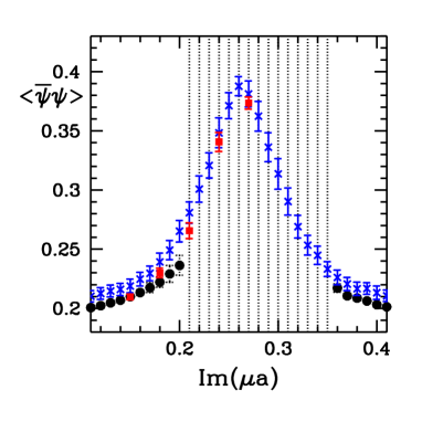
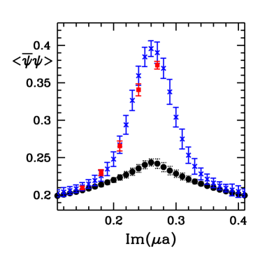
Figure 3: (a) The left panel shows a well functioning error estimate. The squares correspond to direct simulations (out of $60000$ configurations), the crosses denote the results of the multi-parameter reweighting method (out of $\approx 2500$ independent configurations) while the circles are the points of the Glasgow-type reweighting (out of $\approx 7000$ independent configurations). (b) In the right panel the meaning of the symbols are unchanged but the sample sizes for the reweighting techniques are decreased to 1200 independent configurations. Noticeably, in case of the Glasgow-type reweighting the fact that the sample does not contain any configuration from the target phase causes systematic errors in the expectation values and mainly in their uncertainties. This is because in case of strong phase transitions – like in our case – it is far too difficult to define a reliable thermalization stage by virtue of the weights. By increasing the sample size helps in this situation leading to the results of the left panel.

To illustrate the new technique let us take a look at the $n_{f}=4$ flavour case at $m_{q}a=0.05$ bare quark mass on $4\cdot 6^{3}$ size lattice at imaginary chemical potential. Note that for purely imaginary chemical potentials direct simulation is possible, therefore it is possible to check the validity of any possible error estimation method. We carried out simulations at Im$(\mu)=0$ in the phase transition point, i.e. at $\beta=5.04$ ($\approx 2500$ independent configurations) and at $\beta=5.085$ ($\approx 7000$ independent configurations). From these two starting points with the use of the reweighting we tried to predict the plaquette ($Pl$) and the $\bar{\psi}\psi$ expectation values and their uncertainties at $\beta=5.085$ and Im$(\mu)\neq 0$, that is at the target, imaginary chemical potential values. We calculated the plaquette and the $\bar{\psi}\psi$ expectation values by (14) at the target points, and we also used the new Metropolis-type method defined above which leads to very similar results.

The results are shown in Figure 3 (see explanation there). The infinitely large errors of the single-parameter reweighting (Glasgow-method) indicate that the whole sample is thermalization, that is it does not provide information about the expectation value in the required point. In the right panel of Figure 3 the second problem (lack of relevant configuration) mentioned above is seen.

When we determine the EoS the jackknife errors are suitable to estimate the uncertainties of the reweighted quantities in an appropriate region. We used the new error estimates only to provide the limit of the applicability of the reweighting procedure and of the jackknife method.

We can define reweighting lines on the $\beta$–$\mu$ plane so as to make the least possible mistake during the reweighting procedure. To do this we introduce the notion of overlap measure which we denote by $\alpha$. The overlap measure is the normalised number of different configurations in the sample created with the Metropolis-type reweighting after cutting off the thermalization. We plotted the contour lines of $\alpha$ in the left panel of Figure 4. The dotted areas are unattainable, that means here the overlaps vanish, the errors are infinitely large. The best reweighting line can be defined for each simulation point. For a given value of $\mu$ we choose $\beta$ so that $\alpha$ be maximal. The points of the best reweighting lines are given by the rightmost points of the contours of the overlap in Fig. 4 (a).

Then the best reweighting lines are the contours of constant overlap or equivalently of constant error.

     

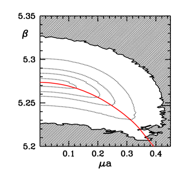
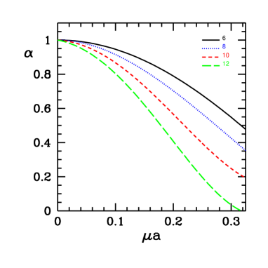
Figure 4: (a) The left panel shows the real chemical potential–$\beta$ plane. 33000 configurations were simulated at the parameter set at the critical $\beta$ in the $n_{f}=2+1$ flavour case. The dotted lines are the contours of the constant overlap. The dotted area is the unknown territory where the overlap vanishes. The solid line is the phase transition line determined by the peaks of susceptibility. (b) In the right panel the volume and the $\mu$ dependence of the overlap ($\alpha$) is shown. Upper curves correspond to smaller lattice sizes, $4\cdot 6^{3}$, $4\cdot 8^{3}$, $4\cdot 10^{3}$ and $4\cdot 12^{3}$ respectively.

The right panel of Figure 4 shows the $\mu$ dependence of the overlap at fixed $\beta$ and quark mass parameters for different volumes ($V=4\cdot 6^{3}$, $4\cdot 8^{3}$, $4\cdot 10^{3}$ and $4\cdot 12^{3}$). As expected, for fixed $\mu$ larger volumes result in worse overlap. One can define the “half-width” ($\mu_{1/2}$) of the $\mu$ dependence by the chemical potential value at which $\alpha=1/2$. One observes an approximate scaling behaviour for the half-width: $\mu_{1/2}\propto V^{-\gamma}$ with $\gamma\approx 1/3$.

It is obvious that the two-parameter reweighting used previously does not follow the LCP ($\beta$ gets smaller but the quark mass remains $m_{0}a$). Nevertheless, the best reweighting line along the LCP can be determined by two techniques. One of them is the three-parameter reweighting, the other one is the interpolating method.

As it can be seen in the left panel of Figure 4, the change in $\beta$ is not very large for the two-parameter reweighting. Therefore, one can remain on the LCP by a simultaneous, small change of the mass parameter of the lattice action. This results in a three-parameter reweighting (reweighting in $ma$, $\beta$ and $\mu a$). Similarly to the two-parameter reweighting one can construct the best three-parameter reweighting line.

Another possibility to stay on the line of constant physics at finite $\mu$ is the interpolating technique. One uses the two-parameter reweighting for two LCP’s and interpolates between them. The result of this method and the predicition of the three-parameter reweighting agree quite well. This indicates that the requirement for the best overlap selects the same weight lines even for rather different methods.

5 Equation of state at non-vanishing chemical potential

In this section we study the EoS at finite chemical potential. Since we are interested in the physics of finite baryon density we use $\mu=\mu_{u}=\mu_{d}\neq 0$ for the two light quarks and $\mu_{s}=0$ for the strange quark.

The pressure ($p$) can be obtained from the partition function as $p$=$T\cdot\partial\log Z/\partial V$ which can be written as $p$=$(T/V)\cdot\log Z$ for large homogeneous systems. On the lattice we can only determine the derivatives of $\log Z$ with respect to the parameters of the action ($\beta,m,\mu$), so $p$ can be written as a contour integral[16]:

$$\frac{p}{T^{4}} = \frac{1}{T^{3}V}\int d(\beta,m,\mu)\left(\left\langle\frac{\partial(\log Z)}{\partial\beta}\right\rangle,\left\langle\frac{\partial(\log Z)}{\partial m}\right\rangle,\left\langle\frac{\partial(\log Z)}{\partial\mu}\right\rangle\right).$$ (16)

The integral is by definition independent of the integration path. The chosen integration paths are shown on Fig 5.

The energy density can be written as $\epsilon=(T^{2}/V)\cdot\partial(\log Z)/\partial{T}+(\mu T/V)\cdot\partial(\log Z)/\partial\mu$. By changing the lattice spacing $T$ and $V$ are simultaneously varied. The special combination $\epsilon-3p$ contains only derivatives with respect to $a$ and $\mu$:

$$\frac{\epsilon-3p}{T^{4}}=-\left.\frac{a}{T^{3}V}\frac{\partial\log(Z)}{\partial a}\right|_{\mu}+\left.\frac{\mu}{T^{3}V}\frac{\partial(\log Z)}{\partial\mu}\right|_{a}.$$ (17)

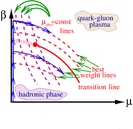
Figure 5: Illustration of the integral method at finite chemical potential (left panel). The solid lines are $\mu={\rm const}$ lines on the $\mu a-\beta$ plane. Dashed lines are the best reweighting lines starting from different simulation points. Arrows show the path of integration we used when evaluating eq. (7.6).

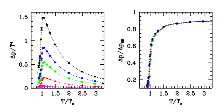
Figure 6: The equation of state at, $\mu_{B}=100$, 210, 330, 410 and 530 MeV. The left panel shows the pressure difference between the $\mu=0$ and $\mu\neq 0$ cases normalized by $T^{4}$, whereas on the right panel the normalization is done by the $N_{t}=4$ lattice Stefan-Boltzman limit. Note, that $\Delta p/\Delta p^{SB}$ seems to show some scaling behaviour (it depends mostly on the temperature; whereas its dependence on $\mu$ is much weaker). Thus, the $\mu$ dependence of $\Delta p$ is almost completely given by the $\mu$ dependence of the free gas.

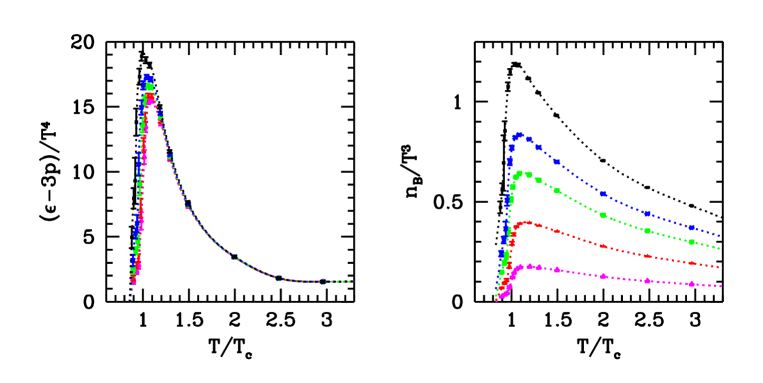
Figure 7: (a) $(\epsilon-3p)/T^{4}$ (b) Dimensionless baryon number density as a function of $T/T_{c}$ at $\mu_{B}$=100,210,330,410 MeV and $\mu_{B}$=530 MeV.

We present lattice results on $\Delta p(\mu,T)=p(\mu\neq 0,T)-p(\mu=0,T)$, $\epsilon(\mu,T)$-3$p(\mu,T)$ and $n_{B}(\mu,T)$. Our statistical errorbars are also shown. They are rather small, in many cases they are even smaller than the thickness of the lines.

On the left panel of Fig. 6 we present $\Delta p/T^{4}$ for five different $\mu$ values. On the right panel normalisation is done by $\Delta p^{SB}$, which is $\Delta p(\mu,T\rightarrow\infty)$. Notice the interesting scaling behaviour. $\Delta p/\Delta p^{SB}$ depends only on T and it is practically independent from $\mu$ in the analysed region. The left panel of Fig. 7 shows $\epsilon$-3$p$ normalised by $T^{4}$, which tends to zero for large $T$. The right panel of Fig. 7 gives the dimensionless baryonic density as a function of $T/T_{c}$ for different $\mu$-s.

The error coming from reweighting has been discussed previously. Another source of error is the finiteness of the physical volume. The volume dependence of physical observables is smaller than the statistical errors for the plaquette average or quark number density.

6 Conclusions, outlook

We studied the thermodynamical properties of QCD at finite chemical potential. We used the overlap improving multi-parameter reweighting method. Our primary goal was to determine the equation of state (EoS) on the line of constant physics (LCP) at finite temperature and chemical potential.

We have pointed out that even at $\mu$=0 the EoS depends on the fact whether we are on an LCP or not. According to our findings pressure and $\epsilon$ - 3p (interacion measure) on the LCP have different high temperature behaviour than in the “non-LCP approach”.

We discussed the reliability of the reweighting technique. We introduced an error estimate, which successfully shows the limits of the method yielding infinite errors in the parameter regions, where reweighting gives wrong results. We showed how to define and determine the best weight lines on the $\mu$–$\beta$ plane.

We discussed the two-parameter reweighting technique. Two techniques were presented (three-parameter reweighting and the interpolating method) to stay on the LCP even when reweighting to non-vanishing chemical potentials.

We calculated the thermodynamic equations for $\mu\neq 0$ and determined the EoS along an LCP. We presented lattice data on the pressure, the interaction-measure and the baryon number density as a function of temperature and chemical potential. The physical range of our analysis extended upto $500-600$ MeV in temperature and baryon chemical potential as well.

Clearly much more work is needed to get the final form of non-perturbative EoS of QCD. Extrapolation to the thermodynamic and continuum limits is a very CPU demanding task in the $\mu\neq 0$ case. Physical $m_{\pi}/m_{\rho}$ ratio should be reached by decreasing the light quark mass. Finally, renormalised LCP’s should be used when evaluating thermodynamic quantites.

References

- [1] F. Wilczek, hep-ph/0003183; M. G. Alford, K. Rajagopal and F. Wilczek, Phys. Lett. B 422 247 (1998); M. G. Alford, K. Rajagopal and F. Wilczek, Nucl. Phys. B 537 443 (1999);
- [2] R. Rapp, T. Schafer, E. V. Shuryak and M. Velkovsky, Phys. Rev. Lett. 81 53 (1998); K. Rajagopal and F. Wilczek, hep-ph/0011333.
- [3] For recent lattice reviews see: J. B. Kogut, Nucl. Phys. Proc. Suppl. 119, 210 (2003); Z. Fodor, Nucl. Phys. A 715, 319 (2003); E. Laermann and O. Philipsen, hep-ph/0303042; S. Muroya, A. Nakamura, C. Nonaka and T. Takaishi, Prog. Theor. Phys. 110, 615 (2003); S. D. Katz, hep-lat/0310051.
- [4] P. Hasenfratz and F. Karsch, Phys. Lett. B 125 308 (1983).
- [5] J. B. Kogut, H. Matsuoka, M. Stone, H. W. Wyld, S. H. Shenker, J. Shigemitsu and D. K. Sinclair, Nucl. Phys. B 225 93 (1983).
- [6] Z. Fodor and S. D. Katz, Phys. Lett. B 534 87 (2002), [arXiv:hep-lat/0104001].
- [7] Z. Fodor and S. D. Katz, JHEP 0203 014 (2002).
- [8] Z. Fodor, S. D. Katz and K. K. Szabo, Phys. Lett. B 568 73 (2003).
- [9] F. Csikor, G. I. Egri, Z. Fodor, S. D. Katz, K. K. Szabo and A. I. Toth, hep-lat/0104016
- [10] C. R. Allton et al., Phys. Rev. D 66 074507 (2002).
- [11] C. R. Allton, S. Ejiri, S. J. Hands, O. Kaczmarek, F. Karsch, E. Laermann, C. Schmidt Phys. Rev. D 68 014507 (2003).
- [12] S. Choe et al., Phys. Rev. D 65 054501 (2002).
- [13] P. de Forcrand and O. Philipsen, Nucl. Phys. B 642 290 (2002).
- [14] P. de Forcrand and O. Philipsen, Nucl. Phys. B 673, 170 (2003).
- [15] M. D’Elia and M. P. Lombardo, Phys. Rev. D 67, 014505 (2003).
- [16] J. Engels, J. Fingberg, F. Karsch, D. Miller and M. Weber, Phys. Lett. B 252 625 (1990).
- [17] C. R. Allton, hep-lat/9610016.
- [18] C. W. Bernard et al. [MILC Collaboration], Phys. Rev. D 55 6861 (1997).
- [19] J. Engels, R. Joswig, F. Karsch, E. Laermann, M. Lutgemeier and B. Petersson, Phys. Lett. B 396 210 (1997).
- [20] F. Karsch, E. Laermann and A. Peikert, Phys. Lett. B 478 447 (2000).
- [21] S. Ejiri, arXiv:hep-lat/0401012.
- [22] A. M. Ferrenberg and R. H. Swendsen, Phys. Rev. Lett. 61 2635 (1988).
- [23] A. M. Ferrenberg and R. H. Swendsen, Phys. Rev. Lett. 63 1195 (1989).
- [24] I. M. Barbour, S. E. Morrison, E. G. Klepfish, J. B. Kogut and M. P. Lombardo, Nucl. Phys. Proc. Suppl. 60A 220 (1998).
- [25] F. Csikor, Z. Fodor and J. Heitger, Phys. Rev. Lett. 82 21 (1999).
- [26] Y. Aoki, F. Csikor, Z. Fodor and A. Ukawa, Phys. Rev. D 60 013001 (1999).
- [27] Ferrenberg, Landau, Swendsen Phys. Rev. E 51 5092(1995).
- [28] M. E. J. Newman, R. G. Palmer J. Stat. Phys. 97 1011 (1999).