Lattice QCD at finite density

Abstract

QCD at finite density presents specific challenges to lattice gauge theory. Nonetheless, a region of the QCD phase diagram up to moderately large baryon chemical potentials has been successfully explored on the lattice and new results and idea are continuously emerging.

I will outline the lattice formulation of QCD, introduce the calculational schemes currently used to treat a nonzero baryon density, and mention lattice methods alternative to MonteCarlo, including the strong coupling expansion which might give access to the the superconducting phase of QCD. The results for the critical line, and the different phases will be discussed highlighting the strength of the different methods, as well as the possible comparisons with phenomenological models.

1 Introduction

Lattice discretization combined with importance sampling affords the possibility of doing first principles calculations of the properties of strongly interacting matter [1]. Questions to be addressed obviously include the study of QCD with physical values of the quark masses, and in the thermodynamic region within the range of current, and planned, experiments at BNL and CERN.

While addressing these phenomenological points, one is lent to consider more theoretical questions – patterns of chiral symmetry, mechanisms of confinement, topological structures, gauge field dynamics…– on general grounds. To this end, it is not only legitimate, but also useful (and sometimes mandatory), to consider QCD in a larger parameter space. This can be achieved in a numerical simulation, where not only we can tune experimental parameters such as baryon chemical potential, temperature, isospin chemical potential, but we can also play with the number of colors and flavors, the value of the bare masses, the gauge coupling, or we can make imaginary some external fields. In the following QCD will thus be a generic name for any of these variants – to be specified whenever needed – of the “real world” theory of strong interactions.

In this note we will be mostly concerned with the phases of QCD at finite baryon density. Let me then mention, as a last introductory remark, that there are strong differences between physical mechanisms of phase transitions in QCD at high baryon density and high temperature. At high temperature the chiral transition is a transition from an ordered to a disordered state, characterized by light baryons; deconfinement is associated with string breaking due to recombination with light pairs; topological structures include instanton molecules. At high baryon density instabilities at the Fermi surface induce unusual patterns of chiral symmetry such as color superconductivity or superfluidity; string breaking might be further enhanced by recombination with real particles; topological structures are mostly likely instanton chains. These differences between high temperature and high density might provide further insight into chiral symmetries, gluon dynamics and topological structures, and further motivate the study of a nonzero baryon density on a lattice.

2 Formulation

Let us remind ourselves how to introduce a chemical potential $\mu$ for a conserved charge $\hat{N}$ in the density matrix $\hat{\rho}$ in the Grand Canonical formalism, which is the one appropriate for a relativistic field theory [1]:

$$\hat{\rho} = e^{-(H-\mu\hat{N})/T}$$ (1)

$$\cal Z(T,\mu) = Tr\hat{\rho}=\int d\phi d\psi e^{-S(\phi,\psi)}$$ (2)

The path integral representation of the grand partition function $\cal Z$ in the Euclidean space gives the temperature as the reciprocal of the imaginary time:

$$S(\phi,\psi)=\int_{0}^{1/T}dt\int d^{d}x{\cal L}(\phi,\psi)$$ (3)

with periodic boundary conditions in time for bosons $\phi(t=0,\vec{x})=\phi(t=1/T,\vec{x})$ and antiperiodic for fermions $\psi(t=0,\vec{x})=-\psi(t=1/T,\vec{x})$.

All in all, ${\cal Z}$ at finite temperature $T$ and density $\mu$ is the partition function of a statistical system in d+1 dimension, where $T$ is the reciprocal of the imaginary time, and $\mu$ couples to any conserved charge. This representation, which is the starting point for a lattice calculation, allows us to deal with thermodynamics and spectrum exactly on the same footing.

The theory is regularised on a space time lattice: a regular four dimensional grid with $N_{s}$ points in each space directions, $N_{t}$ points in the imaginary time direction, and spacing $a$. We refer to the very many excellent reviews and textbooks for background material on lattice field theory, and we briefly summarize here the specific aspects of lattice QCD thermodynamics which will be useful in the following.

The temperature $T$ on a lattice is the same as in the continuum: $T=1/N_{t}a$, $N_{t}a$ being the lattice extent in the imaginary time direction (while, ideally, the lattice spatial size should be infinite). A lattice realisation of a finite density of baryons, instead, poses specific problems: the naive discretization of the continuum expression $\mu\bar{\psi}\gamma_{0}\psi$ would give an energy $\epsilon\propto\frac{\mu^{2}}{a^{2}}$ diverging in the continuum (${a\to 0}$) limit [2].

The problem could be cured by introducing appropriate counterterms, however the analogy between $\mu$ and an external field in the $0_{th}$ (temporal) direction offers a nicer solution by considering the appropriate lattice conserved current [2]. This amounts to the following modification of the fermionic part of the Lagrangian for the $0_{th}$direction $L_{F}^{0}$:

$$L_{F}^{0}(\mu)=\bar{\psi}_{x}\gamma_{0}e^{\mu a}\psi_{x+\hat{0}}-\bar{\psi}_{x+\hat{0}}\gamma_{0}e^{-\mu a}\psi_{x}$$ (4)

while the remaining part of the Lagrangian is unchanged. This yields the current:

$$J_{0}=-\partial_{\mu}L=-\partial_{\mu}{L_{F}}^{0}(\mu)=\bar{\psi}_{x}\gamma_{0}e^{\mu a}\psi_{x+\hat{0}}+\bar{\psi}_{x+\hat{0}}\gamma_{0}e^{-\mu a}\psi_{x}$$ (5)

This representation of $J_{0}$ is amenable to a simple interpretation: the time forward propagation is enhanced by $e^{\mu a}$, while the time backward propagation is discouraged by $e^{-\mu a}$; hence, the link formulation generates a particles–antiparticles asymmetry. In addition, note that $\int J_{0}=N-\bar{N}$ as it should. An alternative way to look at the link formulation introduces an explicit dependence on the fugacity $e^{\mu/T}$ via an unitary transformation for the fields [3]. In this way $L(\mu)=L(0)$, and the $\mu$ dependence is on the boundaries, via the fugacity $e^{\mu/T}$: $\psi(x+N_{T})=-e^{\mu aN_{T}}\psi(x)=-e^{\mu/T}\psi(x)$. This is analogous to the continuum case[4].

3 Calculational Schemes

Having set up the formalism, the task is to compute

$${\cal Z}=\int dUd\psi e^{-S(U,\psi)}$$ (6)

where from now on the Lagrangian defining the Action will be that of lattice QCD, containing gluon fields $U$ and quark fields $\psi$.

We have two options. We might integrate out gluons first:

$$\int dUd\psi d\bar{\psi}{\cal Z}(T,\mu,\bar{\psi},\psi,U)\simeq\int d\psi d\bar{\psi}{\cal Z}(T,\mu,\bar{\psi},\psi)$$ (7)

This produce an effective approximate fermion model: the procedure is physically appealing, but not systematically improvable, but for one special (lattice) case (see below). Alternatively, we might integrate out fermions exactly, by taking advantage of the bilinearity of the fermionic part of the Lagrangian $L=L_{YM}+L_{F}=L_{YM}+\bar{\psi}M(U)\psi$ :

$$\int dUd\psi d\bar{\psi}{\cal Z}(T,\mu,\bar{\psi},\psi,U)=\int dUe^{-(S_{YM}(U)-log(detM))}$$ (8)

The “effective” model we build this way is exact: the price to pay being that its physical interpretation is not as clear as for effective fermion models. Anyway, this expression is the starting point for numerical calculations: the fact that in many cases they are highly successful tell us that the configuration space is well behaved enough that only a minor subset of configurations, although carefully chosen via importance sampling, suffice to produce reasonable results.

3.1 Effective Fermionic Models: analytical approaches

Let us start by following the first idea, namely integrating out the gluon fields so to define an effective fermionic Action. This is a time honored approach, leading, for instance, to the instanton model Hamiltonian, hence to the exciting discoveries on the QCD phase diagram of the last five years[5] .

On the lattice, one very interesting approach leading to a fermionic model is provided by the strong coupling expansion: in the infinite gauge coupling limit the Yang Mills term decouples from the Action, and the integral over the gauge fields can be carried out exactly.

The starting point is the QCD lattice Lagrangian:

$$S = -1/2\sum_{x}\sum_{j=1}^{3}\eta_{j}(x)[\bar{\chi}(x)U_{j}(x)\chi(x+j)-\bar{\chi}(x+j)U^{\dagger}_{j}(x)\chi(x)]$$

$$-1/2\sum_{x}\eta_{0}(x)[\bar{\chi}(x)U_{0}(x)\chi(x+0)-\bar{\chi}(x+0)U^{\dagger}_{0}(x)\chi(x)]$$

$$-1/3\sum_{x}6/g^{2}\sum_{\mu,\nu=1}^{4}[1-reTrU_{\mu\nu}(x)]$$

$$+\sum_{x}m\bar{\chi}\chi$$

The $\chi,\bar{\chi}$ are the staggered fermion fields living on the lattice sites, the $U$’s are the $SU(N_{c})$ gauge connections on the links, the $\eta$’s are the lattice Kogut–Susskind counterparts of the Dirac matrices, and the chemical potential is introduced via the time link terms $e^{\mu}$, $e^{-\mu}$ as discussed above. This time we have written down explicitly the lattice Action to show that the pure gauge term
$S_{G}=-1/3\sum_{x}6/g^{2}\sum_{\mu,\nu=1^{4}}[1-reTrU_{\mu\nu}(x)]$ contains the gauge coupling in the denominator, hence it disappears in the infinite coupling limit. Consequently, one can perform independent spatial link integrations, leading to

$${\cal Z}=\int\prod_{timelinks}dU_{t}d\bar{\chi}d\chi e^{-1/{4N}\sum_{<x,y>}\bar{\chi}(x)\chi(x)\bar{\chi}(y)\chi(y)}e^{-S_{t}}$$ (10)

where $\sum_{<x,y>}$ means sum over nearest neighboring links, terms of higher order have been dropped, and we recognize a four fermion interaction [6]. Further manipulations yield the mean field effective potential:

$$V_{eff}(<\bar{\psi}\psi>,{\mu})=2{cosh(rN_{t}N_{c}\mu)}+sinh[(N_{t}+1)N_{c}<\bar{\psi}\psi>]/sinh(N_{t}<\bar{\psi}\psi>)$$

which we quote for further reference. A standard analysis of $V_{eff}$ finally gives the condensate as a function of temperature and density, and allows the reconstruction of the phase diagram.

More recently this approach has been furthered both in two [8] and three colors[9], and new developments on cluster algorithms have appeared as well [10].

In order to describe in detail the rich physics of the finite density phase, one needs both to include higher order terms into the strong coupling expansion, as well as to go beyond a simple mean field analysis, which assumes an homogeneous background. The question is as to whether such improved strong coupling approaches would be able to generate a four fermion term with the correct flavor structure as well as order of magnitude, thus opening the possibility of a systematically improvable approach to finite density QCD, including the study of the superconducting phase.

3.2 Effective Gluonic Models: Importance Sampling and the positivity issue

Let us write again

$${\cal Z}(T,\mu)=\int dUe^{-(S_{YM}(U)-log(\det M))}$$ (11)

When $\det M>0$ the functional integral can be evaluated with statistical methods, sampling the configurations according to their importance $(S_{YM}(U)-log(\det M))$. For this to be possible the would-be-measure ($\det M$) has to be positive.

Let me mention at this point that the factorization method [7] might alleviate the problems of complex measures by guiding the simulations along a sensible path in the phase space. I will not dwell on this interesting development which is not really in the scope of an introductory review, but I wish to call on it the attention of the interested reader, as it really seems to offer some promise, and has been already tested in random matrix models.

In QCD with an even number of flavors, and zero chemical potential, standard importance sampling simulations are possible if $\det M$ is real, which is true if $M^{\dagger}=-PMP^{-1}$ where $P$ is any non singular matrix. In the most popular lattice fermion formulation this holds: for Wilson fermions $P=\gamma_{5}$ and for staggered fermions $P=I$ (note that this basically expresses a particle–antiparticle symmetry). We will consider staggered fermions from now on.

Consider now the relationship $M^{\dagger}(\mu_{B})=-M(-\mu_{B})$ implying that reality is lost when ${\rm Re}\mu\neq 0$: the reality of the determinant is lost, and with it the possibility of doing simulations with non zero chemical potential, when we want to create a particle antiparticle asymmetry. On the other hand a purely imaginary chemical potential does not spoil the reality of the determinant: indeed, even if an imaginary chemical potential can be used to extract information at real chemical potential, it does not create any real particle–antiparticle asymmetry and it is natural that the fermion determinant remains real.

Note that in QCD with two color the determinant remains positive with nonzero real chemical potential: indeed, in that case quarks and antiquarks transform under equivalent representation of the color group and are, essentially, the same particle. Other important models with a real determinant include finite density of isospin [12] and four fermion models [11]. These aspects will be reviewed by Don Sinclair at this meeting [12], so I shall not further discuss them.

All in all, if we want to extract information useful for QCD at nonzero baryon density by use of standard MonteCarlo sampling we will have to use information from the accessible region:

$${\rm Re~{}~{}}\mu=0,{\rm Im~{}~{}}\mu\leq 0$$

4 Overview of the methods

To begin with, it is useful to think of the theory in the $T,\mu^{2}$ plane. Let us then discuss the phase diagram from the perspective of analyticity and positivity of the partition function and of the determinant. One important consideration to keep in mind: the Gran Canonical partition function has to be positive. It is only the determinant which can change sign, or even be complex, on single configurations.

Let us consider a mapping from complex $\mu$ to complex $\mu^{2}$. Because of the symmetry properties of the theory, this mapping can be done without loss of generality. Let us note then that ${\cal Z}(\mu^{2})$ is real valued for real $\mu^{2}$: this is a situation familiar from condensed matter: the partition function is real where the external parameter is real, complex otherwise.

The reality region for the partition function represents states which are physically accessible. The reality region for the determinant represents the region which is amenable to an importance sampling calculation: ${\rm Re}\mu^{2}\leq 0$. The methods which have been applied so far are

• $\mu=0$ Derivatives, Reweighting, Expanded reweighting

• $\mu^{2}\leq 0$ Imaginary chemical potential

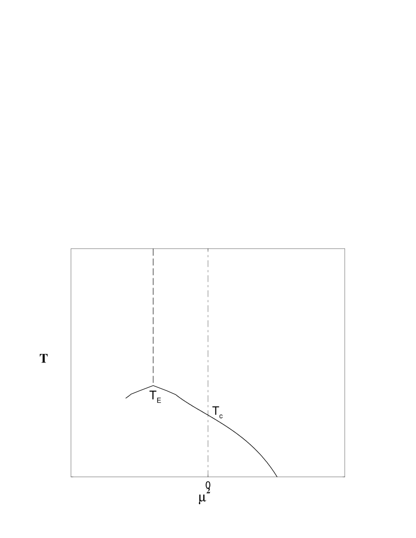
Figure 1: Sketch of the phase diagram in the $\mu^{2},T$ plane: the solid line is the chiral transition, the dashed line is the Roberge Weiss transition. Simulations can be carried out at $\mu^{2}\leq 0$ and results continued to the physical domain $\mu^{2}\geq 0$. The derivative and reweighting methods have been used so far to extract informations from simulations performed at $\mu=0.$ The imaginary chemical potential approaches uses results on the left hand half plane. Different methods could be combined to improve the overall performance.

4.1 Derivatives at $\mu=0.0$

This is one early attempt at exploring the physics of nonzero quark density: the derivatives can be formally computed at $\mu=0$ [13]. The obvious limitation is that we do not really know how far from the $\mu=0$ axis can we get. Nonetheless, such derivatives are interesting per se, and the region where derivatives are clearly different from zero is the natural candidate for the application of other methods.

4.2 Reweighting from $\mu=0$

Back in the 80’s Ian Barbour and collaborators proposed to calculate ${\cal Z}(\mu)$ from simulations at $\mu=0$:

$${\cal Z}=\left<{{|M(\mu)|}\over{|M(\mu=0)|}}\right>_{\mu=0}$$ (12)

In other words, the chemical potential $\mu$ of the target ensemble at that of the simulation ensemble – $\mu=0$ – are different: the properties of the target ensemble can be inferred from those of the simulation ensemble, provided that there is a sizable overlap between the two [14].

At $T=0$ the Glasgow procedure fails because of a poor overlap (aside, the strong coupling calculations were quite useful to asses these problems), and it is instructive to study the overlap problem as seen in the Gross Neveu model, where there is no sign problem [11], and the results obtained with reweighting methods can be compared with those of exact simulations [15].

The distribution of the order parameter (the $\sigma$ particle) helps visualizing the problem (see Fig. 2): the order parameter distributions in the two phases do not overlap[11].

Figure 2: The overlap problem in the Gross Neveu model[15]: the exact distributions of the $<\sigma>$ fields in the broken (left) and symmetric (right) phase are non–overlapping.

It is interesting to note that there are indeed examples of successful reweighting at $\mu\neq 0$. Let us consider 1-dim $SU(3)$ which can be exactly solved at nonzero baryon density[16] and can thus serve as a test bed for experiments. The distribution of the partition function zeros was computed and found to reproduce the correct results one the statistics were sufficiently high[22].

Figure 3: Successful reweighting in one dimensional QCD[22]: exact Z’s zeros in the complex $\mu$ plane (diamonds) and the cloud of zeros obtained from reweighting with a very poor statistics(leftt). On the rigth the zeros from an high statistics reweighting simulation reproducing the exact result.

The conclusion from these early studies was that reweighting fails in QCD at zero temperature because of a poor overlap, and that the reason behind the failure is practical rather than conceptual: the situation can be ameliorated if a better starting point were used.

4.3 Fodor and Katz’s multiparameter reweighting

The prescription for ameliorating the overlap is due to Fodor and Katz [17][18] whose Multiparameter reweighting use fluctuations around $T_{c}$ at $\mu=0$ to explore the critical region. Making reference to Fig. 2, and oversimplifying: instead of trying to reweight the distribution at zero temperature in the broken phase, which is obviously hopeless, one might hope that a distribution generated at zero density, and close to the critical temperature, bears more resemblance with the target distribution along the critical line, and is thus amenable to a successful reweighting.

The strategy was applied to QCD [17][18] . The improvement obtained is impressive and produced the first quantitative results for the critical line at nonzero chemical potential in QCD: we will come back to this in the section on results. A multistep reweighting proposed by Crompton [19] might well produce a further improvement.

4.4 Taylor Expanded Reweighting

The Bielefeld-Swansea collaboration suggested a Taylor expansion of the reweighting factor as a power series in $\lambda=\mu/T$, and similarly for any operator[21] [20] .

This strategy is computationally very convenient as it greatly simplifies the calculation of the determinant. Expectation values are then given by

$$\langle{\cal O}\rangle_{(\beta,\mu)}={{\langle({\cal O}_{0}+{\cal O}_{1}\lambda+{\cal O}_{2}\lambda^{2}+\ldots)\exp({\cal R}_{1}\lambda+{\cal R}_{2}\lambda^{2}+\ldots-\Delta S_{g})\rangle_{\lambda=0,\beta_{0}}}\over{\langle\exp({\cal R}_{1}\lambda+{\cal R}_{2}\lambda^{2}+\ldots-\Delta S_{g})\rangle_{\lambda=0,\beta_{0}}}}.$$ (13)

Results - to be discussed later- have been obtained both for the critical line and thermodynamics.

4.5 Imaginary Baryon Chemical Potential

This method uses information from all of the negative $\mu^{2}$ half plane (Fig. 1) to explore the positive, physical relevant region. An imaginary chemical potential $\nu$ in a sense bridges Canonical and Grand Canonical ensemble[23]:

$${\cal Z_{C}(N)}=\frac{\beta}{2\pi}\int_{0}^{2\pi/\beta}d\nu{\cal Z_{GC}}(i\nu)e^{-i\beta\nu N}$$ (14)

The main physical idea behind any practical application is that at $\mu=0$ fluctuations allow the exploration of $N_{b}\neq 0$ hence tell us about $\mu\neq 0$. Mutatis mutandis, this is the same condition for the reweighting methods to be effective: the physics of the simulation ensemble has to overlap with that of the target ensemble.

A practical way to use the results obtained at negative $\mu^{2}$ relies on their analytical continuation in the real plane. For this to be effective[22] ${\cal Z}(\mu,T)$ must be analytical, nontrivial, and fulfilling this rule of thumb:

$$\chi(T,\mu)=\partial\rho(\mu,T)/\partial\mu=\partial^{2}logZ(\mu,T)/\partial\mu^{2}>0$$ (15)

This approach has been tested in the strong coupling limit [22] of QCD, in the dimensionally reduced model of high temperature QCD [24] and, more recently, in the two color model [25].

Results (to be discussed later) have been obtained for two [26], four [27] and three [28] staggered flavors.

5 Results

The methods just outlined above are workarounds, not real solutions: they are practical tools to circumvent a problem, and, as such, it it not surprising that they have to be applied with a grain of salt, and that their performance depends on the thermodynamic region which is being explored.

In this section I will go through the main issues which have been addressed so far: the critical line, the hadronic phase, the “Roberge Weiss” regime, the quark gluon plasma phase, highlighting the main strengths of the various methods alongside with the results.

5.1 The Critical Line

The critical line has been obtained either by Fodor and Katz [17][18] and by the Bielefeld Swansea collaboration within the multiparameter reweighting or the expanded reweighting approach, which gives $Z(\mu)$ from $Z(0)$. The location of the end point follows naturally within this framework, and its first determination was given in [18] .

De Forcrand and Philipsen have also noticed that the analytic continuation of the critical line from an imaginary $\mu$ is possible [26], and have indicated and applied a strategy for the location of the end point [28].

Also for the calculation of the critical line the consideration of the $T,\mu^{2}$ plane helps the analysis [27]. Model analysis suggests the following parametrization, confirmed by numerical results:

$$(T+aT_{c})(T-T_{c})+k\mu^{2}=0,\;\;\;\;k>0$$ (16)

It encodes reality for real $\mu^{2}$, contains the physical scale $T_{c}$ , is dimensionally consistent, gives $T(\mu=0)=T_{c}$, $T(\mu\neq 0)<T_{c}$ . For instance, the second order approximation $T(T-T_{c})+\mu^{2}/(8ln2)=0$ to the Gross Neveu Model critical line: $1-\mu/\Sigma_{0}=2T/\Sigma_{0}ln(1+e^{-\mu/T})$ is good up to $\mu\simeq T_{c}$, and from the plot in Fig. 4 can see that a second order approximation is good up to $\mu\simeq T_{c}$

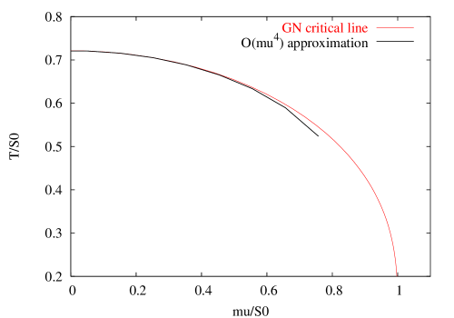
Figure 4: The critical line of the 3d Gross Neveu Model and its polynomial approximation.

Studies of the critical line have indeed found that a simple polynomial approximation suffices to describe the data, within the current precision. Progress on the precision is demonstrated in Fig. 5 [28] where the new results on the three flavor model [28] are superimposed to the older ones with two[26] and four flavors[27].

A crucial issue remains the determination of the endpoint, for which the first estimate was given within the reweithgting method $T_{E}=160\pm 3.5MeV$, $\mu_{E}=725\pm 35MeV$ [18]. Results with improved precisions show a dependence on the mass values. This makes mandatory an extrapolation to physical values of the quark masses, which , in turn, implies a good control on the continuum limit.

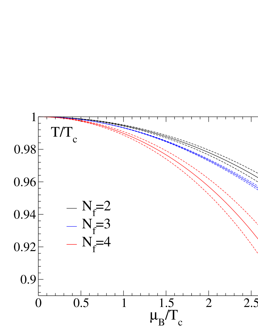
Figure 5: Summary plot[28] for the critical line for $N_{f}=2$[26], $N_{f}=3$ [28], $N_{f}=4$ [27] from imaginary chemical potential calculations.

5.2 Hadronic Phase $T<T_{c}$ I: the hadron resonance gas model

In this region observables are a continuous and periodic function of $\mu_{I}/T$ , analytic continuation in the $\mu^{2}>0$ half plane is always possible, but interesting only when $\chi_{q}(\mu=0,T)>0$.

Taylor expansion and Fourier decomposition are natural parametrization for the observables[27]. In particular, the analysis of the phase diagram in the temperature-imaginary chemical potential plane suggests to use Fourier analysis for $T\leq T_{c}$, as observables are periodic and continuous there. Note that in the infinite strong coupling all of the Fourier coefficients but the first ones will be zero (cfr eq. 3.1).

As the chiral condensate is an even function of the chemical potential, its Fourier decomposition reads:

$$\langle\bar{\psi}\psi\rangle=\sum_{n}a_{F}^{n}\cos(nN_{t}N_{c}\mu_{I})$$ (17)

which is easily continued to real chemical potential.

One cosine fit is actually enough to describe the data up to $T\simeq T_{c}$ in the four flavor model [27]: adding a term $\cos(2N_{t}N_{c}\mu)$ in the expansion does not modify the value of the first coefficients and does not particularly improve the $\chi^{2}$.

This phase was also studied within the reweighting approach[29]. It was confirmed that one single hyperbolic cosine is an excellent approximation to the data, and the result has been interpreted within the framework of the hadron resonance gas model, whose partition function has the single hyperbolic cosine form as the one given by the strong coupling expansions eq. 3.1.

5.3 The Hadronic Phase II: The order of the phase transition, and related endpoints

The analytic continuation of an observable $O$ is valid till $\mu<\mu_{c}(T)$, where the critical value $\mu_{c}(T)$ has to be measured independently. The value of the analytic continuation $O(\mu_{c})$ of an observable $O$ at $\mu_{c}$ defines the discontinuity at the critical point. In turns, this allows the identification of the order of the phase transition. One might wonder which is the meaning of the analytic continuation for $\mu>\mu_{c}(T)$, the one which we have to chop by hand.

It is natural to interpret such analytic continuation as the metastable branch of the observable we are considering, for instance $<\bar{\psi}\psi>$ : it follows the secondary minimum of the associate Landau Ginsburg potential and determines the spinodal point $\mu^{*}$ according to $<\bar{\psi}\psi>=A(\mu-\mu^{*})^{\beta}$. The discontinuity $<\bar{\psi}\psi>(\mu_{c})$ is related to $(\mu_{c}-\mu^{*})$, and both shrinks to zero at the endpoint of a first order transition.

The analytic continuation of the results in the hadronic phase, when cross examined with the results for the critical line, offers an alternative way to study the order of the phase transition: the transition will be second order is the zero of the analytic continuation matches the critical point, first order otherwise. The endpoint of a first order transition can be detected by monitoring $(\mu-\mu^{*})$ as a function of temperature.

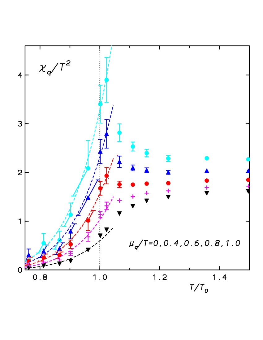
Figure 6: The Bielefeld-Swansea collaboration data contrasted with the hadron resonance gas model [29].

Clearly this approach is specific to the imaginary chemical potential calculations, and give results which should be cross checked with others. For the time being it was confirmed [27] that the transition in the four flavor model remains of first order at nonzero density.

5.4 The Roberge Weiss Regime: $T_{C}<T<T_{E}$

Let us consider region which is comprised between the deconfinement transition, and the endpoint of the Roberge Weiss transition: the analytic continuation is valid till $\mu=\infty$ but the interval accessible to the simulations for $\mu^{2}<0$ is small, as simulations in this area hits the chiral critical line.

The bright side of this is that the nature of the critical line can then be studied without need for an analytic continuation. In Fig. 3 we show the clear correlation between the Polyakov Loop and the chiral condensate at $\mu=0.15$[27][33].

The correlation between chiral and deconfining transition persists at nonzero imaginary chemical potential, see Fig.  7 [27][33]. Obviously, these observations can be immediately continued to real chemical potential : if the difference between the value of the critical $\mu$’s for confinement and chiral symmetry is zero in a finite interval within the analyticity domain (in our case, for $\mu^{2}\leq 0$), it will be zero everywhere within the same domain.

It is also of interest to note that the non–applicability of perturbation theory in this region is almost a theorem: indeed the analytic continuation of the polynomial predicted by perturbation theory for positive $\mu^{2}$ would never reproduce the correct critical behavior at the second order phase transition for $\mu^{2}<0$ , and it is then ruled out.

5.5 The QGP phase : $T_{E}<T$

At high temperature, in the weak coupling regime, perturbation theory might serve as a guidance, suggesting that the first few terms of the Taylor expansion might be adequate in a wider range of chemical potentials. This confirms that the Roberge Weiss critical line has to be strongly first order at high temperature.

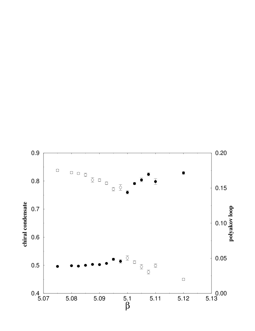
Figure 7: Correlation between $<\bar{\psi}\psi>$ and Polyakov loop at $\mu_{I}=0.15$ [33]. The observed correlation of chiral and deconfining transition must persist at nonzero baryon density[27].

Several analytic models have been proposed to describe the properties of this phase. As one example, we show how a QGP liquid model prediction developed by Letessier and Rafelsky [31]:

$$\Delta P/T^{4}=2(1-2\alpha_{s}/\pi)((\mu/T)^{2})$$ (18)

where $\alpha_{s}=\alpha_{s}(2\sqrt{(\pi T)^{2}+\mu_{q}^{2}})$, compares favorably with reweighting data by Z.Fodor, S.Katz and K.K.Szabo [30]. Very similar conclusions were reached by analyzing quasi-particle models [32].

As a further practical tool for the analysis of this phase, it was proposed [33] to define an “effective prefactor plot” $\Delta PK_{L(N_{t}=4)}/(T^{4}2(\mu/T)^{2})$ which should equal, for instance $2(1-2\alpha_{s}/\pi)$ in the model discussed above, and, in general, which would serve to assess by eye the $\mu$ dependence, if any, of the prefactor of the quadratic term.

It was found that the results approach the perturbative limit at large chemical potential, but corrections at small chemical potential are clearly visible, and become much less severe while approaching the large $\mu$ limit. It would be interesting to understand the connection between these numerical observations and the theoretical work on effective positivity on dense matter[34].

6 Summary/Outlook

QCD at nonzero baryon density is now an active field of research with results emerging from different methods.

The critical line for two, three, two plus one, and four flavors has been computed by various methods, with a substantial agreement. The critical line is well described by a polynomial, and this result can be interpreted in terms of simple models.

The endpoint has been located by different methods, and its determination is currently being sharpened. In the four flavor model, when the transition is of first order, the chiral and deconfining transition remain correlated at nonzero chemical potential.

The analytic continuation from an imaginary chemical potential gives access to the often evasive physics of the metastable branch. It might afford an alternative way to locate the end point and tricritical point.

Three different regimes have been considered and discussed: the hadronic phase results are consistent with the hadron resonance gas model, both from reweighting calculations and imaginary chemical potential approach; the Roberge Weiss regime is eminently nonperturbative, and in this regime we have the possibility to study the nature of the chiral transition at nonzero chemical potential without performing any analytic continuation; the Quark Gluon Plasma phase seems well described by simple models, but corrections are visible and still need being quantified.

Assessing the validity of simple models at high temperature/density, besides being extremely interesting per se, would also open the possibility of doing non equilibrium calculations based on these models. The imaginary chemical potential approach seems to be particularly well suited for this task.

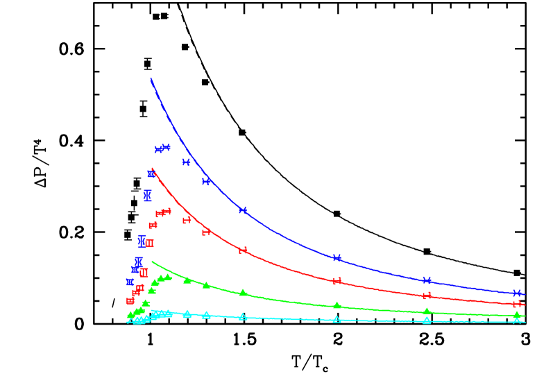
Figure 8: Lattice results by Fodor, Katz and Szabo contrasted with a Quark Gluon Plasma liquid model [31].

The three methods we have discussed are mature for quantitative studies in realistic cases. A nice possibility is offered by a combination of these methods: for instance either reweighting or direct calculations of derivatives could be performed at nonzero $\mu$ to improve the accuracy of the results at negative $\mu^{2}$, and of the ensuing analytic continuation to real $\mu$.

Finally, it might well be that other methods such as $\chi QCD$ which in the past encountered difficulties at zero temperature and nonzero baryon density will prove successful in the richer high temperature regime [12].

References

- [1] For introductory material, and recent reviews, see e.g. S. Muroya, A. Nakamura, C. Nonaka and T. Takaishi, Prog. Theor. Phys. 110, 615 (2003); E. Laermann and O. Philipsen, Status of lattice QCD at finite temperature arXiv:hep-ph/0303042.; F. Karsch and E. Laermann, Thermodynamics and in-medium hadron properties from lattice QCD arXiv:hep-lat/0305025 ; S. D. Katz, Lattice QCD at finite T and arXiv:hep-lat/0310051.
- [2] J. B. Kogut, H. Matsuoka, M. Stone, H. W. Wyld, S. H. Shenker, J. Shigemitsu and D. K. Sinclair, Nucl. Phys. B 225, 93 (1983); P. Hasenfratz and F. Karsch, Phys. Lett. B 125, 308 (1983).
- [3] P. E. Gibbs, Phys. Lett. B172, 53(1986); J. C. Vink, Nucl. Phys. B 323, 399 (1989).
- [4] see T. S. Evans, The Condensed Matter Limit of Relativistic QFT , in ’Dalian Thermal Field’ (1985) p. 283, arXiv:hep-ph/9510298 for a particularly clear discussion of this point and its implications.
- [5] M. G. Alford, Ann. Rev. Nucl. Part. Sci. 51, 131 (2001); K. Rajagopal and F. Wilczek, The Condensed Matter Physics of QCD, to appear in ’At the Frontier of Particle Physics / Handbook of QCD’, M. Shifman, ed., (World Scientific), arXiv:hep-ph/0011333; R. Rapp, T. Schafer, E.V. Shuryak, M. Velkovsky , Annals Phys. 280 (2000)35.
- [6] P. Damgaard, Phys.Lett. B143, 210 (1984); van den Doel, Z.Phys. C 29, 79 (1985) , F. Ilgenfritz et al., Nucl.Phys. B 377, 651 (1992); N. Bilic, D. Demeterfi and B. Petersson, Phys.Rev. D 37, 3691 (1988); for work in the Hamiltonian formalism see e.g. E. B. Gregory, S.-H. Guo, H. Kroger, X.-Q. Luo Phys. Rev. D 62 054508 (2000); Y. Umino, Phys.Lett.B492, 385(2000).
- [7] K. N. Anagnostopoulos and J. Nishimura, Phys. Rev. D 66, 106008 (2002); J. Ambjorn, K. N. Anagnostopoulos, J. Nishimura and J. J. M. Verbaarschot, JHEP 0210, 062 (2002); V. Azcoiti, G. Di Carlo, A. Galante and V. Laliena, Phys. Rev. Lett. 89, 141601 (2002);
- [8] Y. Nishida, K. Fukushima and T. Hatsuda, Thermodynamics of strong coupling 2-color QCD with chiral and diquark condensates, arXiv:hep-ph/0306066.
- [9] B. Bringoltz and B. Svetitsky, Nucl. Phys. Proc. Suppl. 119, 565 (2003); B. Bringoltz, Order from disorder in lattice QCD at high density arXiv:hep-lat/0308018.
- [10] S. Chandrasekharan and U. J. Wiese, Phys. Rev. Lett. 83, 3116 (1999).
- [11] S. Hands, S. Kim and J. B. Kogut, Nucl. Phys. B 442, 364 (1995); for recent developments see e.g. S. Hands, J. B. Kogut, C. G. Strouthos and T. N. Tran, Phys. Rev. D 68, 016005 (2003).
- [12] D. K. Sinclair, J. B. Kogut and D. Toublan, Finite density lattice gauge theories with positive fermion determinants arXiv:hep-lat/0311019.
- [13] C. Bernard et al. [MILC Collaboration], Nucl. Phys. Proc. Suppl. 119, 523 (2003); Physical Review D 38, (1988) 2888; Phys. Rev. Lett 59 (1987) 2247; R.V. Gavai and S. Gupta, Phys. Rev. D 64 (2001) 074506; Phys. Rev. D 65 (2002) 094515; R.V. Gavai, S. Gupta and P. Majumbdar, Phys. Rev. D 65 (2002) 054506; Choe et al, Physical Review D 65 (2002) 054501.
- [14] I. M. Barbour, Nucl. Phys. Proc. Suppl. 26, 22 (1992); I. M. Barbour, S. E. Morrison, E. G. Klepfish, J. B. Kogut and M. P. Lombardo, Nucl. Phys. Proc. Suppl. 60A, 220 (1998),
- [15] I. Barbour, S. Hands, J. B. Kogut, M. P. Lombardo and S. Morrison, Nucl. Phys. B 557, 327 (1999).
- [16] N. Bilic and K. Demeterfi, Phys. Lett. B 212, 83 (1988).
- [17] Z. Fodor and S. D. Katz, Phys. Lett. B 534, 87 (2002).
- [18] Z. Fodor and S. D. Katz, JHEP 0203, 014 (2002).
- [19] P. R. Crompton, Nucl. Phys. B 619, 499 (2001).
- [20] C. R. Allton et al., Phys. Rev. D 68, 014507 (2003).
- [21] C. R. Allton et al., Phys. Rev. D 66, 074507 (2002).
- [22] M. P. Lombardo, Nucl. Phys. Proc. Suppl. 83, 375 (2000).
- [23] A. Hasenfratz and D. Toussaint, Nucl. Phys. B 371, 539 (1992); M. G. Alford, A. Kapustin, F. Wilczek, Physical Review D59 (1999) 054502.
- [24] A. Hart, M. Laine and O. Philipsen, Phys. Lett. B 505, 141 (2001).
- [25] P. Giudice and A. Papa, talk at the Cortona meeting, Italy, May 2003.
- [26] Ph. de Forcrand and O. Philipsen, Nucl. Phys. B 642, 290 (2002).
- [27] M. D’Elia and M. P. Lombardo, Phys. Rev. D 67, 014505 (2003).
- [28] Ph. de Forcrand and O. Philipsen, Nucl. Phys. B 673, 170 (2003).
- [29] F. Karsch, K. Redlich and A. Tawfik, Phys. Lett. B 571, 67 (2003).
- [30] Z. Fodor, S. D. Katz and K. K. Szabo, Phys. Lett. B 568, 73 (2003).
- [31] J. Letessier and J. Rafelski, Phys. Rev. C 67, 031902 (2003).
- [32] F. Csikor, G. I. Egri, Z. Fodor, S. D. Katz, K. K. Szabo and A. I. Toth, Lattice QCD at non-vanishing density: Phase diagram, equation of state arXiv:hep-lat/0301027; K. K. Szabo and A. I. Toth, JHEP 0306, 008 (2003); M. A. Thaler, R. A. Schneider and W. Weise, Quasiparticle description of hot QCD at finite quark chemical potential arXiv:hep-ph/0310251.
- [33] M. D’Elia and M. P. Lombardo, QCD critical region and quark gluon plasma from an imaginary , arXiv:hep-lat/0309114.
- [34] D. K. Hong and S. D. H. Hsu, Phys. Rev. D 66, 071501 (2002).