Lattice Sigma Models with Exact Supersymmetry

Abstract:

We show how to construct lattice sigma models in one, two and four dimensions which exhibit an exact fermionic symmetry. These models are discretized and twisted versions of conventional supersymmetric sigma models with $N=2$ supersymmetry. The fermionic symmetry corresponds to a scalar BRST charge built from the original supercharges. The lattice theories possess local actions and in many cases admit a Wilson term to suppress doubles. In the two and four dimensional theories we show that these lattice theories are invariant under additional discrete symmetries. We argue that the presence of these exact symmetries ensures that no fine tuning is required to achieve $N=2$ supersymmetry in the continuum limit. As a concrete example we show preliminary numerical results from a simulation of the $O(3)$ supersymmetric sigma model in two dimensions.

1 Introduction

Supersymmetric field theories exhibit many remarkable properties. Chief among these are the cancellations which occur between boson and fermion contributions in the perturbative calculation of physical quantities. These cancellations eliminate many of the divergences typical of quantum field theory and are at the heart of its use to solve the gauge hierarchy problem [1]. Additionally, supersymmetric versions of Yang Mills theory, while more tractable analytically than their non-supersymmetric counterparts, exhibit many of the same features such as confinement and chiral symmetry breaking [2]. Finally, supersymmetric $SU(N)$ gauge theory in the large $N$ limit has been proposed as a candidate for M-theory [3].

Given then, the theoretical and phenomenological interest in supersymmetric theories, it is perhaps not surprising that a good deal of effort has gone into attempts to study such theories on spacetime lattices see, for example, [4, 5] and the recent reviews by Feo and Kaplan [6, 7]. However, until recently these efforts mostly met with only limited success. The reasons for this are well known – generic discretizations of supersymmetric field theories break supersymmetry at the classical level leading to the appearance of a plethora of relevant susy breaking counterterms in the effective action. The couplings to all these terms must then be fine tuned as the lattice spacing is reduced in order that the theory approach a supersymmetric continuum limit. This problem is particularly acute in theories with extended supersymmetry which contain scalar fields. A notable exception to this scenario is $N=1$ super Yang Mills in four dimensions in which it was shown that only one coupling need be tuned to restore supersymmetry in the continuum limit [8]. Because of this a good deal of numerical work has been devoted to this model [9, 6] . In [11, 10] we showed that in certain cases this fine tuning problem could be evaded by constructing a lattice theory which retained an element of supersymmetry. A similar philosophy has been followed in recent papers by Kaplan et al. [12, 13, 14]. The latter work allows constructions of lattice super Yang Mills models by orbifolding a large $N$ matrix model. In [15] we showed that the models treated in [11, 10], namely supersymmetric quantum mechanics and the complex Wess-Zumino model, were actually examples of a wider class of supersymmetric theory – namely theories which could be twisted to expose a scalar fermionic symmetry. This fermionic symmetry can be written in terms of a charge $Q$, formed from combinations of the original supercharges, and obeying the BRST-like algebra $Q^{2}=0$. We will refer to it as a twisted supersymmetry. Furthermore, the resulting twisted actions generically take the form $S=\delta\Lambda$ where $\delta$ is the variation generated by $Q$ and $\Lambda$ is some function of the fields. They resemble pure gauge fixing terms. It is important to realize that in flat space this twisting operation can be considered as merely a relabeling of the fields of the theory and hence does not alter its physical content.

This twisting procedure is very well known in the literature, as the first stage in the construction of topological field theories (see for example the reviews [16] and [17] and references therein). Indeed Witten pioneered the technique when he twisted $N=2$ super Yang Mills to arrive at the very first topological field theory [18]. The final transition from twisted supersymmetric theory to true topological field theory necessitates restricting the set of physical observables to only those invariant under the BRST symmetry. In the language of the parent supersymmetric field theory this constitutes a projection to the ground state of the theory and is responsible for ensuring that the topological field theory does not contain local degrees of freedom. In our constructions of lattice supersymmetric models we will not impose this restriction and our actions are simply discrete versions of the continuum twisted supersymmetric actions.

As we have remarked, the structure of these twisted actions suggests that the associated topological field theories can be obtained by a gauge fixing procedure. This is indeed the case and we will construct our lattice actions by writing down an appropriate BRST symmetry and making a suitable choice of gauge fixing condition. We will show that the resulting lattice models enjoy a number of nice properties. They are local, yield a $N=2$ supersymmetric model in the classical continuum limit and most importantly maintain an exact (twisted) supersymmetry. We argue that the presence of this exact symmetry should protect the theory from the usual radiative corrections which plague lattice supersymmetric models. The construction is sufficiently general that we can, with certain restrictions on the target space, formulate the models in one, two or four dimensions. These restrictions on the target space are nothing more than the usual restrictions required for the theories to exhibit extended supersymmetry.

In the next section we describe the procedure used to construct these lattice sigma models focusing initially on the case of a one dimensional base space (yielding a generalization of the quantum mechanics model considered earlier [11]). The following section shows how to generalize the model to two dimensions leading to a lattice version of the usual supersymmetric sigma models with extended supersymmetry. In this case the requirement that the BRST invariant model possess an interpretation as a twisted form of a supersymmetric theory requires that the target space be Kähler. We then discuss in some detail perhaps the simplest example of such a model – the $O(3)$ sigma model. Some preliminary numerical results which support our reasoning are then shown. Finally, the natural generalization to four dimensions is given which requires that the target manifold be hyperKähler.

Most of the results derived in this paper are not new but have existed in the literature of topological field theory for a decade or more. The crucial observation we make here is that many of them can be taken over without significant modification to the lattice. The purpose of this paper is to explain how this comes about in as pedagogical a way as possible. Further discussion of continuum topological field theories and their relationship to supersymmetric theories can be found in the excellent review [16] and references therein.

2 A BRST invariant model on a curved target space

Consider a set of real bosonic fields $\phi^{i}(\sigma)$ corresponding to coordinates on an $N$-dimensional target space equipped with Riemannian metric $g_{ij}(\phi)$. The coordinates $\sigma$ parametrize a base space whose dimension and other properties will be determined later. In addition to $\phi^{i}$ let us introduce real anticommuting fields $\psi^{i}(\sigma)$ and $\eta_{i}(\sigma)$ and a further bosonic (commuting) field $B_{i}(\sigma)$. These fields will transform as vectors in the target space. Let us further postulate the following set of transformations parametrized by a single (global) grassmann parameter $\xi$

$$\delta\phi^{i} = \xi\psi^{i}$$

$$\delta\psi^{i} = 0$$

$$\delta\eta_{i} = \xi\left(B_{i}-\eta_{j}\Gamma^{j}_{ik}\psi^{k}\right)$$

$$\delta B_{i} = \xi\left(B_{j}\Gamma^{j}_{ik}\psi^{k}-\frac{1}{2}\eta_{j}R^{j}_{ilk}\psi^{l}\psi^{k}\right)$$ (1)

The quantities $\Gamma^{i}_{jk}$ and $R^{i}_{jkl}$ are the usual Riemannian connection and curvature. It is clear that $\delta^{2}\phi^{i}=\delta^{2}\psi^{i}=0$. It is straightforward, (the details are given in appendix A) to prove the additional results

$$\delta^{2}\eta_{i} = 0$$

$$\delta^{2}B_{i} = 0$$ (2)

Thus the symmetry is nilpotent. Indeed, as was shown in [19], these transformations can be regarded as a BRST symmetry which arises from quantizing a purely bosonic model with trivial classical action $S_{\rm cl}(\phi)=0$. This classical action is invariant under local shifts in the field $\phi^{i}\to\phi^{i}+\epsilon^{i}$. BRST quantization is then employed to define the quantum theory. Thus, in this approach, the anticommuting fields $\psi^{i}$ and $\eta_{i}$ are to be interpreted as a ghost and antighost field respectively while the field $B_{i}$ is a Lagrange multiplier field used to implement a (yet to be specified) gauge fixing condition. Notice that none of these properties depend on the nature of the base space.

Having chosen a field content and an associated BRST symmetry it now remains to choose an action. Again, the gauge fixing perspective suggests the following natural choice

$$\xi S=\alpha\delta\left(\int_{\sigma}\eta_{i}\left(N^{i}\left(\phi\right)-\frac{1}{2}g^{ij}B_{j}\right)\right)$$ (4)

The vector $N^{i}(\phi)$ corresponds to an arbitrary gauge fixing condition on the bosonic field $\phi^{i}$. Notice that the exact nature of the integral over the base space need not be specified at this point. The coupling constant $\alpha$ corresponds in this language to a gauge parameter. Expectation values of observables which are invariant under the $\delta$-symmetry will not depend on the value of $\alpha$. Notice also that only the nilpotent property of the $\delta$ operator is needed to show the the action is BRST invariant. Carrying out the variation leads to the following expression for an invariant action

$$S=\alpha\int_{\sigma}\left(B_{i}N^{i}-\frac{1}{2}g^{ij}B_{i}B_{j}-\eta_{i}\nabla_{k}N^{i}\psi^{k}+\frac{1}{4}R_{jlmk}\eta^{j}\eta^{l}\psi^{m}\psi^{k}\right)$$ (5)

where the symbol $\nabla$ indicates a target space covariant derivative. Integrating out the multiplier field $B$ yields the on shell action

$$S=\alpha\int_{\sigma}\left(\frac{1}{2}g_{ij}N^{i}N^{j}-\eta_{i}\nabla_{k}N^{i}\psi^{k}+\frac{1}{4}R_{jlmk}\eta^{j}\eta^{l}\psi^{m}\psi^{k}\right)$$ (6)

This action is manifestly general coordinate invariant with respect to the target space coordinates. It is also invariant under the on shell fermionic transformations

$$\delta\phi^{i} = \xi\psi^{i}$$

$$\delta\psi^{i} = 0$$

$$\delta\eta_{i} = \xi\left(g_{ij}N^{j}-\eta_{j}\Gamma^{j}_{ik}\psi^{k}\right)$$ (7)

Up to this point we have left the choice of the target space vector field arbitrary. In the case of a one dimensional base space with coordinate $\sigma$ there is a natural choice for $N^{i}\left(\phi\right)=\frac{d\phi^{i}}{d\sigma}$. This choice ensures that the bosonic action will be quadratic in derivatives which is a minimum requirement if this model is ultimately to be interpreted as a supersymmetric theory. In this case the action reads

$$S=\alpha\int d\sigma\left(\frac{1}{2}g_{ij}\frac{d\phi^{i}}{d\sigma}\frac{d\phi^{j}}{d\sigma}-\eta_{i}\frac{D}{D\sigma}\psi^{i}+\frac{1}{4}R_{jlmk}\eta^{j}\eta^{l}\psi^{m}\psi^{k}\right)$$ (8)

where

$$\frac{D}{D\sigma}\psi^{i}=\frac{d}{d\sigma}\psi^{i}+\Gamma^{i}_{kj}\frac{d\phi^{k}}{d\sigma}\psi^{j}$$ (9)

is the pullback of the target space covariant derivative. This action corresponds to supersymmetric quantum mechanics (in Euclidean time) in which the fields take their values on some non-trivial target space. It is a straightforward generalization of the model considered earlier [10]. It is clear that the special choice of gauge condition we made in making contact with the supersymmetric theory corresponds to finding the Nicolai map for the supersymmetric theory [20].

Perhaps the most important feature of this continuum construction of the (twisted) supersymmetric model is that it can be transcribed trivially to the lattice without mutilating the fermionic symmetry – simply by replacing the continuum derivative in $N^{i}=\frac{d\phi^{i}}{d\sigma}$ by a suitable finite difference operator defined on a one dimensional lattice in which the continuum coordinate $\sigma$ is replaced by the discrete index $t$ where $\sigma=ta$ with $t=1\ldots N$ and $a$ is the lattice spacing.

$$N^{i}\to\frac{1}{a}\Delta_{tt^{\prime}}^{+}\phi^{i}_{t^{\prime}}=\frac{1}{a}\left(\delta_{t^{\prime},t+a}-\delta_{t^{\prime},t}\right)\phi^{i}_{t^{\prime}}$$ (10)

In this expression we employ a forward lattice difference operator to ensure no doubles appear in the spectrum of bosonic states. Notice that the (twisted) supersymmetry then guarantees that no such states can appear in the fermion spectrum either. This statement is certainly true classically, however we believe that it is also remains true when quantum fluctuations are taken into account. Replacing continuum integrals with sums over lattice points $x$ in the usual manner we are led to a lattice action of the form.

$$S=\alpha\sum_{x}\left(\frac{1}{2}g_{ij}\Delta^{+}\phi^{i}\Delta^{+}\phi^{j}-\eta_{i}D\psi^{i}+\frac{1}{4}R_{jlmk}\eta^{j}\eta^{l}\psi^{m}\psi^{k}\right)$$ (11)

where

$$D\psi^{i}=\Delta^{+}\psi^{i}+\Gamma^{i}_{jk}\left(\Delta^{+}\phi^{j}\right)\psi^{k}$$ (12)

While this lattice action is invariant under the twisted supersymmetry it is no longer generally coordinate invariant in the target space. This derives from the fact that the lattice expression for $N^{i}\left(\phi\right)$ no longer yields a target space vector when the base space derivative is replaced by a finite difference operator. However, the deviation of $N^{i}$ from a true vector field decreases smoothly to zero as $\alpha\to\infty$ and the continuum limit is approached. Thus in the vicinity of such a continuum fixed point it appears that the lattice theory approaches a generally covariant continuum theory possibly perturbed by irrelevant operators. We are currently studying this issue in more detail.

Notice that the identification of this model with supersymmetric quantum mechanics is very straightforward in the case of a one dimensional base space – the twisting procedure is trivial in this case. It merely requires one to identify the ghost and antighost with the physical “fermion” fields $\Psi$, $\overline{\Psi}$ respectively. In higher dimensions the identification is somewhat more complicated since the ghost and antighost will turn out to be related to different chiral components of the physical fermions. Notice also that to make contact with the supersymmetric theory we do not impose the usual physical state conditions associated with BRST quantization - namely that the BRST charge annihilate the physical states. Thus the model is not topological. Nevertheless, the BRST symmetry, is exact and will guarantee the vanishing of a set of associated Ward identities corresponding to the twisted supersymmetry. We now turn to the generalization of this model to describe a field theory in two dimensions.

3 Twisted two dimensional sigma models

The model we discussed in the last section is sufficiently general that it can be used to generate theories defined on a two dimensional base space. In essence all we have to do is to replace the “gauge condition” $N^{i}(\phi)$ by some suitable function. To lead to a quadratic bosonic action it should involve a single derivative of the field $\phi$ with respect to the base space coordinates. A simple guess for the continuum form would be

$$N^{i\alpha}=\partial^{\alpha}\phi^{i}$$ (13)

Here, the vector $N^{i}$ must pick up an extra index $\alpha=1,2$ corresponding to the two possible directions in the base space. Notice that the presence of this extra index implies that both antighost and multiplier field also pick up an extra index $\eta_{i}\to\eta_{i\alpha}$ and $B_{i}\to B_{i\alpha}$. It is easy to verify that the fermionic transformations are unaffected by the addition of this extra index as is the nilpotent property of the BRST operator corresponding to those transformations. Actually this choice will not do. It is clear that if we are to arrive at a twisted supersymmetric model the number of degrees of freedom carried by the antighost must match that of the ghost field (in the end they will turn out to correspond to different chiral components of the physical fermions). Thus we must require the antighost $\eta$ and multiplier field $B$ to satisfy some condition which halves their number of degrees of freedom. The natural way to do this is to introduce projection operators $P^{\left(-\right)}$ and $P^{\left(+\right)}$ and require that $\eta^{i\alpha}$ and $B^{i\alpha}$ satisfy certain self-duality conditions

$$P^{\left(-\right)}\eta = 0$$

$$P^{\left(+\right)}\eta = \eta$$ (14)

One choice for these projectors is

$${P^{i\alpha}_{j\beta}}^{\left(\pm\right)}=\frac{1}{2}\left(\delta^{i}_{j}\delta^{\alpha}_{\beta}\pm J^{i}_{j}\epsilon^{\alpha}_{\beta}\right)$$ (15)

Here, $J^{i}_{j}$ must be a globally defined tensor field on the target space and $\epsilon^{\alpha}_{\beta}$ is the usual antisymmetric matrix with constant coefficients (at this point we shall think of the base space as flat). In order that $P^{\left(+\right)2}=P^{\left(+\right)}$, $P^{\left(-\right)2}=P^{\left(-\right)}$ and $P^{\left(+\right)}P^{\left(-\right)}=P^{\left(-\right)}P^{\left(+\right)}=0$ the tensor $J^{i}_{j}$ must be antisymmetric and square to minus the identity. Manifolds possessing such a structure are called almost complex and have even dimension. At this point we must be careful to make sure that the BRST transformations we introduced earlier eqn. 1 are compatible with these self-duality conditions given in eqn. 14. Explicitly, the BRST transformations will need no modification if

$$\delta\left({P^{i\alpha}_{j\beta}}^{+}\eta^{j\beta}\right)=\delta\eta^{i\alpha}$$ (16)

This latter condition is satisfied provided the almost complex structure is covariantly constant $\nabla_{k}J^{i}_{j}=0$. Manifolds possessing a covariantly constant almost complex structure are termed Kähler. Using these projectors the continuum gauge condition now becomes

$$N^{i\alpha}={P^{i\alpha}_{j\beta}}^{+}\partial^{\beta}\phi^{j}$$ (17)

Just as in the previous section we choose a a pure gauge-fixing term as action

$$S=\alpha\delta\int d^{2}\sigma\sqrt{h}\left(\eta_{i\alpha}\left(N^{i\alpha}-\frac{1}{4}B^{i\alpha}\right)\right)$$ (18)

where the change in the coefficient of the multiplier term is simply to generate a conventional normalization for the boson kinetic term. In this expression we have now allowed for a general metric $h_{\alpha\beta}$ in the base space (in which case we must interpret $\epsilon^{\alpha}_{\beta}$ as an almost complex structure on the base space). Carrying out the variation and integrating out the multiplier field leads to the on shell action

$$S = \alpha\int d^{2}\sigma\sqrt{h}\left(\frac{1}{2}h^{\alpha\beta}g_{ij}\partial_{\alpha}\phi^{i}\partial_{\beta}\phi^{j}+\frac{1}{2}\epsilon^{\alpha\beta}J_{ij}\partial_{\alpha}\phi^{i}\partial_{\beta}\phi^{j}\right.$$ (19)

$$- \left.\eta_{i\alpha}\nabla_{k}N^{i\alpha}\psi^{k}+\frac{1}{8}R_{ijkm}\eta^{i\alpha}\eta^{j}_{\alpha}\psi^{k}\psi^{m}\right)$$

In this expression $g_{ij}$ denotes, as before, the metric on the target space. Notice that this invariance of the action under the BRST symmetry is true independent of the choice of either base or target space metric provided they are both Kähler. This observation lies at the heart of the use of these models to construct topological field theories. Furthermore, for such manifolds, the projector, buried in the ghost-antighost term, may be taken out of the covariant derivative to act harmlessly on the self-dual antighost on the left. This term then takes the form

$$\eta_{i\alpha}D^{\alpha}\psi^{i}$$ (20)

where the base space covariant derivative acting on the ghost field arises from the pullback of the target space covariant derivative acting on the gauge function. In detail

$$D^{\alpha}\psi^{i}=\partial^{\alpha}\psi^{i}+\Gamma^{i}_{jk}\partial^{\alpha}\phi^{j}\psi^{k}$$ (21)

Furthermore, in the case of a Kähler manifold the piece of the boson action involving $J^{i}_{j}$ is a topological invariant. The physical interpretation of this model is clearer if we go to complex or Kähler coordinates in the target space. The original target space fields $\phi^{i},i=1\ldots 2N$ are replaced with complex fields $\phi^{I},I=1\ldots N$ and their complex conjugates $\left(\phi^{I}\right)^{*}=\phi^{\overline{I}}$. In these coordinates the only non-zero components of the metric take the form $g_{I\overline{J}}$ and $g_{\overline{I}J}=\left(g_{I\overline{J}}\right)^{*}$. Furthermore, the tensor $J^{i}_{j}$ locally takes the form $i\delta^{I}_{J}$ for the unbarred coordinates and $-i\delta^{\overline{I}}_{\overline{J}}$ for the barred coordinates. The target space interval can be written

$$ds^{2}=2g_{I\overline{J}}d\phi^{I}d\phi^{\overline{J}}$$ (22)

Similarly we can adopt complex coordinates to parametrize the base space which we can take as flat. The original real coordinates $\sigma_{1}$, $\sigma_{2}$ are replaced with the complex coordinates $\sigma_{\pm}=\sigma_{1}\pm i\sigma_{2}$ with $h_{+-}=h_{-+}=2$ and base space line element $dl^{2}=2h_{+-}d\sigma^{+}d\sigma^{-}$ In these coordinates the gauge condition becomes simply the Cauchy-Riemann condition

$$\partial_{+}\phi^{I}=0$$ (23)

solutions of which are holomorphic functions. In such complex coordinates the self-duality condition on the antighost field $\eta$ implies

$$\eta_{-}^{I} = 0$$

$$\eta_{+}^{\overline{I}} = 0$$ (24)

Similarly the action takes the form

$$S = \alpha\int d^{2}\sigma\left(2h^{+-}g_{I\overline{J}}\partial_{+}\phi^{I}\partial_{-}\phi^{\overline{J}}\right.$$ (25)

$$- \left.h^{+-}g_{I\overline{J}}\eta^{I}_{+}D_{-}\psi^{\overline{J}}-h^{+-}g_{\overline{I}J}\eta^{\overline{I}}_{-}D_{+}\psi^{J}+\frac{1}{2}h^{+-}R_{I\overline{I}J\overline{J}}\eta^{I}_{+}\eta^{\overline{I}}_{-}\psi^{J}\psi^{\overline{J}}\right)$$

Notice that the only non-zero terms of the Riemann tensor for Kähler manifolds are precisely of the form shown and guarantee that this term is real. The covariant derivatives acting on the ghost fields are given by

$$D_{+}\psi^{J}=\partial_{+}\psi^{J}+\Gamma^{J}_{KL}\partial_{+}\phi^{K}\psi^{L}$$ (26)

Again, for Kähler manifolds parametrized in complex coordinates the only non-zero connection terms are of the form $\Gamma^{I}_{JK}$ and its complex conjugate $\Gamma^{\overline{I}}_{\overline{J}\overline{K}}$. In terms of these complex fields the BRST transformations become

$$\delta\phi^{I} = \xi\psi^{I}$$ (27)

$$\delta\psi^{I} = 0$$ (28)

$$\delta\eta^{I}_{+} = \xi\left(2\partial_{+}\phi^{I}+\Gamma^{I}_{JK}\eta_{+}^{K}\psi^{J}\right)$$ (29)

This action and associated fermionic symmetry is in agreement with Witten’s original construction of topological sigma models restricted to the case of Kähler target spaces [21].

At this point the physical interpretation of the model is not yet transparent. We need to rewrite the theory in terms of physical fermion fields – that is we need to untwist the theory. The first stage in this process consists of recognizing that the the operator $\partial_{+}$ can be thought of as the Weyl operator in Euclidean space. To see this consider the chiral representation of the Dirac matrices in Euclidean space

$$\begin{array}[]{cc}\gamma_{1}=\left(\begin{array}[]{cc}0&1\\ 1&0\end{array}\right)&\gamma_{2}=\left(\begin{array}[]{cc}0&i\\ -i&0\end{array}\right)\end{array}$$

Thus the free Dirac operator in this basis is just

$$\left(\begin{array}[]{cc}0&\partial_{+}\\ \partial_{-}&0\end{array}\right)$$

Since Weyl spinors are just complex numbers in two dimensions we see that solutions of the gauge condition are in one-to-one correspondence with solutions of the Weyl equation for right handed spinors. Indeed we see that the part of the action 25 quadratic in the ghost-antighost fields can be rewritten in this chiral basis as

$$\overline{\Psi}^{I}-i\gamma\cdot D\Psi^{\overline{J}}g_{I\overline{J}}$$ (30)

where

$$\begin{array}[]{ccc}\Psi^{\overline{J}}=\left(\begin{array}[]{c}\psi^{\overline{J}}\\ \frac{1}{2}i\eta^{\overline{J}}_{-}\end{array}\right)&&\overline{\Psi}^{I}=\left(\begin{array}[]{c}\psi^{I}\\ \frac{1}{2}i\eta_{+}^{I}\end{array}\right)\end{array}$$ (31)

With this relabeling we can see that the model may be identified with the usual supersymmetric sigma model with $N=2$ supersymmetry with the gauge parameter $\alpha$ reinterpreted as the physical coupling $\alpha=\frac{4}{g^{2}}$ (see [16],[27]). The crucial ingredient which made this final identification possible was the requirement that the target manifold be Kähler. This allowed the construction of a covariantly constant projection operator which was compatible with the BRST symmetry and which could be used to define a self-dual gauge fixing condition eqn. 17. The structure of the latter then gave rise to an equation for the ghost fields that could be interpreted as a Dirac equation for a chiral fermion. Turning this argument around it is clear that only supersymmetric models with Kähler target spaces can be twisted to reveal actions invariant under a BRST symmetry.

It is clear that the twisting procedure for these two dimensional sigma models can be regarded as essentially a decomposition of the original Dirac field into chiral components. To clarify this issue consider the $N=2$ supersymmetry algebra

$$\{Q_{\alpha+},Q_{\beta-}\}=\gamma^{\mu}_{\alpha\beta}P_{\mu}$$

where $+/-$ denote quantum numbers $+1/2$ and $-1/2$ of the internal R-symmetry with generator $R$. The original rotation group has a single generator $J$ with quantum numbers in a spinor representation $\alpha=+$ and $\alpha=-$. The supercharges are then denoted $Q_{\pm\pm}$. When the theory is twisted we replace the original generator of rotations $J$ by $J+R$. It is now clear that two supercharges have spin zero $Q_{L}=Q_{+-}$ and $Q_{R}=Q_{-+}$. Furthermore, it follows from the original superalgebra that these new charges obey the BRST-like algebra

$$Q_{L}^{2}=Q_{R}^{2}=\{Q_{L},Q_{R}\}=0$$

We can then use say $Q_{L}$ to construct our twisted supersymmetric action. The twisting procedure does not always yield such a trivial change of variables. Consider, for example, four dimensional super Yang Mills theories in which the fields transform as representations of $SU(2)_{L}\times SU(2)_{R}\times SU(2)_{I}$ where $I$ labels the isospin or R-symmetry. The twisting procedure amounts to constructing a new rotation group $SU(2)_{L}\times SU(2)_{I}$ and decomposing all fields into representations of this group. After this decomposition a scalar nilpotent charge is produced corresponding to the trace of $Q^{i}_{\alpha}$ where $i$ and $\alpha$ are the original isospin and spinor indices. In this case the twisted fermion fields correspond to fields which transform as a scalar, vector and selfdual tensor under the new rotation group. We refer the reader to [18] for more details.

Returning now to the sigma models, it is trivial to see that the invariance of the action under the twisted supersymmetry is retained when I replace the continuum action with an appropriate lattice action. However, unlike the case of quantum mechanics, we cannot do this merely by replacing all continuum derivatives by forward difference operators – it is easy to see that the kernel of the (free) 2D lattice Dirac operator constructed this way still contains extra states which have no continuum interpretation. Instead we must proceed in a way similar to the complex Wess-Zumino model [11] and introduce an explicit Wilson mass term. Of course it is not obvious that the addition of such a term is compatible with the topological symmetry in the case of a curved target space. However, in [23, 24] it was shown that indeed it is possible to add potential terms to the twisted sigma models while maintaining the topological symmetry. In complex coordinates the possible terms are

$$\Delta S=\lambda^{2}V^{I}V_{I}+\lambda^{2}\psi^{I}\nabla_{I}V_{\overline{J}}\psi^{\overline{J}}-\frac{1}{4}h^{+-}\eta_{+}^{I}\nabla_{I}V_{\overline{J}}\eta_{-}^{\overline{J}}$$ (32)

Here, $V^{I}$ is a holomorphic Killing vector and $\lambda^{2}$ an arbitrary parameter. A Wilson term would correspond to the choice $V^{I}=im_{W}\phi^{I}$ where

$$m_{W}=\frac{1}{2}\left(\Delta^{+}_{z}\Delta^{-}_{\overline{z}}+\Delta^{+}_{\overline{z}}\Delta^{-}_{z}\right)$$ (33)

Many Kähler manifolds possess such a holomorphic Killing vector (for example the $CP^{N}$ models considered in the next section). Thus for these models the doubled modes can be removed without spoiling the $Q$-exactness of the lattice action.

In detail, the transcription for latticization now entails replacing the continuum derivative in the gauge condition by a symmetric finite difference operator

$$N^{I}_{+}=\Delta^{S}_{+}\phi^{I}$$ (34)

where $\Delta^{S}_{+}=\Delta^{S}_{1}+i\Delta^{S}_{2}$ and $\Delta^{S}=\frac{1}{2}\left(\Delta^{+}+\Delta^{-}\right)$ together with the appropriate potential terms following from eqn. 32 with $V^{I}=im_{W}\phi^{I}$.

The potential terms should eliminate the doubles from both fermion and boson sectors while preserving lattice rotational invariance of the theory at any lattice spacing. Thus far we have left the constant $\lambda^{2}$ free. In the topological field theory language it corresponds to a gauge parameter. However, if we untwist the model to a theory of Dirac fermions there is a natural choice which preserves the Lorentz invariance of the model $\lambda^{2}=h^{+-}=\frac{1}{2}$ for a flat base space. Using this and the explicit form of the Killing vector allows us to rewrite the additional piece in the action as

$$\frac{2}{\alpha}\Delta S=\left(m_{W}\phi^{I}\right)\left(m_{W}\phi_{I}\right)+\overline{\Psi}_{I}im_{W}\Psi^{I}$$ (35)

Where the decomposition of the Dirac field in terms of the ghost and antighost was given in eqn. 31.

Finally, we turn to a discussion of the renormalization properties of these two dimensional models. Specifically we would like to know whether this lattice model approaches the continuum theory with the full $N=2$ supersymmetry automatically as the lattice spacing $a\to 0$. The requirement that the action is invariant under the twisted supersymmetry ensures that any local counterterm induced via quantum effects must take the form of a gauge fixing term. Furthermore, simple power counting arguments lead us to conclude that the only (marginally) relevant terms take the form

$$O=\delta\left(\eta^{i\alpha}f_{ij}\left(\phi\right)\left(\partial_{\alpha}\phi^{j}+B^{j}\right)\right)$$ (36)

where we have reverted to the original formulation involving real fields. Notice that we have written this operator in continuum language assuming a restoration of Poincaré invariance in the base space. We have also assumed that the latter symmetry additionally enforces general covariance in the target space as we discussed in the one dimensional case. General covariance ensures that $f_{ij}$ is a tensor which may then be taken to represent a quantum renormalization of the target space metric tensor. This counterterm structure would be consistent with a lattice model which exhibits $N=1$ supersymmetry in the continuum limit. The restoration of full $N=2$ supersymmetry appears to require additional constraints. Luckily, such constraints are present in the form of additional discrete symmetries of the lattice action. Consider the classical action in Kähler form given in eqn. 25. It is trivial to see that this action is also invariant under the transformations

$$\psi^{I} \to i\psi^{I}$$

$$\psi^{\overline{I}} \to -i\psi^{\overline{I}}$$

$$\eta^{I}_{+} \to i\eta^{I}_{+}$$

$$\eta^{\overline{I}}_{-} \to -i\eta^{\overline{I}}_{-}$$ (37)

Actually, this additional symmetry arises from the Kähler structure of the target space appearing in the classical action. In [25] it was shown that the $N=2$ supersymmetric action was invariant under the transformations $\Psi^{i}\to J^{i}_{j}\Psi^{j}$ where $\Psi^{i}$ is the Dirac spinor introduced earlier in connection to the untwisting of the model. The tensor $J^{i}_{j}$ is just the (covariantly constant) complex structure characteristic of a Kähler manifold. After twisting and adopting complex coordinates we obtain the symmetry shown in eqn. 37. This additional symmetry of the lattice model then ensures that only counterterms compatible with a Kähler target space survive in the quantum effective action. But as was shown in [25] any model with $N=1$ supersymmetry and a Kähler target space automatically possesses $N=2$ supersymmetry. Thus we expect that no additional fine tuning is needed to regain the full supersymmetry of the continuum model.

In the above argument we have only considered radiatively induced operators which take the form $\delta O$. One might worry that other invariant operators which are not of this form could be produced via quantum effects. In fact the list of such operators for the 2d $\sigma$ model is very short – it consists of just one element (see [21])

$$O=iJ_{ij}\psi^{i}\psi^{j}$$

In the continuum limit (where the Wilson term vanishes) the chiral symmetry of the bare Lagrangian prohibits such a term and hence we can safely neglect it in our analysis.

We turn now to an explicit example of these ideas – the $O(3)$ supersymmetric sigma model.

4 Lattice $O(3)$ nonlinear sigma model

The $CP^{N}$ models are perhaps the simplest example of sigma models possessing Kähler target spaces. They have been extensively studied in the literature [25, 26, 27] in part because of their similarities to gauge models in four dimensions. These models contain $N$ complex scalar fields $u^{I}$ acting as coordinates on a complex manifold whose metric is locally derived from the Kähler potential $V=\ln{\left(1+u^{I}u^{\overline{I}}\right)}$ in the usual way

$$g_{I\overline{J}}=\frac{1}{2}\frac{\partial^{2}}{\partial u^{I}\partial u^{\overline{J}}}V\left(\phi^{I},\phi^{\overline{I}}\right)$$ (38)

The case $N=1$ is especially interesting as it corresponds to the usual $O(3)$ supersymmetric sigma model [27]. In this case the metric, connection and curvature are easily verified to be

$$g_{u\overline{u}} = \frac{1}{2\rho^{2}}$$ (39)

$$\Gamma^{u}_{uu} = g^{\overline{u}u}\partial_{u}g_{\overline{u}u}=-\frac{2\overline{u}}{\rho}$$ (40)

$$R_{\overline{u}u\overline{u}u} = g_{\overline{u}u}\partial_{\overline{u}}\Gamma^{u}_{uu}=-\frac{1}{\rho^{4}}$$ (41)

where $\rho=1+u\overline{u}$. In this case the supersymmetric lattice action including Wilson terms takes the form

$$S = \alpha\sum_{x}\left[\frac{1}{\rho^{2}}\Delta^{S}_{+}u\Delta^{S}_{-}\overline{u}+\frac{1}{\rho^{2}}(m_{W}u)(m_{W}\overline{u})-\frac{1}{2\rho^{2}}\eta D^{S}_{-}\overline{\psi}-\frac{1}{2\rho^{2}}\overline{\eta}D^{S}_{+}\psi\right.$$ (42)

$$+ \left.\frac{1}{\rho^{2}}\psi im_{W}\overline{\psi}-\frac{1}{4\rho^{2}}\eta im_{W}\overline{\eta}-\frac{1}{2\rho^{4}}\overline{\eta}\eta\overline{\psi}\psi\right]$$

where a factor of two has been absorbed into the coupling $\alpha$ and we have simplified our notation by replacing $\eta_{+}\to\eta$ and $\overline{\eta}_{-}\to\overline{\eta}$. The explicit form of the lattice covariant derivative is

$$D^{S}_{+}=\Delta^{S}_{+}-\frac{2\overline{u}}{\rho}\left(\Delta^{S}_{+}u\right)$$ (43)

To proceed further it is convenient to introduce an auxiliary field $\sigma$ to remove the quartic fermion term (this field $\sigma$ has nothing to do with the original base space coordinates which have been replaced by integer lattice coordinates $x$). Explicitly we employ the identity

$$\alpha^{N}\int D\sigma e^{-\alpha\left(\frac{1}{2}\sigma\overline{\sigma}+\frac{\sigma}{2\rho^{2}}\overline{\eta}\psi+\frac{\overline{\sigma}}{2\rho^{2}}\eta\overline{\psi}\right)}=e^{\frac{\alpha}{2\rho^{4}}\overline{\eta}\eta\overline{\psi}\psi}$$ (44)

where $N$ is the number of lattice sites. Thus the partition function of the lattice model can be cast in the form

$$Z=\int DuD\sigma D\eta D\psi e^{-S\left(u,\sigma,\eta,\psi\right)}$$ (45)

where the action is now given by

$$S = \alpha\sum_{x}\left[\frac{1}{\rho^{2}}\Delta^{S}_{+}u\Delta^{S}_{-}\overline{u}+\frac{1}{\rho^{2}}(m_{W}u)(m_{W}\overline{u})+\frac{1}{2}\sigma\overline{\sigma}\right.$$ (46)

$$- \left.\frac{1}{2\rho^{2}}\eta\hat{D}_{-}\overline{\psi}-\frac{1}{2\rho^{2}}\overline{\eta}\hat{D}_{+}\psi+\frac{1}{\rho^{2}}\psi im_{W}\overline{\psi}-\frac{1}{4\rho^{2}}\eta im_{W}\overline{\eta}\right]$$

and the covariant derivative is modified to include a coupling to the auxiliary field $\sigma$

$$\hat{D}_{+}=\Delta^{S}_{+}-\frac{2\overline{u}}{\rho}\left(\Delta^{S}_{+}u\right)+\sigma$$ (47)

Notice that the factor of $\alpha^{N}$ coming from the introduction of the auxiliary field is canceled by a similar factor resulting from the original gaussian integration over the multiplier field $B$. Thus, this partition function should be independent of the coupling constant $\alpha$ which plays the role of a gauge parameter from the perspective of the BRST construction. We will present numerical results confirming the $\alpha$ independence of $Z$ shortly. Using the decomposition eqn. 31 the Dirac operator $M$ now takes the form

$$M=\frac{1}{\rho^{2}}\left(\begin{array}[]{cc}im_{W}&i\hat{D}_{+}\\ -(i\hat{D}_{+})^{\dagger}&im_{W}\end{array}\right)$$ (48)

To simulate this model we have to reproduce the fermion determinent arising after integrating out the anticommuting fields. This leads to an effective action of the form

$$S=\alpha S_{B}(u,\sigma)-\frac{1}{2}{\rm Tr}\ln{\left(\alpha^{2}M^{\dagger}(u,\sigma)M(u,\sigma)\right)}$$ (49)

where $S_{B}(u,\sigma)$ denotes the local bosonic pieces of the action and we have shown the dependence on coupling $\alpha$ explicitly. This representation of the fermion determinent requires that the latter be positive. This is certainly true in the continuum limit when $M$ is positive definite and we observe it to be true in all our simulations at finite lattice spacing. For small lattices we have employed a HMC algorithm to yield an exact simulation of this non-local effective action [29]. This algorithm requires a full inversion of the fermion matrix at every time step and is prohibitively expensive for large lattices where we have instead employed both a stochastic Langevin scheme and the so-called R-algorithm to simulate the system [30], [31]. In these cases physical quantities exhibit systematic errors $O(\Delta t)^{2}$. Typically, for the data presented here we have used $\Delta=0.05$ which yields a systematic error smaller than our statistical error.

A stringent test of the $\alpha$-independence of $Z$ is gotten by measuring the expectation value of $S_{B}$. It should be clear that

$$-\frac{\partial\ln Z}{\partial\alpha}=0=\left<S_{B}\right>-\frac{2V}{\alpha}$$ (50)

where $V$ denotes the number of lattice sites. The results are given in the following table which shows data for $\frac{\alpha}{2V}<S_{B}>$ from runs at a variety of couplings $\alpha$ for lattices of size $4\times 6$, and $8\times 8$. The runs comprise $1.7\times 10^{4}$ trajectories and $1\times 10^{4}$ trajectories respectively.

$\alpha$	$4\times 6$	$8\times 8$
$0.5$	$0.953(5)$	$-$
$1.0$	$0.969(4)$	$-$
$1.5$	$0.987(4)$	$-$
$2.0$	$0.999(4)$	$0.985(3)$
$2.5$	$1.002(4)$	$-$
$3.0$	$1.007(5)$	$0.995(3)$

Table 1: $\frac{\alpha<S_{B}>}{2V}$ vs $\alpha$

Notice that while these numbers are statistically different from one at small $\alpha$ they rapidly approach unity as $\alpha$ increases. This is in agreement with our expectation that the Q-symmetry is only broken by terms which vanish as a power of the lattice spacing. Most importantly no fine tuning is needed to see a restoration of this symmetry in the continuum limit $\alpha\to\infty$. There is another way to understand this coupling constant independence of the partition function. In a conventional supersymmetric theory the partition function gives a representation of the Witten index $W$. The latter can be written as

$$W={\rm Tr}\left(-1\right)^{F}e^{-\alpha H}$$

where $F$ is the fermion number operator. The topological character of $W$ then relies on the bose-fermi pairing of all states with non negative energy. Thus the $\alpha$ independence of $Z$, guaranteed by the Q-exactness of the twisted action, appears to imply that the Hamiltonian of the twisted system will indeed possess the exact degeneracy required of a supersymmetric theory.

As a further check on the supersymmetry of the model we have studied the simplest two point functions involving boson and fermion fields. The boson correlator $G^{B}(t)={\rm Re}\left(<u(t)\overline{u}(0)>\right)$ projected to zero spatial momentum is shown in figure 1. as a function of the (Euclidean) time coordinate $t$ for an $8\times 8$ lattice at $\alpha=2.0$. The curve shows the result of a simple fit to the functional form $a+b\cosh{\left(m^{B}\left(t-T/2\right)\right)}$ yielding $m^{B}=0.417(7)$ as an estimate of the lowest lying boson mass state ($T$ denotes the length of the time axis). In this and the following fits we exclude the $t=0$ data as it will contain contributions from higher mass states. The fermion correlator projected to zero spatial momentum $G^{F}_{ij}(t)=<\overline{\Psi}_{i}(t)\Psi_{j}(0)>$ should take the form

$$G^{F}_{ij}(t)=A(t-T/2)\delta_{ij}+iB(t-T/2)\epsilon_{ij}$$

where $A$ and $B$ are even and odd functions and we have taken the Dirac gamma matrix in the time direction to correspond to $\sigma_{2}$. All of our data very accurately reproduces this spinor structure. Figure 2. shows a plot of ${\rm Im}G^{F}_{01}(t)$ as a function of $t$ again for an $8\times 8$ lattice at $\alpha=2.0$. The solid curve shows a simple fit to the form $B=a\sinh{\left(m^{F}_{01}\left(t-T/2\right)\right)}$ with $m^{F}_{01}=0.41(1)$. Similarly the function ${\rm Re}G^{F}_{00}(t)$ for the same run is shown in figure 3. together with a simple fit to a hyperbolic cosine yielding a consistent estimate for the fermion mass $m^{F}_{00}=0.409(1)$. Thus the fits are consistent with the equality $m^{B}=m^{F}$ as required by supersymmetry.

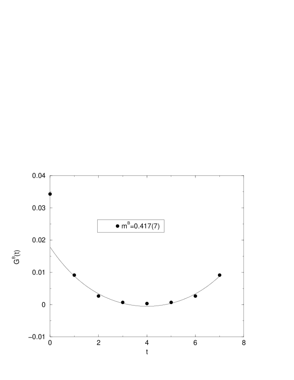
Figure 1: $G^{B}(t)$ for $\alpha=2$, $L=8$

Figure 2: $G^{F}_{01}(t)$ for $\alpha=2$, $L=8$

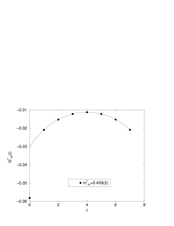
Figure 3: $G^{F}_{00}(t)$ for $\alpha=2$, $L=8$

We are currently extending these simulations to larger $\alpha$ and bigger lattices to study the approach to the continuum limit. Notice that a great deal is known theoretically about the mass spectrum of this model in the continuum [32] and it would be very interesting to check the results of our simulations against this work. Furthermore, it is possible to write down lattice Ward identities for both the exact and broken supersymmetries. Study of these should give information on the question of the restoration of the full $N=2$ supersymmetry in the limit of vanishing lattice spacing. These questions are also under investigation.

5 Lattice Sigma Models in Four Dimensions

Let us turn now to four dimensions. Again, the appropriate gauge condition $N^{i}\left(\phi\right)=0$ must take the form of a (base space) derivative of the target space bosonic field $\phi^{i}$. To ensure that the corresponding antighost $\eta_{i\alpha}$ and multiplier field $B_{i\alpha}$ possess the correct numbers of degrees of freedom this gauge condition should employ some projector to enforce a self-duality condition. In four dimensions this condition should reduce the number of degrees of freedom by a factor of four. In two dimensions the projector depended on an almost complex structure for both base and target spaces both of which were required to be Kähler. The local complex structure associated with a Kähler manifold then ensured that the ghost-antighost action could be reinterpreted as action for Dirac fermions in a chiral representation. In the same way a local almost quaternionic structure is necessary to allow for a representation of the four dimensional Dirac gamma matrix algebra. Manifolds with an almost quaternionic structure possess three independent tensors $\left(J^{a}\right)^{i}_{j}\;a=1\ldots 3$ satisfying the quaternionic algebra

$$J^{a}J^{b}=-\delta^{ab}I+\epsilon^{abc}J^{c}$$ (51)

In terms of these tensors the projector we need looks like [22]

$${P^{i\alpha}_{j\beta}}^{+}=\frac{1}{4}\left(\delta^{i}_{j}\delta^{\alpha}_{\beta}+\left(J^{a}\right)^{i}_{j}\left(j^{a}\right)^{\alpha}_{\beta}\right)$$ (52)

Here, the tensors $J^{a}$ are almost complex structures in the target space and $j^{a}$ are the corresponding base space quantities. The gauge condition in the continuum now reads

$$N^{i\alpha}={P^{i\alpha}_{j\beta}}^{+}\partial^{\beta}\phi^{j}$$ (53)

and as before the antighost and multiplier fields are required to be self-dual under the action of this projector

$$P^{+}\eta=\eta$$ (54)

In a way similar to two dimensions the requirement that the self-duality conditions are compatible with the BRST symmetry requires all three almost complex structures to be covariantly constant. Four dimensional manifolds admitting three such covariantly constant tensors are called hyperKähler.

It is straightforward to find an action corresponding to fixing this gauge condition

$$\xi S=\alpha\delta\int d^{4}\sigma\sqrt{h}\eta_{i\alpha}\left(N^{i\alpha}-\frac{1}{8}B^{i\alpha}\right)$$ (55)

Carrying out the variation and integrating out the multiplier field (taking into account the self-duality condition) yields the following on shell action

$$S = \alpha\int d^{4}\sigma\sqrt{h}\left(\frac{1}{2}h^{\alpha\beta}g_{ij}\partial_{\alpha}\phi^{i}\partial_{\beta}\phi^{j}+\frac{1}{2}\left(j^{a}\right)^{\alpha\beta}\left(J^{a}\right)_{ij}\partial_{\alpha}\phi^{i}\partial_{\beta}\phi^{j}\right.$$ (56)

$$- \left.h^{\alpha\beta}g_{ij}\eta^{i}_{\alpha}D_{\beta}\psi^{j}+\frac{1}{16}R_{ijkl}h^{\alpha\beta}\eta^{i}_{\alpha}\eta^{j}_{\beta}\psi^{k}\psi^{l}\right)$$

Notice again the presence of the base space covariant derivative in the ghost-antighost term. For hyperKähler manifolds the term in the bosonic action containing the tensors $J^{a}$ and $j^{a}$ is again a topological invariant. It is possible to untwist this model to produce a Lorentz invariant theory of Dirac fermions in a way completely analogous to the two dimensional case. To make this explicit it is convenient to introduce a notation that naturally emphasizes the quaternionic nature of the hyperKähler space.

First, group the original $4N$ target fields in sets of four

$$\underbrace{\phi^{1},\phi^{2},\phi^{3},\phi^{4}}_{\Phi^{I},I=1},\underbrace{\phi^{5},\phi^{6},\phi^{7},\phi^{8}}_{\Phi^{I},I=2},...,\underbrace{\phi^{4N-3},\phi^{4N-2},\phi^{4N-1},\phi^{4N}}_{\Phi^{I},I=N}$$ (57)

then the gauge condition condition, ${P^{i\alpha}_{j\beta}}^{+}\partial^{\beta}\phi^{j}=0$ can be rewritten (locally) as

$$\left\{\begin{array}[]{ccc}\partial_{\mu}\Phi^{I}_{\mu}&=&0\\ \partial_{\mu}\Phi^{I}_{\nu}-\partial_{\nu}\Phi^{I}_{\mu}-\epsilon_{\mu\nu\alpha\beta}\partial_{\alpha}\Phi^{I}_{\beta}&=&0\end{array}\right.$$ (60)

($\Phi^{I}_{\mu}$ really means $\phi^{4*(I-1)+\mu}$ with $I=1,...,N$ and $\mu=1,2,3,4$). To see that this is true let us choose the following representation for the $J^{a}$’s (likewise for the $j^{a}$’s)

$$\begin{array}[]{ccc}J^{1}=I=\left(\begin{array}[]{cc}i\sigma_{2}&0\\ 0&i\sigma_{2}\end{array}\right)&J^{2}=J=\left(\begin{array}[]{cc}0&-\sigma_{1}\\ \sigma_{1}&0\end{array}\right)&J^{3}=K=\left(\begin{array}[]{cc}0&-\sigma_{3}\\ \sigma_{3}&0\end{array}\right)\end{array}$$ (68)

Equations (60) are equivalent to the Cauchy-Fueter equations that generalize to four dimensions the Cauchy-Riemann equations of two dimensions [22]. Finally let us adopt quaternionic or hyper-Kähler coordinates by defining

$$\begin{array}[]{lr}\Phi^{I}=-I\Phi^{I}_{1}-J\Phi^{I}_{2}-K\Phi^{I}_{3}+\Phi^{I}_{4}\;{\rm and}\;\partial_{+}=I\partial_{1}+J\partial_{2}+K\partial_{3}+\partial_{4}\end{array}$$ (69)

then equations (60) for the gauge condition take the simple form,

$$\partial_{+}\Phi^{I}=0$$ (70)

Solutions to this equation define so-called triholomorphic functions. The action for the 4D model may then be written in a way analogous to the two dimensional case eqn. 25 by allowing all fields to take values in the quaternions and recognizing that a single quaternionic antighost (and its conjugate) $\eta^{M}_{+}=\eta^{M}_{4}+I\eta^{M}_{1}+J\eta^{M}_{2}+K\eta^{M}_{3}$ survives the self-dual projection.

The physical interpretation of this model necessitates untwisting. The procedure mimics the 2D case. First, it is easy to show that the solutions to the 4D gauge condition correspond to solutions of the Weyl equation for right handed spinors just as in the two dimensional case [22]. Indeed, if we take the chiral Euclidean representation of the four dimensional Dirac matrices,

$$\begin{array}[]{cc}\gamma_{i}=\left(\begin{array}[]{cc}0&-i\sigma_{i}\\ i\sigma_{i}&0\end{array}\right)&\gamma_{4}=\left(\begin{array}[]{cc}0&1\\ 1&0\end{array}\right)\end{array}$$ (76)

the free Dirac operator again becomes simply

$$\gamma.\partial=\left(\begin{array}[]{cc}0&\partial_{+}\\ \partial_{-}&0\end{array}\right)$$ (77)

(where $\partial_{-}=-I\partial_{1}-J\partial_{2}-K\partial_{3}+\partial_{4}$) and we adopt a common representation of the quaternionic structure in terms of the Pauli matrices $I=-i\sigma_{1}$, $J=-i\sigma_{2}$ and $K=-i\sigma_{3}$. Then the action of this operator on a right handed Weyl spinor,

$$\Psi^{I}=\left(\begin{array}[]{c}0\\ 0\\ \Psi^{I}_{1}\\ \Psi_{2}^{I}\end{array}\right)$$ (78)

with,

$$\Psi^{I}_{1} = \Phi^{I}_{4}+i\Phi^{I}_{3}$$

$$\Psi^{I}_{2} = -\Phi^{I}_{2}+i\Phi^{I}_{1}$$ (79)

again just yields the set of equations (60). Thus, the local quaternionic structure of the hyperKähler target space automatically allows us to encode the Clifford algebra of the Dirac matrices and ensures that the ghost and antighost field correspond to the chiral components of a single Dirac fermion. Thus the untwisted model corresponds to the usual $N=2$ theory based on hyper-multiplets [1]

As with the one and two dimensional models it is trivial to discretize this theory while preserving the twisted supersymmetry by simply replacing the derivative operator appearing the gauge condition eqn. 53 by a symmetric difference operator. Such a choice will give rise to both bosonic and fermionic doublers. To remove such states from the spectrum we again need to add a Wilson term in the form of a simple mass operator to the theory. By analogy with the two-dimensional case it would seem that this would only be possible if the target space of the model admits a triholomorphic Killing vector linear in the field. Several examples of such theories are discussed in [28] for hyperKähler manifolds. For such manifolds we can add a Wilson type operator of the form $m_{W}\phi$ while maintaining the Q-exactness of the lattice action.

Following the arguments given earlier the exact supersymmetry will help protect the theory against radiative corrections. Indeed, as in two dimensions, the 4D lattice model will possess three additional discrete symmetries corresponding to acting on the spinors of the theory by each of the three independent complex structures. In the continuum these additional discrete symmetries generate additional supersymmetries. Clearly the requirement that the lattice effective action respect these additional symmetries will force the target manifold to remain hyperKähler under renormalization. This in turn should ensure the full $N=2$ supersymmetry is achieved at large correlation length without further fine tuning.

6 Conclusions

In this paper we have shown how sigma models in one, two and four dimensions with $N=2$ supersymmetry may be discretized in a way which preserves an exact supersymmetry. The argument relies on the well known twisting procedure used to produce topological field theories in the continuum. Here, this argument is turned around and topological constructions are used to generate twisted supersymmetric theories which may then be discretized while preserving an exact (twisted) supersymmetry. The twisted supersymmetry takes the form of a BRST symmetry and the resulting twisted supersymmetric action resembles a gauge fixing term. Notice that while the method we use to construct our lattice actions parallels continuum topological field theory constructions our theories are not topological. They are to be regarded as simply relabeled forms of conventional supersymmetric actions. Indeed, we have untwisted the models explicitly to reveal the physical fermion interpretation. The ghost and anti-ghost fields just correspond to different chiral components of a Dirac fermion field. Notice that from the point of view of simulation this untwisting procedure is somewhat unnecessary - the twisted fields generate precisely the same fermion determinant as the physical fields and it is only this object that we must replicate in any simulation.

The models we construct are local and, at least for target spaces possessing suitable holomorphic Killing vectors, can be rendered free of doubling problems while preserving the Q-exactness of the lattice action. Our preliminary numerical results for the $CP^{1}$ model lend support to these claims. Furthermore, it seems plausible (though we have no proof) that the restoration of Poincaré invariance leads to a restoration of target space reparametrization invariance in these theories. If this is so then we have argued that the exact supersymmetry together with certain discrete symmetries should automatically lead to a restoration of full $N=2$ supersymmetry in the continuum limit without additional fine tuning. We are currently investigating these issues in more detail.

Of course one of the most important questions is whether these ideas may be extended to theories with a gauge symmetry. In the continuum it is indeed possible to construct twisted versions of a variety of super Yang Mills model (the original example being afforded by $N=2$ theory in four dimensions [18]). However, there is an important distinction between these twisted gauge models and both the sigma models described here and the Wess-Zumino models that were considered earlier [15]. The relevant BRST symmetry is now nilpotent only up to gauge transformations – so if we want to latticize such models it appears we must be careful to preserve gauge invariance. While this manuscript was being prepared we received a preprint [33] in which significant progress in this direction had been achieved.

Appendix A Appendix

In this appendix we want to show that

$$\delta^{2}\eta_{i} = 0$$

$$\delta^{2}B_{i} = 0$$ (80)

indeed from (2),

$$\delta^{2}\eta_{i} = \xi(\delta B_{i}-\delta\eta_{j}\Gamma^{j}_{ik}\psi^{k}-\eta_{j}\delta\Gamma^{j}_{ik}\psi^{k})$$

$$= \xi\left\{\chi(B_{j}\Gamma^{j}_{ik}\psi^{k}-\frac{1}{2}\eta_{j}R^{j}_{\;ilk}\psi^{l}\psi^{k})-\chi(B_{j}-\eta_{l}\Gamma^{l}_{jm}\psi^{m})\Gamma^{j}_{ik}\psi^{k}-\eta_{j}\partial_{m}\Gamma^{j}_{ik}\chi\psi^{m}\psi^{k}\right\}$$

$$= -\frac{1}{2}\xi\chi\eta_{j}R^{j}_{\;ilk}\psi^{l}\psi^{k}+\xi\chi\eta_{j}(\Gamma^{j}_{lm}\Gamma^{l}_{ik}+\partial_{m}\Gamma^{j}_{ik})\psi^{m}\psi^{k}$$

but,

$$(\Gamma^{j}_{lm}\Gamma^{l}_{ik}+\partial_{m}\Gamma^{j}_{ik})\psi^{m}\psi^{k} = \frac{1}{2}(\partial_{m}\Gamma^{j}_{ik}-\partial_{k}\Gamma^{j}_{im}+\Gamma^{j}_{lm}\Gamma^{l}_{ik}-\Gamma^{j}_{lk}\Gamma^{l}_{im})\psi^{m}\psi^{k}$$ (81)

$$= \frac{1}{2}R^{j}_{\;imk}\psi^{m}\psi^{k}$$

where $\{\psi^{m},\psi^{k}\}=0$ has been used. Thus,

$$\delta^{2}\eta_{i} = -\frac{1}{2}\xi\chi\eta_{j}R^{j}_{\;ilk}\psi^{l}\psi^{k}+\frac{1}{2}\xi\chi\eta_{j}R^{j}_{\;ilk}\psi^{l}\psi^{k}$$ (82)

$$= 0$$

now consider $\delta^{2}B_{i}$,

$$\delta^{2}B_{i} = \xi\left\{\delta B_{j}\Gamma^{j}_{ik}\psi^{k}+B_{j}\delta\Gamma^{j}_{ik}\psi^{k}-\frac{1}{2}\delta\eta_{j}R^{j}_{\;ilk}\psi^{l}\psi^{k}-\frac{1}{2}\eta_{j}\delta R^{j}_{\;ilk}\psi^{l}\psi^{k}\right\}$$ (83)

$$= \xi\left\{\chi(B_{l}\Gamma^{l}_{jm}\psi^{m}-\frac{1}{2}\eta_{n}R^{n}_{\;jlm}\psi^{l}\psi^{m})\Gamma^{j}_{ik}\psi^{k}+B_{j}\partial_{m}\Gamma^{j}_{ik}\chi\psi^{m}\psi^{k}\right.$$

$$\left.-\frac{1}{2}\chi(B_{j}-\eta_{n}\Gamma^{n}_{js}\psi^{s})R^{j}_{\;ilk}\psi^{l}\psi^{k}-\frac{1}{2}\eta_{j}\partial_{m}R^{j}_{\;ilk}\chi\psi^{m}\psi^{l}\psi^{k}\right\}$$

$$= \xi\chi B_{j}(\Gamma^{j}_{lm}\Gamma^{l}_{ik}+\partial_{m}\Gamma^{j}_{ik})\psi^{m}\psi^{k}-\frac{1}{2}\xi\chi B_{j}R^{j}_{\;ilk}\psi^{l}\psi^{k}$$

$$+\frac{1}{2}\xi\chi\eta_{j}(\partial_{m}R^{j}_{\;ilk}+R^{j}_{\;nlm}\Gamma^{n}_{ik}+\Gamma^{j}_{nm}R^{n}_{\;ilk})\psi^{m}\psi^{l}\psi^{k}$$

using (81), the two first terms cancel each other. The last term can be written as,

$$\eta_{j}(\partial_{m}R^{j}_{\;ilk}+R^{j}_{\;nlm}\Gamma^{n}_{ik}+\Gamma^{j}_{nm}R^{n}_{\;ilk})\psi^{m}\psi^{l}\psi^{k}=\eta_{j}(\partial_{m}R^{j}_{\;ilk}-\Gamma^{n}_{im}R^{j}_{\;nlk}+\Gamma^{j}_{nm}R^{n}_{\;ilk})\psi^{m}\psi^{l}\psi^{k}$$

(where we used the anti-symmetry of the Grassman’s),

$$\hskip 72.26999pt=\eta_{j}(\partial_{m}R^{j}_{\;ilk}+\Gamma^{j}_{nm}R^{n}_{\;ilk}-\Gamma^{n}_{im}R^{j}_{\;nlk}-\Gamma^{n}_{ml}R^{j}_{\;ink}-\Gamma^{n}_{mk}R^{j}_{\;iln})\psi^{m}\psi^{l}\psi^{k}$$ (84)

(as the two added terms vanish when contracted with $\psi^{m}\psi^{l}\psi^{k}$),

$$= \eta_{j}\nabla_{m}R^{j}_{ilk}\psi^{m}\psi^{l}\psi^{k}$$ (85)

$$= \frac{1}{3}\eta_{j}(\nabla_{m}R^{j}_{ilk}+\nabla_{l}R^{j}_{ikm}+\nabla_{k}R^{j}_{iml})\psi^{m}\psi^{l}\psi^{k}$$

$$= 0$$

(by Bianchi identity). Thus $\delta^{2}=0$ i.e. is a nilpotent operation on the multiplet $(\phi,\eta,B,\psi)$.