On practical problems to compute the ghost propagator
in $SU(2)$ lattice gauge theory

Abstract

In $SU(2)$ lattice pure gauge theory we study numerically the dependence of the ghost propagator $G(p)$ on the choice of Gribov copies in Lorentz (or Landau) gauge. We find that the effect of Gribov copies is essential in the scaling window region, however, it tends to decrease with increasing $\beta$. On the other hand, we find that at larger $\beta$-values very strong fluctuations appear which can make problematic the calculation of the ghost propagator.

I Introduction

The nonperturbative study of the ghost propagator is of great interest for the understanding of the mechanism of confinement. The Kugo-Ojima confinement criterium Ojima ; Kugo-Ojima is formulated in terms of the ghost propagator $G^{ab}(p)$ at $p\to 0$ and expresses the absence of colored states from the spectrum of physical states. Moreover, confinement of gluons has been related more directly to the suppression of the gluon propagator in the limit $p\to 0$ Gribov . In both cases, the propagator in question is defined in the Landau (or Lorentz) gauge.

In a series of papers Zwanziger Zwanziger-1 has suggested that this behavior might result from the restriction of the fields in the transversal plane $\Gamma=\{A:\partial_{\mu}A_{\mu}=0\}$ to the Gribov region $\Omega=\{A:\partial_{\mu}A_{\mu}=0,M\geq 0\}$, where the Faddeev-Popov operator $~{}M~{}$ is non-negative.

From studies of the coupled Dyson-Schwinger equations for gluons and ghosts Smekal-Alkofer-Hauck ; Alkofer-Smekal it is well-known that the infrared behaviour of gluon and ghost propagators is closely related Alkofer-Watson : the gluon propagator $D^{ab}_{\mu\nu}(p)=(\delta_{\mu\nu}-p_{\mu}p_{\nu}/p^{2})~{}Z_{gl}(p^{2})/p^{2}$ is damped in the infrared like $Z_{gl}(p^{2})\propto(p^{2})^{2\kappa}$, while the ghost propagator $G^{ab}(p)=\delta^{ab}~{}G(p)=\delta^{ab}~{}Z_{gh}(p^{2})/p^{2}$ is more singular than the free propagator, $Z_{gh}(p^{2})\propto(p^{2})^{-\kappa}$. In a particular truncation scheme $\kappa=0.595$ has been determined IR-exponent ; Zwanziger-4 .

There are only relatively few previous lattice studies of the ghost propagator Suman-Schilling ; Cucchieri-1 ; Nakajima-Furui ; Bloch-Cucchieri-Langfeld-Mendez , in contrast to numerous investigations of the gluon propagator gluon-propagator-1 ; gluon-propagator-2 ; gluon-propagator-3 . As for the latter, is not yet clear from the lattice open-question whether $Z_{gl}(p^{2})/p^{2}\to 0$ or $\neq 0$ with $p^{2}\to 0$ . The lattice volumes might still be insufficient to decide this question. The singular behavior of $Z_{gh}(p^{2})$ is seen to become stronger with increasing volume Cucchieri-1 . This supports the expectation Zwanziger-3 that the sample of physically important gauge field configurations $A\in\Gamma$, which constitutes the Euclidean functional integral, in the thermodynamical limit $V\to\infty$ is concentrating towards the edge of the Gribov region, the first Gribov horizon $\partial\Omega$ where the lowest non-vanishing eigenvalue of the Faddeev-Popov operator is approaching zero. This statement is the content of Zwanziger’s horizon condition Zwanziger-3 ; Zwanziger-Schaden which can be related to the Kugo-Ojima criterion.

All this is complicated by the non-uniqueness, first pointed out by Gribov Gribov , of the intersection with $\Gamma$ of the gauge orbit $A^{g}$ of any gauge field $A$, even if restricted to the Gribov region $\Omega$. Practically, the Landau gauge is implemented by maximizing (with respect to gauge transformations $g$) a certain gauge functional. Usually, such a problem leads to more than a single maximum, which are gauge copies (Gribov copies) of each other, hence to a non-unique definition of gauge dependent observables. Thus, in a lattice investigation one has to determine which observables are really subject to the so-called Gribov problem which reflects the dependence of an observable on the restriction (if possible) to the copy corresponding to the absolute maximum of the gauge functional. More precisely, one has to study whether this dependence disappears when one is approaching the continuum and/or infinite volume limit. Otherwise this would indicate the persistence of a real Gribov problem to which Gribov has drawn the attention. On the lattice, the structure of the Gribov region has been closer investigated under this aspect only by Cucchieri Cucchieri-2 some years ago.

Here we are mainly dealing with the infrared behavior of the calculated ghost propagator. In the result of a study for $SU(2)$ gluodyamics Cucchieri-1 , Cucchieri came to the conclusion that the ghost propagator depends on the selection of the highest among more and more maxima of the gauge functional while the gluon propagator does not depend. This study was restricted on one hand to the strong coupling region ($\beta=0.0$, $0.8$, $1.6$) where these observations apply, and $\beta=2.7$ where no gauge copy dependence was seen at all. These $\beta$ values are outside the physically interesting scaling region. In a more recent paper Bloch-Cucchieri-Langfeld-Mendez , it has been reported that the gauge copy dependence of the ghost propagator in the more interesting scaling region (at $\beta=2.15$, $2.2$, $2.3$ and $2.4$ for lattices $16^{3}\times 32$) has been found to be within the statistical errors, on a level which is called Gribov noise.

In the present paper we reanalyse the scaling region at $\beta=2.2$, $2.3$, $2.4$, $2.5$ and $2.6$ for lattices $8^{4}$ and $16^{4}$ by comparing two ensembles of gauge-fixed field configurations. One ensemble (”fc”) consists of an arbitrary maximum (usually the first being found), and the other consists of the best (relative) maximum (”bc”) among $N_{copy}$ local maxima of the gauge functional. We find that the difference of the ensemble averages of the ghost propagator for the lowest non-vanishing lattice momentum between the two ensembles does not vanish, except for the highest $\beta$ value. Hence the Gribov problem remains a serious obstacle for a unique definition of the $SU(2)$ ghost propagator in the scaling region. More serious is an unexpected observation in the higher-$\beta$ region. We find an intermittent behavior of the ghost propagator estimator for the lowest non-vanishing momentum, signalled by anomalously large, isolated fluctuations of the ghost propagator $G(p_{min})$ (see below) within the time history of uncorrelated configurations. We stress already here that this behavior is not a Gribov copy problem since the anomalous peaks of $G(p_{min})$ are observed both for the first and the best Gribov copy, entering the ensembles ”fc” and ”bc”, respectively. We have tested whether this is correlated with various infrared observables. For the time being, two hypothetic causes must be excluded as a viable explanation of the phenomenon.

In Section 2 we recall the definition of the gluon field $A_{\mu}$, the definition of the Lorentz (or Landau) gauge, the structure of the Faddeev-Popov operator and the definition of the ghost propagator. Details of the simulations, the gauge fixing and the observation of Gribov copies are reported in Section 3. In Section 4 we discuss the results on the ghost propagator. We conclude in Section 5.

II Faddeev-Popov operator and ghost propagator

II.1 Definition of the gluon field and Faddeev-Popov operator

For the Monte Carlo generation of ensembles of non-gauge-fixed gauge field configurations we use the standard Wilson action Wilson , which for the case of an $SU(N)$ gauge group is written

$$S = \beta\sum_{x}\sum_{\mu>\nu}\left[1-\frac{1}{N}~{}\mbox{Re}~{}\mbox{Tr}\Bigl{(}U_{x\mu}U_{x+\mu;\nu}U_{x+\nu;\mu}^{\dagger}U_{x\nu}^{\dagger}\Bigr{)}\right]\;;$$ (1)

$$\beta=2N/g_{0}^{2}\;.$$

Here $g_{0}$ is a bare coupling constant and $U_{x\mu}\in SU(N)$ are the link variables. The field variables $U_{x\mu}$ transform as follows under gauge transformations $g_{x}$ :

$$U_{x\mu} \stackrel{{\scriptstyle g}}{{\mapsto}} U_{x\mu}^{g}=g_{x}^{\dagger}U_{x\mu}g_{x+\mu}\;;\qquad g_{x}\in SU(N)\;.$$ (2)

For $SU(2)$ gauge links $U_{x\mu}$, a standard definition Mandula-Ogilvie of the lattice gauge field (vector potential) ${\cal A}_{x+\hat{\mu}/2,\mu}$ is

$${\cal A}_{x+\hat{\mu}/2,\mu}=\frac{1}{2i}~{}\Bigl{(}U_{x\mu}-U_{x\mu}^{\dagger}\Bigr{)}\;.$$ (3)

Therefore, for $SU(2)$, the link can be written

$$U_{x\mu} = b^{0}_{x\mu}~{}{\hat{1}}+i~{}{\vec{b}}_{x\mu}~{}{\vec{\sigma}}=b^{0}_{x\mu}~{}{\hat{1}}+i~{}{\cal A}_{x+\hat{\mu}/2;\mu}\;;$$

$$b^{0}_{x\mu} = \frac{1}{2}~{}\mbox{Tr}~{}U_{x\mu}\;.$$ (4)

In lattice gauge theory the usual choice of the Landau gauge condition is Mandula-Ogilvie

$$(\partial{\cal A})_{x}=\sum_{\mu=1}^{4}\left({\cal A}_{x+\hat{\mu}/2;\mu}-{\cal A}_{x-\hat{\mu}/2;\mu}\right)=0\;,$$ (5)

which is equivalent to finding an extremum of the gauge functional

$$F_{U}(g)=\frac{1}{4V_{4}}~{}\sum_{x\mu}~{}\frac{1}{N}~{}\mbox{Re}~{}\mbox{Tr}~{}U^{g}_{x\mu}\;$$ (6)

with respect to gauge transformations $g_{x}~{}$. After replacing $U\Rightarrow U^{g}$ at the extremum the gauge condition (5) is satisfied. In what follows this gauge is referred to as Landau gauge.

The lattice expression of the Faddeev-Popov operator $M^{ab}$ corresponding to $M^{ab}=-\partial_{\mu}D^{ab}_{\mu}$ in the continuum theory (where $D^{ab}_{\mu}$ is the covariant derivative in the adjoint representation) is given by

$$M^{ab}_{xy}=\sum_{\mu}~{}\Bigl{\{}\left(\bar{S}^{ab}_{x\mu}+\bar{S}^{ab}_{x-\hat{\mu};\mu}\right)~{}\delta_{x;y}\Bigr{.}$$

$$\Bigl{.}-\left(\bar{S}^{ab}_{x\mu}-\bar{A}^{ab}_{x\mu}\right)~{}\delta_{y;x+\hat{\mu}}\Bigr{.}$$ (7)

$$\Bigl{.}-\left(\bar{S}^{ab}_{x-\hat{\mu};\mu}+\bar{A}^{ab}_{x-\hat{\mu};\mu}\right)~{}\delta_{y;x-\hat{\mu}}\Bigr{\}}$$

where

$$\bar{S}^{ab}_{x\mu}=\delta^{ab}~{}\frac{1}{2}~{}\mbox{Tr}~{}U_{x\mu}\;;\quad\bar{A}^{ab}_{x\mu}=-\frac{1}{2}~{}\epsilon^{abc}~{}A_{x+\hat{\mu}/2;\mu}^{c}\;.$$ (8)

From the form (II.1) it follows that a trivial zero eigenvalue is always present, such that at the Gribov horizon $\partial\Gamma$ the first non-trivial zero eigenvalue appears. Conversely, it is easy to see that for constant field configurations, with $b^{0}_{x\mu}=\bar{b}^{0}_{\mu}$ and $b^{a}_{x\mu}=\bar{b}^{a}_{\mu}$ independent of $x$, there exist eigenmodes of $M$ with a vanishing eigenvalue. Thus, if the Landau gauge is properly implemented, $M[U]$ is a symmetric and semi-positive definite matrix.

II.2 Ghost propagator

The ghost propagator $G^{ab}(x,y)$ is defined as Zwanziger-3 ; Suman-Schilling

$$G^{ab}(x,y)=\delta^{ab}~{}G(x-y)\equiv\Bigl{<}\,\left(\,M^{-1}\,\right)^{a\,b}_{x\,y}[U]\,\Bigl{>}\;,$$ (9)

where $M[U]$ is the Faddeev-Popov operator. Note that the ghost propagator becomes translational invariant (i.e., dependent only on $x-y$) and diagonal in color space only in the result of averaging over the ensemble of gauge-fixed representants (first or best gauge-fixed copies) of the original Monte Carlo gauge configurations. The ghost propagator in momentum space can be written as

$$G(p)\,=\,\frac{1}{3V}\sum_{x\mbox{,}\,y}e^{-2\pi i\,p\cdot(x-y)}\Bigl{<}\,\left(\,M^{-1}\,\right)^{a\,a}_{x\,y}[U]\,\Bigl{>}\;,$$ (10)

where $V=L^{4}$ is the lattice volume, and the coefficient $\frac{1}{3V}$ is taken for a full normalization, including the indicated color average over $a=1,..,3$.

We mentioned above that $M[U]$ is a symmetric and semi-positive definite matrix. In particular, this matrix is positive-definite in the subspace orthogonal to constant vectors. The latter are zero modes of $M[U]$. Therefore, it can be inverted by using a conjugate-gradient method, provided that both the source $\psi^{a}(y)$ and the initial guess of the solution are orthogonal to zero modes. As the source we adopted the one proposed by Cucchieri Cucchieri-1 :

$$\psi^{a}(y)\,=\,\delta^{ac}\,e^{2\pi i\,p\cdot y}\qquad p\neq(0,0,0,0)\;,$$ (11)

for which the condition $\sum_{y}\,\psi^{a}(y)\,=\,0$ is automatically imposed. Choosing the source in this way allows to save computer time since, instead of the summation over $x$ and $y$ in Eq. (10), only the scalar product of $M^{-1}\psi$ with the source $\psi$ itself has to be evaluated. In general, the gauge fixed configurations can be used in a more efficient way when the inversion of $M$ is done on sources for $c=1,..,3$ such that the (adjoint) color averaging, formally required in Eq. (10), will be explicitely performed.

III Simulation details

The numerical simulations have been done for $SU(2)$ pure gauge theory using the standard Wilson action, for lattice volumes $L^{4}$ with $L=8$ and $L=16$. At a given lattice size $L$ for each $\beta$ value we have generated $N_{conf}$ independent mother configurations, for which the Landau gauge was fixed $N_{copy}=20$ times, each time starting from a random gauge transformation of the mother configuration, obtaining in this way $N_{copy}$ Landau-gauge fixed copies.

Two consecutive configurations (considered as independent) were separated by 100 and 200 sweeps for lattice sizes $8^{4}$ and $16^{4}$, respectively. Each sweep consisted of one local heatbath update followed by 4 or 8 microcanonical updates Adler for $8^{4}$ or $16^{4}$ lattices. In all our runs we have measured the integrated autocorrelation time for the plaquette, for the Polyakov loop and for the ghost propagator (separately for each momentum $p$). In all cases, the relation $\tau_{int}\sim 0.5$ was observed, showing that the consecutive configurations are effectively independent.

The actual measurements of the ghost propagator were done for the ”first”, i.e. in fact an arbitrary gauge copy and for the ”best” one among the $N_{copy}$ copies. If the first copy turned out to be the best, the ghost propagator was measured only once, and the result simultaneously entered the two different gauge-fixed ensemble averages. In the following the two ensembles are labelled ”fc” and ”bc”, refering to the first or the best gauge copy, respectively. In Table 1 we give, for each set of simulation parameters $(L,\beta)$, the number of times the first copy produced turned not out to be the best, i.e., did not correspond to the relative maximum of $F_{U}(g_{i})$ among the $N_{copy}$ copies.

As the gauge fixing procedure we used standard Los Alamos type overrelaxation with $\omega=1.7$. The iterations have been stopped when the following transversality condition was satisfied:

$$\max_{x\mbox{,}\,a}\,\Big{|}\sum_{\mu=1}^{4}\left(A_{x+\hat{\mu}/2;\mu}^{a}-A_{x-\hat{\mu}/2;\mu}^{a}\right)\Big{|}\,<\,\epsilon_{lor}\;.$$ (12)

We used the parameters $\epsilon_{lor}=10^{-10}$ or $10^{-9}$ for lattice size $8^{4}$ or $16^{4}$, respectively. In our test runs it was found that further decreasing $\epsilon_{lor}$ does not affect the results for the ghost propagator. Also it was checked that these values of $\epsilon_{lor}$ are sufficient for identifying, according only to the values of $F_{U}(g_{i})$, Gribov copies which are actually global gauge transformations of each other and conversely for distinguishing this from the case of actually inequivalent lattice Gribov copies.

In Table 1, for each set of simulation parameters $(L,\beta)$, we present also the number of configurations for which Gribov copies have been found and the total number of different Gribov copies.

The momenta $p$ for the propagator $G(p)$ were taken with all spatial components put equal to zero: $p=(0,0,0,k_{4}/L)$, where $k_{4}$ was restricted to $k_{4}=1,2,3,4$.

size	$\beta$	$N^{conf}_{multiple~{}copies}/N^{conf}$	$N^{copies}_{nonequiv}/N^{copies}_{total}$	$N_{fc\neq bc}$
$8^{4}$	1.6	500 / 500	8263 / 10000	446
	2.0	490 / 500	4431 / 10000	354
	2.1	468 / 500	3460 / 10000	311
	2.2	426 / 500	2180 / 10000	235
	2.3	301 / 500	1364 / 10000	150
	2.4	184 / 500	877 / 10000	92
$16^{4}$	2.0	25 / 25	500 / 500	25
	2.1	25 / 25	500 / 500	25
	2.2	25 / 25	500 / 500	23
	2.3	25 / 25	494 / 500	25
	2.4	25 / 25	337 / 500	23
	2.5	24 / 25	169 / 500	14

Table 1: The Table shows in the 3rd column the number $N^{conf}_{multiple~{}copies}$ of configurations, for which non-equivalent Gribov copies have actually been obtained, out of a total number $N^{conf}$ of configurations which underwent gauge fixing; in the 4th column the total number $N^{copies}_{nonequiv}$ of non-equivalent Gribov copies out of a total number $N^{copies}_{total}=N^{conf}\times N_{copy}$ of gauge copies under investigation. The last column presents the number of times out of $N^{conf}$ that the first copy was not identical to the best (relative maximum) copy.

$8^{4}$ lattice
$\beta$	$n_{meas}$	Copy	$k_{4}=1$	$k_{4}=2$	$k_{4}=3$	$k_{4}=4$
$1.6$	$500$	bc	$6.58(4)$	$1.327(5)$	$0.628(2)$	$0.501(1)$
$1.6$	$500$	fc	$7.02(6)$	$1.363(5)$	$0.638(1)$	$0.508(1)$
$2.0$	$500$	bc	$5.15(3)$	$1.013(2)$	$0.491(1)$	$0.3970(4)$
$2.0$	$500$	fc	$5.46(9)$	$1.028(3)$	$0.495(1)$	$0.3995(6)$
$2.1$	$500$	bc	$4.62(3)$	$0.920(2)$	$0.4545(6)$	$0.3701(4)$
$2.1$	$500$	fc	$4.89(7)$	$0.935(3)$	$0.4573(8)$	$0.3719(5)$
$2.2$	$500$	bc	$4.06(3)$	$0.823(2)$	$0.4189(4)$	$0.3444(3)$
$2.2$	$500$	fc	$4.26(4)$	$0.833(2)$	$0.4203(5)$	$0.3450(3)$
$2.3$	$500$	bc	$3.60(4)$	$0.744(1)$	$0.3903(3)$	$0.3238(2)$
$2.3$	$500$	fc	$3.65(4)$	$0.747(2)$	$0.3909(4)$	$0.3241(2)$
$2.4$	$500$	bc	$3.38(5)$	$0.691(1)$	$0.3710(4)$	$0.3098(2)$
$2.4$	$500$	fc	$3.47(7)$	$0.692(2)$	$0.3712(4)$	$0.3099(2)$
$16^{4}$ lattice
$\beta$	$n_{meas}$	Copy	$k_{4}=1$	$k_{4}=2$	$k_{4}=3$	$k_{4}=4$
$2.2$	$296$	bc	$20.1(1)$	$3.87(1)$	$1.494(2)$	$0.8078(6)$
$2.2$	$296$	fc	$21.3(1)$	$3.97(1)$	$1.509(2)$	$0.8115(6)$
$2.3$	$270$	bc	$17.3(1)$	$3.29(1)$	$1.303(1)$	$0.7248(4)$
$2.3$	$270$	fc	$18.0(1)$	$3.33(1)$	$1.310(2)$	$0.7268(5)$
$2.4$	$370$	bc	$14.8(1)$	$2.83(1)$	$1.165(1)$	$0.6673(3)$
$2.4$	$370$	fc	$15.6(1)$	$2.87(1)$	$1.171(1)$	$0.6690(3)$
$2.5$	$294$	bc	$13.7(2)$	$2.56(1)$	$1.088(1)$	$0.6353(3)$
$2.5$	$294$	fc	$13.9(2)$	$2.58(1)$	$1.090(1)$	$0.6358(3)$
$2.6$	$229$	bc	$13.6(4)$	$2.41(1)$	$1.043(2)$	$0.6161(5)$
$2.6$	$229$	fc	$13.8(4)$	$2.41(1)$	$1.044(2)$	$0.6164(5)$

Table 2: The ghost propagator $G(p)$ from Eq. (10) as a function of $k_{4}=1,2,3,4$. We have set the momentum $p=(0,0,0,k_{4}/L)$, where $L=8,16$ is the lattice size. The averages over the gauge configurations in Eq. (10) were taken in two different ways: ”fc” means the average taking only the gauge-fixed copy generated first for each configuration, ”bc” means the average over only the best (relative maximum) copy among $20$ different gauge-fixed copies that we have generated.

IV Discussion of the Results

From Table 1 one can learn that at the lattice size $8^{4}$ the fraction of Monte Carlo configurations which are represented by more than one gauge-fixed configurations (among 20 attempts to find copies) drastically begins to decrease at $\beta=2.3$. Parallel to this also the multiplicity of actually different copies among 20 drops down. The decrease of the number of available basins of attraction for the gauge fixing process is a finite-volume effect. For the bigger lattice size ($16^{4}$) one sees that the fraction of Monte Carlo configurations with more than one gauge-fixed configurations practically does not depend on $\beta$. However, the multiplicity of non-equivalent copies among the 20 obtained copies starts to decrease from $\beta=2.3$.

From Table 2 one can see for separate small momenta, how the average value of the ghost propagator differs between the two ways to deal with the Gribov copy problem: to ignore it ($N_{copy}=1$) or to inspect $N_{copy}=20$ copies. For all momenta, the ensemble consisting of the first copies (’fc’) turns out to give slightly larger values than the ensemble including always the best copy (’bc’).

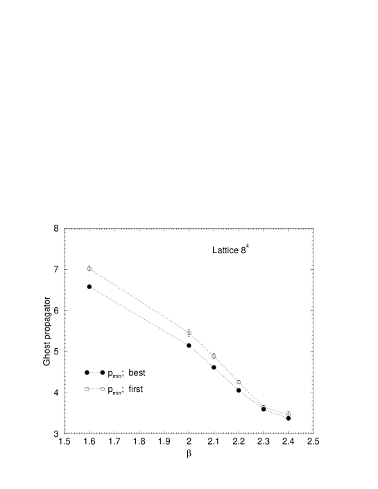
Figure 1: The $\beta$ dependence and Gribov copy sensitivity of the ghost propagator $G(p_{min})$ at minimal momentum $p_{min}$ on the $8^{4}$ lattice. Filled symbols correspond to the ’bc’ ensemble, open symbols to the ’fc’ ensemble (see the text).

For the lowest non-vanishing momentum this is shown in Fig. 1 for the lattice $8^{4}$. It is visible that for $\beta\in[1.5,2.4]$ the difference of $G(p_{min})$ between the two ways of averaging is clearly outside the statistical error.

In Fig. 2, for the bigger lattice $16^{4}$, the ghost propagator values for the two lowest momenta are compared with respect to the dependence on Gribov copies for $\beta\in[2.2,2.6]$. Whereas for the lowest momentum the results resemble those of the smaller lattice, for the second lowest momentum they are practically indistinguishable at the given scale. For increasing $\beta$ the difference becomes of the order of the statistical error (Gribov noise). At $\beta=2.6$ the ghost propagator data even for the lowest momentum fall together within error bars. This indicates that the Gribov problem has disappeared for the ghost propagator there.

Figure 2: The $\beta$ dependence and Gribov copy sensitivity of the ghost propagator $G(p)$ at minimal momentum $p_{min}$ and next-to-minimum momentum $2p_{min}$ on the $16^{4}$ lattice. Filled symbols correspond to the ’bc’ ensemble, open symbols to the ’fc’ ensemble. At $\beta=2.6$ the minimal momentum ghost propagator is sensitive to the inclusion or exclusion of ”exceptional configurations” (see text).

Instead, at $\beta=2.6$ a new problem arises which can be recognized already in Fig. 2 where we also demonstrate how, at $\beta=2.6$, the average for the ghost propagator at the lowest momentum would be influenced by the removal of ”exceptional configurations”. These are signalled as spikes in the Monte Carlo time histories of the corresponding observable shown in Fig. 3 for $\beta=2.6$. Precursors of this phenomenon are visible there at lower $\beta$, too, but for $\beta=2.6$ the effect becomes notable. We notice that these spikes occur in the first as well as in the best gauge-fixed copy. Therefore, the existence of these ”exceptional configurations” is definitely not a result of gauge fixing.

Figure 3: Monte Carlo time histories of the ghost propagator $G(p_{min})$ for various $\beta$ on the $16^{4}$ lattice. The frequency of the occurrence of ”exceptional configurations” increases with higher $\beta$.

In order to explore what the essence of these ”exceptional configurations” is, we have looked for correlations with certain ”toron” excitations on one hand and with different Polyakov loops on the other.

In the first case we followed the procedure applied by Kovacs Kovacs for extracting the toron content of Monte Carlo gauge field configurations . We evaluated for all four directions $\mu$ on the lattice the corresponding holonomies over a $\mu$-slice fixed at $x_{\mu}=1$

$${\cal P}_{\mu}(x)=\prod_{s=0}^{L-1}U_{x+s\hat{\mu};\mu}\;.$$ (1)

We averaged this quantity over the $\mu$-slice,

$$\bar{{\cal P}}_{\mu}=\frac{1}{L^{3}}\sum_{x;x_{\mu}=1}{\cal P}_{\mu}(x)\;.$$ (2)

These gauge dependent quantities were normalized to $SU(2)$ in the usual way

$$\bar{{\cal P}}_{\mu}\Rightarrow\bar{{\cal P}}_{\mu}/\sqrt{\mathrm{det}\bar{{\cal P}}_{\mu}}\;.$$ (3)

Then the anticipated homogeneous toron field is given by links $\bar{U}_{x\mu}$ independent of $x$, which are required to reproduce $\bar{{\cal P}}_{\mu}$ as follows :

$$(\bar{U}_{x\mu})^{L}=\bar{{\cal P}}_{\mu}\;.$$ (4)

The corresponding toron gluon field can be extracted as

$${\cal A}^{toron}_{x+\hat{\mu}/2;\mu}=\frac{1}{2i}~{}\Bigl{(}\bar{U}_{x\mu}-\bar{U}_{x\mu}^{\dagger}\Bigr{)}\;.$$ (5)

We have plotted the time history of the lowest momentum ghost propagator together with the toron observable

$$T_{\mu}=\sum_{a=1}^{3}\mbox{Tr}~{}({{\cal A}}^{toron}_{x+\hat{\mu}/2;\mu})^{2}\;,$$ (6)

defined separately for the four Euclidean directions. We noticed that the previously mentioned spikes (”exceptional configurations”) occur independent of spikes of this toron observable in each of the Euclidean directions. We demonstrate this in Fig. 4 which shows the Monte Carlo history of the lowest-momentum ghost propagator (upper panel) together with the histories of the toron fields $T_{\mu}$ for $\mu=4$ (middle) and $\mu=1$ (lower panel).

Figure 4: Monte Carlo time histories of the ghost propagator $G(p_{min})$ (above) for $\beta=2.6$ on the $16^{4}$ lattice, compared with the histories of the toron fields $T_{4}$ (middle) and $T_{1}$ (below). The fluctuations of the latter have been arbitrarily rescaled and shifted for better visual inspection.

We also checked the Monte Carlo sample for eventual correlations with the average Polyakov loop

$$L_{\mu}=\frac{1}{2}\mbox{Tr}~{}\bar{{\cal P}}_{\mu}\;.$$ (7)

Similarly, we illustrate in Fig. 5 that there are no correlations between the spikes of the lowest momentum ghost propagator with extremal fluctuations of the average Polyakov loop in any of the four directions. Shown in the Fig. 5 are, beside the history of the lowest-momentum ghost propagator (upper panel), the histories of the average Polyakov lines $L_{\mu}$ for $\mu=4$ (middle) and $\mu=1$ (lower panel).

Figure 5: Monte Carlo time histories of the ghost propagator $G(p_{min})$ (above) for $\beta=2.6$ on the $16^{4}$ lattice, compared with the histories of the average Polyakov lines $L_{4}$ (middle) and $L_{1}$ (below). The fluctuations of the latter have been arbitrarily rescaled and shifted for better visual inspection.

V Conclusions

In this work we studied numerically the dependence of the ghost propagator $G(p)$ in pure gauge $SU(2)$ theory on the choice of Gribov copies in Lorentz (or Landau) gauge with the special focus on the physically interesting scaling region. All simulations have been performed on the $~{}8^{4}~{}$ and $~{}16^{4}~{}$ lattices.

We found that the effect of Gribov copies is essential in the scaling window region. Therefore, the Gribov problem remains a serious obstacle for a unique definition of the $SU(2)$ ghost propagator in the scaling region. However, it tends to decrease with increasing $\beta$ values.

Another – and more serious – problem is presented by the unexpected observation, in the higher-$\beta$ region, of anomalously large, isolated fluctuations of the ghost propagator $G(p_{min})$ within the time history of uncorrelated configurations. These strong fluctuations make problematic the calculation of the ghost propagator.

We believe that this problem deserves a more thorough study, in particular how to interpret the relevant configurations. If there is nothing physically wrong with them, much more statistics is necessary to get a reliable result.

Acknowledgment

This work has been supported by the grant INTAS–00–00111 and RFBR grants 02–02–17308 and 99–01–00190. One of us (T. B.) recognizes the support of young scientist’s grant 02-01-06064. E.–M. I. is supported by DFG through the DFG-Forschergruppe ”Lattice Hadron Phenomenology” (FOR 465).

References

- (1) I. Ojima, Nucl. Phys. B 143, 340 (1978).
- (2) T. Kugo and I. Ojima, Prog. Theor. Phys. Suppl. 66, 1 (1979).
- (3) V. N. Gribov, Nucl. Phys. B 139, 1 (1978).
- (4) D. Zwanziger, Nucl. Phys. B 364, 127 (1991); Nucl. Phys. B 378, 525 (1992).
- (5) L. von Smekal, R. Alkofer and A. Hauck, Phys. Rev. Lett. 79, 3591 (1997); L. von Smekal, A. Hauck and R. Alkofer, Ann. Phys. (NY) 267, 1 (1998), Erratum-ibid. 269,182 (1998).
- (6) R. Alkofer and L. von Smekal, Phys. Rept. 353, 281 (2001).
- (7) P. Watson and R. Alkofer, Phys. Rev. Lett. 86, 5239 (2001).
- (8) R. Alkofer, C.S. Fischer and L. von Smekal, Eur. Phys. J. A 17, 773 (2003); Prog. Part. Nucl. Phys. 50, 317 (2003), e-print archive: nucl-th/0301048.
- (9) D. Zwanziger, Phys. Rev. D 65, 094039 (2002); Phys. Rev. D 67, 105001 (2003).
- (10) H. Suman and K. Schilling, Phys. Lett. B 373, 314 (1996).
- (11) A. Cucchieri, Nucl. Phys. B 508, 353 (1997).
- (12) H. Nakajima and S. Furui, Nucl. Phys. B (Proc. Suppl.) 73, 865 (1999); Nucl. Phys. B (Proc. Suppl.) 83, 521 (2000); Nucl. Phys. A 680, 151 (2000); H. Nakajima, S. Furui and A. Yamaguchi, Nucl. Phys. B (Proc. Suppl.) 94, 558 (2001); H. Nakajima and S. Furui, Nucl. Phys. B (Proc. Suppl.) 119, 730 (2003).
-
(13)
J.C.R Bloch, A. Cucchieri, K. Langfeld and T. Mendez,
Nucl. Phys. B (Proc. Suppl.) 119, 736 (2003);
K. Langfeld, J.C.R. Bloch, J. Gattnar, H. Reinhardt, A. Cucchieri and T. Mendes, talk given at 5th International Conference on Quark Confinement and the Hadron Spectrum, Gargnano, Brescia, Italy, 10-14 Sep 2002, edited by N. Brambilla, G. M. Prosperi; River Edge, N.J., World Scientific (2003), pp. 297-299; e-print archive: hep-th/0209173. - (14) J. E. Mandula, Phys. Rept. 315, 273 (1999).
-
(15)
G. Damm, W. Kerler and V.K. Mitrjushkin,
Phys. Lett. B 433, 88 (1998);
A. Cucchieri, Phys. Rev. D 60, 034508 (1999);
K. Langfeld, H. Reinhardt and J. Gattnar, Nucl. Phys. B 621, 131 (2002);
A. Cucchieri, T. Mendes and A. R. Taurines, Phus. Rev. D 67, 091502 (2003). -
(16)
D. B. Leinweber et al. (UKQCD collaboration),
Phys. Rev. D 58, 031501 (1988);
Phys. Rev. D 60, 094507 (1999),
Erratum-ibid. D 61, 079901 (2000);
H. Nakajima and S. Furui, Nucl. Phys. B (Proc. Suppl.) 73, 635 (1999);
F.D.R. Bonnet, P. O. Bowman, D. B. Leinweber and A. G. Williams, Phys. Rev. D 62, 051501 (2000); F.D.R. Bonnet, P. O. Bowman, D. B. Leinweber, A. G. Williams and J. M. Zanotti, Phys. Rev. D 64, 034501 (2001). - (17) see the last two of Ref. gluon-propagator-3
-
(18)
C. Alexandrou, P. de Forcrand and E. Follana,
Phys. Rev. D 65, 114508 (2002);
P. O. Bowman, U. M. Heller, D. B. Leinweber and A. G. Williams, Phys. Rev. D 66, 074505 (2002). - (19) D. Zwanziger, Nucl. Phys. B 412, 657 (1994).
- (20) M. Schaden and D. Zwanziger, in Proceedings of the Workshop on Quantum Infrared Physics, Paris, France, 6-10 Jun 1994, edited by H.M. Fried and B. Muller; River Edge, N.J., World Scientific (1995), pp. 0010-17; e-print archive: hep-th/9410019.
- (21) A. Cucchieri, Nucl. Phys. B 521, 365 (1998).
- (22) K. Wilson, Phys. Rev. D 10, 2445 (1974). .
- (23) J. E. Mandula and M. Ogilvie, Phys. Lett. B 185, 127 (1987).
- (24) S. L. Adler, Nucl. Phys. B (Proc. Suppl.) 9, 437 (1989).
- (25) T. G. Kovacs, Phys. Rev. D 62, 034502 (2000).