UNITU-THEP-17/2003

Center Vortex Model for the Infrared Sector of $SU(3)$ Yang-Mills Theory – Confinement and Deconfinement

M. Engelhardt, M. Quandt, H. Reinhardt^∗

Institut für Theoretische Physik, Universität Tübingen

D–72076 Tübingen, Germany.

The center vortex model for the infrared sector of Yang-Mills theory, previously studied for the $SU(2)$ gauge group, is extended to $SU(3)$. This model is based on the assumption that vortex world-surfaces can be viewed as random surfaces in Euclidean space-time. The confining properties are investigated, with a particular emphasis on the finite-temperature deconfining phase transition. The model predicts a very weak first order transition, in agreement with $SU(3)$ lattice Yang-Mills theory, and also reproduces a consistent behavior of the spatial string tension in the deconfined phase. The geometrical structure of the center vortices is studied, including vortex branchings, which are a new property of the $SU(3)$ case.

1 Introduction

The vortex picture of the Yang-Mills vacuum was initially proposed [1, 2, 3, 4] as a possible mechanism of confinement. It is based on the idea that the presence of vortex flux randomly distributed in space-time is sufficient to disorder Wilson loops to such an extent that an area law behavior of their expectation values is generated. The picture was further elaborated by the Copenhagen group [5], who considered the energetics of vortex formation in the Yang-Mills vacuum, and it was also cast in lattice gauge theory terms [2]. In particular, an alternative confinement criterion based on vortex free energies on the lattice was formulated.

Apart from further developments within the lattice description [6], the vortex picture lay dormant until the advent of new gauge fixing techniques which permit the detection of center vortex structures in lattice Yang-Mills configurations [7, 8]. In essence, one uses the gauge freedom to cast a given gauge configuration as accurately as possible in terms of an appropriate center vortex configuration [9]. In a second step, center projection, one extracts the vortex content by discarding residual deviations from the aforementioned center vortex configuration [7]. Based on this procedure, it was possible to isolate the effects of the resulting center projection vortices on strong interaction phenomena. It was soon realized that these center projection vortices are physical in the sense that their density shows the proper scaling behaviour [7, 10]. Detailed exploration sharpened the understanding of the center gauge fixing techniques [9], also indicating points where care must be taken in their application [11]. Nevertheless, a broad body of evidence now indicates that the infrared properties of Yang-Mills theory can be accounted for in terms of vortex effects; this includes not only the confinement properties (i.e., the original focus of the vortex picture) [7, 10, 12, 13, 14, 15, 16, 17], but also the topological properties [9, 18, 19, 20, 21] determining the axial flavor $U_{A}(1)$ anomaly [22, 23, 21] and the spontaneous breaking of chiral symmetry [22, 8, 24].

These findings suggest that center vortices are the relevant infrared degrees of freedom of Yang-Mills theory. Using that as the basic assumption, a random vortex world-surface model for the infrared sector of Yang-Mills theory was introduced [15] to complement the lattice gauge investigations highlighted above. Initially studied for the $SU(2)$ gauge group, it not only reproduces the confinement properties [15] of $SU(2)$ Yang-Mills theory quantitatively, but also the topological susceptibility [21] and the spontaneous breaking of chiral symmetry [24].

The present work extends the model to the $SU(3)$ gauge group, focusing on the confinement properties. The main physical difference to the $SU(2)$ case is the fact that vortex world-surfaces can branch due to the existence of two types of quantized vortex flux instead of one. This is expected to lead to important phenomenological consequences, such as a change in the order of the finite temperature deconfinement phase transition.

The paper is organized as follows: In section 2, the center vortex model of ref. [15] is revisited and extended to the gauge group $SU(3)$. In section 3, the confinement properties in the parameter space of coupling constants are investigated, yielding a determination of a physical line in that space. The order of the deconfinement phase transition is studied in section 4 and the geometrical structure of the world-surfaces present in the vortex ensemble is investigated in section 5. Section 6 is devoted to the study of vortex branchings. Section 7 contains concluding remarks.

2 Definition of the random vortex world-surface model

2.1 General properties of center vortices

Center vortices are closed lines of chromomagnetic flux in three space dimensions; correspondingly, they are described by two-dimensional closed world-surfaces in four-dimensional space-time. Their flux is quantized according to the center of the underlying gauge group $SU(N)$. To be specific, this means that measuring the flux by evaluating a Wilson loop $\mathcal{C}$ encircling the vortex will result in a center element of $SU(N)$,

$$W[\mathcal{C}]=\frac{1}{N}\mbox{ Tr }{\cal P}\exp\left(i\oint_{\mathcal{C}}A_{\mu}dx_{\mu}\right)\in Z(N)\ .$$ (1)

In the case of the gauge group $SU(2)$ [15], there is one nontrivial center element and, correspondingly, one type of vortex flux; by contrast, in the case of $SU(3)$, there are two nontrivial center elements in addition to the trivial unit element,

$$Z(3)=\left\{1,\,\exp(2\pi i/3),\,\exp(4\pi i/3)\right\}\ .$$ (2)

This means that there are two distinct types of vortex flux. If one denotes the center elements, eq. (2), as

$$z_{q}=\exp(2\pi iq/3)$$ (3)

with the triality $q$ defined modulo 3,

$$q\in\{0,1,2\}$$ (4)

then one can label the two types of vortex flux by associating them with $q=1$ or $q=2$.

It is important to note that reversing the direction of the loop integration in a Wilson loop or, equivalently, reversing the space-time orientation of the vortex flux encircled by a given Wilson loop leads to a complex conjugation of the latter. Since $z_{1}=z_{2}^{\dagger}$, this means that a vortex flux with $q=1$ is equivalent to an oppositely oriented vortex flux with $q=2$. A general vortex world-surface configuration in fact contains $q=1$ surface patches and $q=2$ surface patches which share an edge at which the space-time orientations of the patches are opposite to one another. The magnetic flux is discontinuous at such an edge in a way which may be attributed to a Dirac monopole line on the vortex world-surface. Note that Dirac monopoles can be generated by pure gauge transformations in non-Abelian gauge theory [9]; this must be taken into account when formulating the Bianchi identity, cf. eq. (5) below.

However, for the purpose of evaluating the confinement properties of the vortex ensemble, which are encoded in expectation values of Wilson loops, the distinction between a $q=1$ vortex flux and an oppositely oriented $q=2$ vortex flux is irrelevant and the positions of monopoles on the vortex world-surfaces thus do not have to be considered. In particular, the action of the vortex ensemble will be symmetric with respect to the two types of vortex flux. For the purpose of evaluating the topological properties of the vortex ensemble, on the other hand, the aforementioned distinction is indeed important [9], [18] (cf. [21] for the $SU(2)$ model). This topic is deferred to future work.

Focusing on the confinement properties, large Wilson loops may, of course, be multiply linked to vortices in any given vortex configuration. Due to the center quantization of the fluxes, however, such a large Wilson loop can be decomposed into smaller ones in a straightforward fashion: Choose an arbitrary surface spanned by the Wilson loop, partition it into two subsurfaces and calculate the two Wilson loops which span the two subsurfaces. The product of these two loops equals the original Wilson loop since, due to the center quantization of the flux, any vortex configuration can be described by a gauge field defined in the (Abelian) Cartan subalgebra of the gauge group [9]. This partitioning can be iterated until each elementary Wilson loop circumscribes at most one vortex flux and thus can be evaluated directly as indicated by (1); the value of the large Wilson loop is found by adding the trialities from the elementary vortex fluxes.

Such a procedure can be realized in a very straightforward manner in the hypercubic lattice setting which will be employed throughout this work. Given a Wilson loop on a hypercubic lattice and a surface spanned by the loop, this surface can be subdivided into elementary squares (plaquettes) on the lattice. Each of these plaquettes is pierced by at most one vortex; it should be stressed that the notion of “piercing” or “linking” requires the lattices on which Wilson loops are defined and the lattices on which vortex world-surfaces are defined (composed of elementary squares) to be dual to one another. The precise triality labeling of the elementary squares making up vortices and the consequent effect on a plaquette which is part of a Wilson loop tiling will be specified further below.

To complete the characterization of center vortices, it must be taken into account that they are constrained by Bianchi’s identity

$$\epsilon_{\mu\nu\kappa\lambda}\partial_{\nu}F_{\kappa\lambda}\ =\ 0\ \,\mbox{modulo Dirac monopoles}$$ (5)

where it has already been used that vortex gauge fields can be described completely within the Cartan subalgebra of the gauge group, as mentioned above. Bianchi’s identity expresses the fact that the (vortex) flux must be continuous, up to the Dirac monopole sources and sinks already mentioned earlier (which are allowed due to the compact nature of the gauge group). It is possible to construct a field strength corresponding to an arbitrary vortex world-surface configuration [9] and discuss the consequences of eq. (5) for vortex world-surface topology; here, however, a more inductive description shall suffice. In three-dimensional space, the consequences of continuity of flux are intuitively clear: Vortex lines are closed, since the flux would be discontinuous at an open end. This is analogous to the $SU(2)$ case. In contrast to $SU(2)$, however, the generalisation to $SU(3)$ offers the additional possibility of a $q=2$ vortex flux branching into two $q=1$ vortex fluxes, cf. fig. 1. In the following, this phenomenon will be referred to as vortex branching.

In terms of the vortex world-surfaces in four-dimensional space-time (thought of as composed of elementary squares on a hypercubic lattice), this translates into a condition on each lattice link, cf. fig. 1. Note that the left-hand panel of fig. 1 corresponds to the right-hand panel taken e.g. at a fixed lattice time.

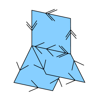
Figure 1: Branching of $SU(3)$ center vortices: The left-hand panel depicts a three-dimensional subspace, where a single vortex line with triality $q=2$ (double arrow) branches into two vortices of triality $q=1$ each (single arrows). The right-hand panel displays a four-dimensional hypercubic lattice view, where vortex surfaces, consisting of elementary squares, branch along links. Elementary squares are associated with curls (see main text), which must cancel on each link (modulo 3) according to the Bianchi identity.

In the four-dimensional picture, one chooses an orientation associated with each elementary square by defining a sense of curl, i.e., a sense in which the links bordering the square are run through, cf. fig. 1. Additionally, each of these curls is endowed with a magnitude, namely the triality $q=1$ or $q=2$ describing the vortex flux carried by the elementary square. Then the Bianchi identity corresponds to a constraint to be satisfied on each lattice link: The sum of the curls attached to the link (with opposite orientation implying opposite sign of the contribution) must vanish modulo 3, as happens on the central link in the right-hand panel of fig. 1. It is not necessary at this point to undertake any effort to cast this condition in formal language; as will become clear below, in practice there will be no need to check the Bianchi constraint for any vortex configurations since the Monte Carlo update procedure generating the vortex world-surface ensemble will be such that the Bianchi identity is guaranteed at every step.

2.2 Center vortex model dynamics

For the case of the gauge group $SU(2)$, an effective model for infrared Yang-Mills dynamics based on center vortex degrees of freedom was presented in [15], where the physical motivation for such random vortex world-surface models is discussed in depth. In addition to the confinement properties studied in [15], the model also turns out to successfully describe the topological properties of $SU(2)$ Yang-Mills theory [21] and the spontaneous breaking of chiral symmetry [24]. The physical principles underlying this vortex model can also be applied to the gauge group $SU(3)$. Adapted to the $SU(3)$ case, they are:

1. Description of vortex world-surfaces: Vortex world-surfaces will be described by composing them of elementary squares on a hypercubic lattice, as already mentioned above. Each elementary square on the hypercubic lattice will be associated with a triality $q_{\mu\nu}(x)\in\{-1,0,1\}$, where $x$ denotes the lattice site from which the elementary square extends into the positive $\mu$ and $\nu$ directions. The ordering of the indices corresponds to the curl already mentioned in the previous section in connection with the Bianchi identity: The value of $q_{\mu\nu}(x)$ specifies the value of the curl corresponding to starting out from $x$ into the positive $\mu$ direction, and then onwards around the elementary square. For definiteness, the indices will usually be ordered such that $\mu<\nu$. If for notational convenience $q_{\nu\mu}(x)$ with $\nu>\mu$ is quoted instead, then this is defined as $q_{\nu\mu}(x)=-q_{\mu\nu}(x)$ in accordance with the remarks in the previous section. The value $q_{\mu\nu}(x)=0$ means that the elementary square is not part of a vortex surface, whereas the values $q_{\mu\nu}(x)=\pm 1$ label the two possible types of vortex flux which may be carried by the elementary square.

   Having thus specified the labeling of the elementary squares making up the vortex surfaces, one can now also give their precise effect on the elementary Wilson loops (plaquettes) $U_{\kappa\lambda}(y)$ they pierce. It should be emphasised once again that Wilson loops are defined on a lattice dual to the one on which the vortex surfaces are constructed. In analogy to the description of vortex elementary squares given above, the elementary Wilson loop $U_{\kappa\lambda}(y)$ thus refers to a plaquette extending from $y$ into the positive $\kappa$ and $\lambda$ directions, with the integration oriented such that one starts at $y$, integrates first into the positive $\kappa$ direction, and then onwards around the plaquette. The plaquette $U_{\kappa\lambda}(y)$ is pierced precisely by the dual lattice elementary square $q_{\mu\nu}(x)$, where the indices $\kappa,\lambda,\mu,\nu$ span all four space-time dimensions and $x=y+(\vec{e}_{\kappa}+\vec{e}_{\lambda}-\vec{e}_{\mu}-\vec{e}_{\nu})a/2$, with $a$ denoting the lattice spacing. $U_{\kappa\lambda}(y)$ can thus be given exclusively in terms of the corresponding $q_{\mu\nu}(x)$, namely

   $$U_{\kappa\lambda}(y)=\exp\left(i\pi/3\cdot\epsilon_{\kappa\lambda\mu\nu}\,q_{\mu\nu}(x)\right)$$ (6)

   (with the usual Euclidean summation convention over Greek indices).

2. Transverse Thickness: In the full Yang-Mills theory, vortices possess a physical thickness perpendicular to the vortex surface, i.e. they are non-singular field configurations with finite action [7, 25]. They resemble Nielsen-Olesen vortices [5] rather than infinitely thin magnetic flux tubes. In particular, this means that vortices cannot be packed arbitrarily densely: If two parallel vortices approach each other closer than the average transverse thickness of their profile, they become undistinguishable from a single vortex with the triality of the two component vortices summed. In the $SU(2)$ model, this means that they annihilate and become equivalent to the vacuum. In the $SU(3)$ case, however, the $Z(3)$ triality algebra, eq. (2), allows e.g. for two $q=1$ vortices to combine into a single $q=2$ vortex if they come sufficiently close.

   In the present vortex model, this behavior is reflected in a fixed, finite physical value of the lattice spacing $a$ which mimics transverse vortex extension: Parallel vortices at a distance smaller than $a$ are not resolved and instead are replaced by a single vortex of the summed triality.

   This should be contrasted with the center projection vortices [7, 9] which can be extracted from lattice gauge configurations on arbitrarily fine lattices. They represent only a rough localisation of physical thick vortices and fluctuate rapidly on all wavelengths even if the underlying thick vortex structure is smooth. In addition, the exact position of a center projection vortex within the thick profile of the physical vortex it is extracted from depends on the details of the gauge fixing procedure [9]. The center projection vortex effective action therefore presumably is very complicated and in particular non-local as the cutoff diverges into the ultraviolet, while a true low energy effective theory should only retain degrees of freedom which fluctuate on wavelengths up to a certain upper limit (provided here by the lattice spacing). In this spirit, the vortices described by the present model, though formally still composed of infinitely thin elementary squares, represent the smooth centers of the profiles of physical (thick) vortices rather than the aforementioned rapidly fluctuating thin projection vortices. Alternatively, one may think of the model vortices treated here as thin center projection vortices with the short distance fluctuations averaged out down to a scale $a$ set by the fixed lattice cutoff. This point of view entails that the vortex action should be well described by a few local terms in the spirit of a derivative expansion [9].

3. Vortex Action: Vortex creation costs a certain action per unit area. This is the first term expected from a derivative expansion [9],

   $$S_{\rm area}[q]=\epsilon\sum_{x}\sum_{\mu,\nu\atop\mu<\nu}\left|q_{\mu\nu}(x)\right|\,,$$ (7)

   where this form of the action assumes that the triality labelings have been chosen such that $q_{\mu\nu}(x)\in\{-1,0,1\}$. Note thus that $S_{\rm area}$ is symmetric with respect to the two possible types of vortex flux.

   Vortices are also stiff, i.e. there is a penalty in the action for bends in the vortex surfaces. To be specific, an action increment $c$ is incurred for each pair of elementary squares in the lattice which share a link and are part of a vortex, but do not lie in the same plane. This can be expressed in terms of a sum over links,

   $$S_{\rm curv}[q]\!\!\!\! = \!\!\!\!c\sum_{x}\sum_{\mu}\Bigg{[}\sum_{\nu<\lambda\atop\nu\neq\mu,\lambda\neq\mu}\Big{(}|q_{\mu\nu}(x)\,q_{\mu\lambda}(x)|+|q_{\mu\nu}(x)\,q_{\mu\lambda}(x-e_{\lambda})|$$

   $$\ \ \ \ \ \ \ \ \ \ \ \ \ \ \ \ \ \ +|q_{\mu\nu}(x-e_{\nu})\,q_{\mu\lambda}(x)|+|q_{\mu\nu}(x-e_{\nu})\,q_{\mu\lambda}(x-e_{\lambda})|\Big{)}\Bigg{]}$$

   $$= \!\!\!\!\frac{c}{2}\sum_{x}\sum_{\mu}\left[\left[\sum_{\nu\neq\mu}\left(|q_{\mu\nu}(x)|+|q_{\mu\nu}(x-e_{\nu})|\right)\right]^{2}\!\!\!-\!\!\sum_{\nu\neq\mu}\!\!\Big{[}|q_{\mu\nu}(x)|+|q_{\mu\nu}(x-e_{\nu})|\Big{]}^{2}\ \right]\ .$$

   As in the case of $S_{\rm area}$, these expressions for $S_{\rm curv}$ assume that the triality labelings have been chosen such that $q_{\mu\nu}(x)\in\{-1,0,1\}$. Also $S_{\rm curv}$ is symmetric with respect to the two possible types of vortex flux.

   This is a plausible model assumption in view of the fact, already discussed further above, that the two types of vortex flux are related by a space-time inversion, at least as far as their effect on Wilson loops is concerned. Nevertheless, it should be noted that the curvature action presented above is not the most general one which involves elementary squares sharing a link and which respects the aforementioned symmetry. The form (3) manifestly is a sum of terms depending only on pairs of elementary squares attached to a given link; there are no higher order terms simultaneously involving more than two elementary squares such as $|q_{\mu\nu}(x)q_{\mu\lambda}(x)q_{\mu\kappa}(x)|$, which would be entirely admissible. This type of truncation was already assumed in the $SU(2)$ case [15]; it does not constitute a new feature of the present investigation and serves to keep the number of independent coupling constants small and the model predictive.

4. Monte Carlo update procedure and continuity of flux: The model vortex dynamics will be realized by generating an ensemble of random vortex world-surfaces using a Monte Carlo procedure weighted with the action presented above. The elementary update will be chosen such that continuity of flux is guaranteed at every step. Namely, choose an elementary three-dimensional cube in the lattice extending from a lattice site $x$ into the positive $\mu$, $\nu$ and $\lambda$ directions. Update the configuration by adding the flux corresponding to a vortex shaped as the elementary cube surface to the flux previously present. All six elementary squares making up the surface of the cube are thus updated simultaneously as follows,

   $$\begin{array}[]{l@{\qquad}l}q_{\mu\nu}(x)\to q_{\mu\nu}(x)+w\,,&q_{\mu\nu}(x+e_{\lambda})\to q_{\mu\nu}(x+e_{\lambda})-w\\ q_{\nu\lambda}(x)\to q_{\nu\lambda}(x)+w\,,&q_{\nu\lambda}(x+e_{\mu})\to q_{\nu\lambda}(x+e_{\mu})-w\\ q_{\lambda\mu}(x)\to q_{\lambda\mu}(x)+w\,,&q_{\lambda\mu}(x+e_{\nu})\to q_{\lambda\mu}(x+e_{\nu})-w\end{array}$$ (9)

   with $w=\pm 1$ . In practice, the value $w$ with which the update is attempted (i.e. the triality of the superimposed cubic vortex) is chosen at random with equal probability. Since the linear superposition of two configurations which satisfy continuity of flux leads again to a configuration which satisfies that constraint, the update algorithm preserves Bianchi’s identity, eq. (5), at every step while allowing to generate every valid vortex world-surface configuration.

\psfrag{xx}{$\epsilon$}\psfrag{yyy}{$c$}\psfrag{zzzzzz}{$\sigma_{0}\,a^{2}$}\includegraphics[width=227.62204pt]{all.eps} \psfrag{eeeee}{$\epsilon$}\psfrag{ccccccc}{$c$}\includegraphics[width=199.16928pt]{constant.eps}

Figure 2: Plane of coupling constants $(\epsilon,c)$. The left-hand panel shows the zero-temperature string tension $\sigma_{0}$ in units of the lattice spacing, as a function of $\epsilon$ and $c$. In the right-hand panel, the three-dimensional representation has been replaced by a density plot in which brighter colours indicate higher string tension. The thick white line in the confining region locates pairs $(\epsilon,c)$ at which the ratio $T_{c}/\sqrt{\sigma_{0}}\approx 0.63$ of full $SU(3)$ Yang-Mills theory is reproduced.

3 Confinement properties and the space of coupling constants

The model described in the previous section formally has three independent parameters, namely, the two dimensionless coupling constants $\epsilon$ and $c$ introduced in the action, and the dimensionful lattice spacing $a$. As emphasised above, the spacing $a$ has a definite physical interpretation and thus must be given a fixed physical value rather than being taken to zero as in conventional lattice gauge theories. Eventually, $a$ will be fixed by fitting the zero-temperature string tension $\sigma_{0}$ to the phenomenological value

$$\sigma_{0}=(440\,\mathrm{MeV})^{2}\,.$$ (10)

With this arrangement, the lattice spacing $a$ is assigned a physical value which determines the transverse thickness of the vortices (see previous section). Moreover, it provides the ultraviolet cutoff for the largest momenta $|p|=\pi/a$ which can be resolved in this low energy effective theory, and it sets the scale for all dimensionful quantities.

With the determination of $a$ understood, consider the phase diagram of the model in the coupling constant ($\epsilon,c$) space. Figure 2 shows the result of Wilson loop measurements on a symmetric $16^{4}$ lattice, which represents the zero-temperature approximation. From the Wilson loops, the string tension $\sigma_{0}$ can be extracted e.g. by computing Creutz ratios or directly by fitting the area-law fall-off. The result is a simple phase diagram containing a confining and a non-confining region, cf. the left-hand panel of fig. 2. The confining region is located at small $c$ and small or even negative $\epsilon$, where the formation of a high density of connected, crumpled vortex world-surfaces is favoured.

For a large range of coupling constants, one furthermore encounters a deconfinement transition to a phase with vanishing string tension when raising the temperature by decreasing the number of lattice spacings $N_{0}$ in the Euclidean time direction. At finite temperatures, the heavy quark potential must be extracted from Polyakov loop correlators. Since the model is Abelian, this is equivalent to measuring time-like $(N_{0}\times R)$ Wilson loops with maximal extension in the Euclidean time direction.

As emphasised above, the lattice spacing of the model is a fixed quantity that cannot be adjusted towards a continuum limit. As a consequence, changing $N_{0}$ while keeping $(\epsilon,c)$ fixed only allows to alter the temperature in rather big steps. To obtain additional data, an interpolation method [15] is used: For fixed $\epsilon$, $N_{0}=1,2,3$ are considered in turn and $c$ is varied until the deconfining phase transition is observed at a critical coupling $c^{\ast}(N_{0})$. This in turn yields the critical temperature $aT_{c}=1/N_{0}$ for the pair $(\epsilon,c^{\ast}(N_{0}))$, from which $aT_{c}(\epsilon,c)$ may be obtained for all couplings by interpolation.

With measurements, in lattice units, of the critical temperature, $aT_{c}$, and the zero-temperature string tension, $\sigma_{0}a^{2}$, the physical ratio $T_{c}/\sqrt{\sigma_{0}}$ can be computed for all values of the coupling constants $\epsilon,c$. Measurements in full $SU(3)$ lattice Yang-Mills theory favour the value $T_{c}/\sqrt{\sigma_{0}}\approx 0.63$ for the gauge group $SU(3)$ [26]. Taking this number as a second input (besides the value eq. (10) of the string tension) yields the white line in the right-hand panel of fig. 2. Note that points of the same colour in that plot indicate the same string tension in lattice units $\sigma_{0}a^{2}$, i.e. $\sigma_{0}a^{2}$ does not vary considerably on the white physical line. As $\sigma_{0}$ is being used to fix the lattice spacing, this entails in turn that the spacing itself will be approximately constant along the physical line (it varies only by about 10 %).

On the one hand, this corroborates the physical picture of the lattice spacing as a fixed quantity determining the spatial resolution and the transverse thickness of the vortices. Further measurements, such as of the spatial string tension, provide additional evidence that physics is approximately constant along the white line in fig. 2. This means that one cannot use further physical input to find the unique point in the phase diagram where the model matches low-energy Yang-Mills theory: There is an entire line of such points which, to a good approximation, are equivalent. This is discussed in more detail in [15] for the $SU(2)$ case, where the same phenomenon occurs. For convenience, one specific point on the physical trajectory will be chosen in the following and all measurements will be performed with the parameters

$$\epsilon=0\,,\qquad\qquad c=0.21$$ (11)

unless stated otherwise. For this choice of parameters, the lattice spacing as extracted from eq. (10) is

$$a=0.39\,\mathrm{fm}\,,$$ (12)

which equals the spacing found in the $SU(2)$ model [15]. For other points on the physical trajectory, the lattice spacing deviates less than 10 % from this value, with lower $\epsilon$ giving slightly smaller $a$.

Having chosen a physical set of parameters, one can begin to predict further quantities. Fig. 3 displays measurements of the string tension between static colour sources as well as the spatial string tension as a function of temperature. While the deconfinement temperature reflected in the string tension between static colour sources has been used in fixing the coupling constants, the behavior of the spatial string tension, extracted from spatial Wilson loops, does not enter the construction of the model and is thus predicted. Particularly the behavior at high temperatures, where a finite spatial string tension persists, is interesting. In the $SU(2)$ case [15], the obtained model values agreed with the ones measured in $SU(2)$ lattice Yang-Mills theory to within 1%; such high agreement certainly is coincidental in view of the fact that those measurements take place near the ultraviolet limit of validity of the vortex model. In the $SU(3)$ case, cf. fig. 3, the agreement at the highest temperature, $T=1.80\,T_{c}$, is still impressive, namely to within 5% compared with the full $SU(3)$ Yang-Mills value obtained in [26]. This is furthermore well within the error bars quoted in [26].

Figure 3: String tension between two static colour charges (crosses) and spatial string tension (squares) as a function of temperature. Measurements were taken on a $16^{3}\times N_{0}$ lattice for the physical choice of parameters, eq. (11). The error bar for the temporal string tension at $T/T_{c}=0.90$ reflects a systematic uncertainty resulting from subleading logarithmic corrections in the potential near the phase transition [27].

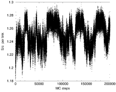
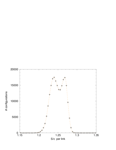
Figure 4: Left-hand panel: Action per link as a function of the Monte Carlo simulation time. Measurements were taken on a $30^{3}\times 2$ lattice at the deconfinement phase transition point $\epsilon=0$ and $c=0.2359$. This set of parameters is close to the physical trajectory, cf. main text. The right-hand panel shows the same data as a histogram of configurations binned according to their curvature action. The resulting action distribution exhibits the double peak structure characteristic for a first order phase transition.

4 Finite temperature phase transition

A topic of particular interest is the order of the deconfining phase transition. Ideally, one would be interested in studying the physical point $c=0.21$, $\epsilon=0$ and directly varying the temperature via the temporal extension of space-time. In practice, only discrete values of the temporal extension are accessible directly at $c=0.21$; for this reason, the authors instead worked at a fixed number of temporal lattice spacings $N_{0}=2$ and varied $c$ around the phase transition point, which is located at $c=0.2359$ (on $30^{3}\times 2$ lattices). This is rather close to the physical value $c=0.21$ and thus is expected to furnish a good indication of physics there. Note that results directly on the physical trajectory could be obtained using an interpolation procedure [15] based on studying the phase transition at several $N_{0}$ and the associated critical values $c^{*}(N_{0})$; however, such an interpolation would indeed be dominated by the results at $N_{0}=2$, $c=0.2359$ given below. The above accurate estimate of the critical value, $c=0.2359$, was determined by finding the maximal slope of the curvature action per lattice link as a function of $c$. Subsequently, the authors carried out long Monte Carlo runs on large, $30^{3}\times 2$ lattices, recording the curvature action per lattice link for every configuration. Such a Monte Carlo history is depicted in fig. 4. It displays the behavior characteristic of a first order phase transition, as is to be expected for a model with $Z(3)$ symmetry [28]. As the Monte Carlo process progresses, the value of the action per lattice link at times fluctuates around a lower mean value (deconfined phase) and at other times around an upper mean value (confined phase). At $c=0.2359$, the two cases occur with approximately equal weight. At the neighboring value $c=0.2357$, the effect of the phase transition is still easily discernible, whereas at $c=0.2361$, the evidence is already rather tenuous, cf. fig. 5.

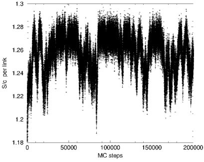
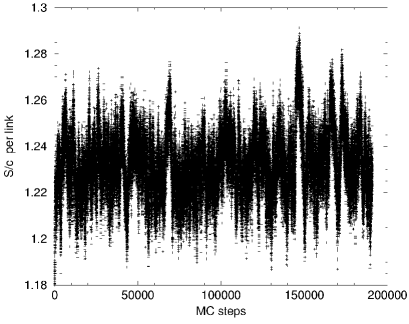
Figure 5: Action per link as a function of Monte Carlo time. Measurements were taken on a $30^{3}\times 2$ lattice with $\epsilon=0$. The value of the curvature coupling $c$ was chosen such that the system is biased slightly towards the confined phase (left-hand panel, $c=0.2357$) and the deconfined phase (right-hand panel, $c=0.2361$), respectively.

It is important to note the rather weak first-order behavior. The difference between the aforementioned mean values in the two phases is small and it was necessary to go to very large, $(30a)^{3}$ spatial universes to sufficiently suppress the fluctuations around each of the mean values such as to be able to distinguish the two phases. On such large lattices, one indeed observes the characteristic double-peak structure in a histogram of the action per lattice link at $c=0.2359$, cf. the right-hand panel of fig. 4. On smaller lattices, the fluctuations in each individual phase swamp the difference in the mean action per lattice link between the phases and the double-peak structure cannot be resolved. It should be noted that the weakness of the transition obtained near the physical point is a nontrivial prediction of the model; in fact, at other, nonphysical points in the plane of coupling constants, one can observe very strongly first order phase transition behaviour, cf. fig. 6. This figure was obtained at $c=0,\epsilon=0.993$ on very small, $4^{3}\times 2$ lattices. Even then, the very large difference in the action density between the two phases is clearly visible. Note that this case (with no curvature action, $c=0$) corresponds to (the dual formulation of) standard $Z(3)$ lattice gauge theory.

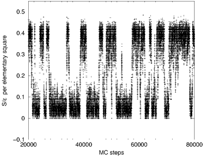
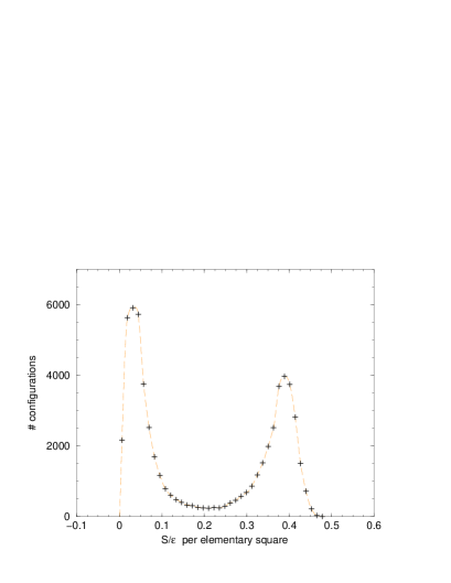
Figure 6: Left-hand panel: Action per elementary square as a function of Monte Carlo time at the (unphysical) point $c=0$ and $\epsilon=0.993$. The corresponding action distribution in the right-hand panel exhibits a clear signal of a strong first order phase transition for this unphysical choice of parameters, even on very small lattices (measurements were taken on a $4^{3}\times 2$ lattice).

The weakness of the transition observed near the physical point in figs. 4 and 5 matches the result in full $SU(3)$ Yang-Mills theory, where the first order character of the deconfining phase transition also turns out to be rather weak [29]. This constitutes a successful nontrivial test of the correspondence between $SU(3)$ Yang-Mills theory and the present random vortex world-surface model.

To complete the discussion of the order of the deconfining phase transition in the vortex model, the authors also revisited the $SU(2)$ case, in which the transition is expected to be second order. This topic was not studied in detail in [15]. As above, $30^{3}\times 2$ lattices were used and the value of $c$ at which the phase transition occurs was localized in the interval $0.298<c<0.300$ by looking for the maximal slope in the curvature action per lattice link. Taking the $SU(3)$ case as an indication, where the first order character of the phase transition was discernible over a range of $c$ of width larger than $0.0002$, cf. figs. 4 and 5, the authors scanned the region $c=0.296$ to $c=0.302$ in steps of $0.0002$ and recorded Monte Carlo histories analogous to figs. 4 and 5. None of them displayed a significant indication of a first order phase transition (cf. fig. 7 as an example; the other Monte Carlo histories were of the same qualitative character). Thus, at least to the accuracy which proved sufficient to ascertain the order of the transition in the $SU(3)$ case, the $SU(2)$ model appears to behave in a manner which is consistent with $SU(2)$ lattice Yang-Mills theory and which is expected from Ginzburg-Landau analysis [28], i.e., it appears to display a second-order deconfinement phase transition. Of course, the data do not exclude a first order transition of considerably weaker character than in the $SU(3)$ case. The authors did carry out a more detailed finite-size analysis using lattices of varying spatial extension.

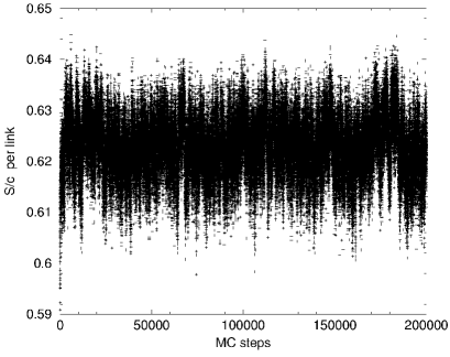
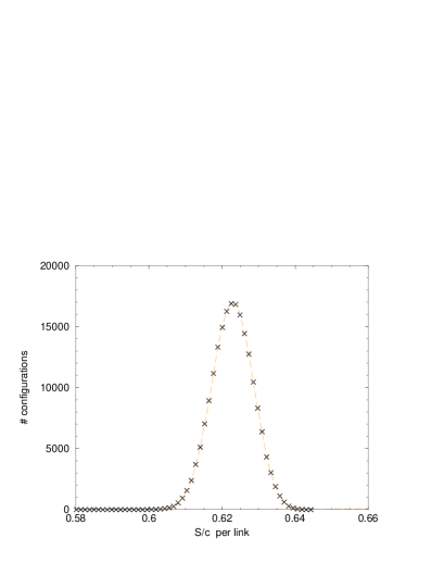
Figure 7: Left-hand panel: Action per link as a function of Monte Carlo time in the region of the deconfining phase transition for the $SU(2)$ vortex model studied in [15]. Measurements were taken on a $30^{3}\times 2$ lattice with $\epsilon=0$ and $c=0.2990$. This data should be compared to the $SU(3)$ case depicted in fig. 4. At least to the accuracy which was sufficient to detect a double peak structure in the $SU(3)$ action distribution, the $SU(2)$ model exhibits the characteristics of a second order transition, as shown by the single peak structure of the $SU(2)$ action distribution displayed in the right-hand panel.

5 The structure of vortex clusters

The confinement properties of the model are intimately tied to the percolation properties of the vortices. In the $SU(2)$ case studied in ref. [15], a percolation transition at finite temperatures, inducing deconfinement, became apparent. This analysis can be analogously extended to the present $SU(3)$ version of the model. Since the findings are very similar to the aforementioned $SU(2)$ case, this section will be kept rather brief. For a detailed exposition of the connection between vortex percolation and confinement, the reader is referred to [15].

In order to exhibit the percolation properties of vortices, it is useful to consider three-dimensional slices of space-time, taken between vortex lattice (hyper-)planes, keeping either one space coordinate or the time coordinate fixed. Since this situation will appear frequently in the following, such three-dimensional slices will be referred to as space and time slices, respectively.

In any such three-dimensional slice, vortices form closed loops made up of links which, in general, will self-intersect to form complicated vortex clusters. A cluster is defined as a (maximal) set of connected vortex links and its extension as the maximal Euclidean distance between any two links in that cluster. Fig. 8 shows the probability distribution for vortex links to belong to a cluster of a given extension. These measurements were taken in space slices and exhibit a clear signal of a percolation transition: Below $T_{c}$, most vortex links are in clusters of nearly maximal extension, while the deconfined region above $T_{c}$ is dominated by many small clusters which do not percolate. Note that the persistence of clusters of maximal extension slightly above the deconfinement temperature (cf. center panel in the lower line of fig. 8) is natural. At temperatures so close to the phase transition, one must expect a significant density of clusters which are as large as the lattice universe used, and which would only be revealed as non-percolating in significantly larger lattice universes. To verify this, a detailed finite-size analysis using lattices of different extensions is necessary. In complete correspondence, of course, the deconfinement temperature itself is only defined up to finite-size effects.

The above picture changes drastically if one considers time slices instead of space slices. Here, vortex lines percolate in both phases. This is seen in the probability distribution of vortex cluster extensions in time slices. To compare with the previous results in fig. 8, one now has to normalise to the maximal possible extension in time slices, i.e. $\sqrt{3}N_{s}a/2$. As can be seen from fig. 9, the distributions show no sign of a phase transition and remain strongly peaked at the maximal extension for all temperatures. This means that virtually all vortex links in time slices belong to clusters of maximal spatial extension; the clusters percolate for all temperatures.

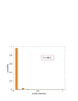
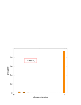
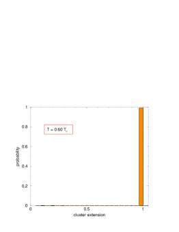
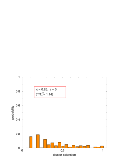
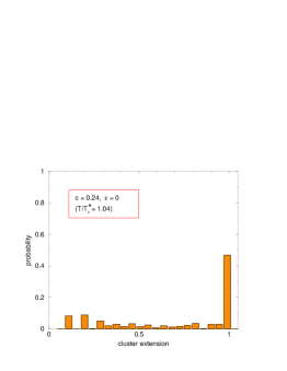
Figure 8: Probability distributions obtained by binning vortex links belonging to space slices of the random vortex surfaces according to the extension of the vortex cluster they belong to. Cluster extensions are measured in units of the maximal possible extension, see main text. The top line shows measurements taken using $16^{3}\times N_{0}$ lattices at the physical point (11), both in the confined and the deconfined phase. Since these graphs do not give a detailed picture of the behaviour close to the phase transition itself, the lower line presents cluster distributions taken on a $16^{3}\times 2$ lattice with $\epsilon=0$ and $c=0.26,\,0.24,\,0.23$ (from left to right). While these points correspond formally to $T/T_{c}^{\ast}=1.14,\,1.04\,,0.99$, they do not lie on the physical trajectory. As a consequence, the transition temperature $T_{c}^{\ast}$ at these points (as obtained by the interpolation procedure described in section 3) is not identical to the physical $T_{c}$, but rather a formal quantity which is undetermined in absolute units. As already explained for the Monte Carlo histories in the previous section, the parameters are still sufficiently close to the physical trajectory to provide an accurate indication of physics there.

A more detailed picture of the deconfined phase emerges from the study of the number of links contained in the clusters. For the set of parameters (11), only $N_{0}=1$ realises the deconfined phase. In space slices of this lattice, $96.5$% of all vortex links are contained in clusters with only one link (those links are the entire cluster and wind directly around the Euclidean time direction). At $N_{0}=2$, which is below $T_{c}$, the fraction of vortex links belonging to winding clusters consisting of two links is only about $2.9$%, while most vortex flux is contained in clusters of roughly $500$ links. For time slices, on the other hand, there is no significant difference between $N_{0}=1$ and $N_{0}=2$: The majority of vortex links in both cases is contained in clusters made up of more than $4000$ links. Thus, the small vortex clusters which dominate the deconfined phase in space slices are mainly winding vortex configurations which run directly along the compactified time direction.

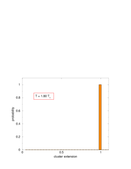
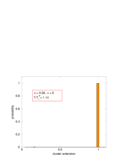
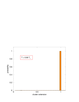
Figure 9: Probability distributions obtained by binning vortex links belonging to time slices of the random vortex surfaces according to the extension of the vortex cluster they belong to. Cluster extensions are measured in units of the maximal possible extension, see main text. While the left and right-hand histograms were obtained using $16^{3}\times N_{0}$ lattices at the physical point $(c=0.21,\epsilon=0)$, the graph in the middle results when using a $16^{3}\times 2$ lattice at the point $(c=0.26,\epsilon=0)$, which does not lie on the physical trajectory. In analogy to the discussion in the caption of fig. 8, the label $T/T_{c}^{\ast}=1.14$ indicates that the measurement is performed slightly above the phase transition temperature, but the ”local” $T_{c}^{\ast}$ at an unphysical point on the plane of coupling constants is a formal quantity and not identical to the physical $T_{c}=277$ MeV in the left and right-hand panels.

The situation is different at (unphysical) points in coupling constant space where deconfinement is observed even at zero temperature. In this case, there is of course no finite temperature phase transition and analogous measurements show that no percolating vortex clusters exist in either time or space slices, at all temperatures. All these findings are virtually identical to the corresponding results obtained for the $SU(2)$ case in [15]. To summarise, this confirms that also in the $SU(3)$ case, confinement is generated by percolating vortex clusters while the deconfined phase is characterised (in space slices) by small disconnected clusters which predominantly wind around the (short) Euclidean time direction of the lattice universe. For a more detailed physical discussion of the connection between vortex percolation and confinement, the reader is referred to [15].

6 Vortex branching

The model action, eqs. (7) and (3), presented in section 2 is essentially equivalent to the $SU(2)$ case [15]. It does not contain terms that enhance or penalise vortex branchings explicitly. Nonetheless, the finite temperature studies in section 4 indicate that the larger phase space of $SU(3)$ vortices, i.e. the possibility of vortex branchings, can make a physical difference to the $SU(2)$ case: It changes the order of the deconfinement phase transition. It is therefore interesting to study the distribution of vortex branchings in the Monte Carlo ensembles in more detail.

To do so, it is useful to consider three-dimensional slices of space-time as in the previous section. Vortices branch along lines (links) in four dimensions, so taking a three-dimensional slice yields a three-dimensional distribution of branching points. Just as any given link in four dimensions is attached to six elementary squares (which may or may not be part of a vortex), each site in the three-dimensional slice can be attached to up to six vortex links. As explained in section 2, the model description does not keep track of vortex orientation and cannot distinguish between, say, a $z_{2}$-vortex branching into two $z_{1}$-vortices, or three $z_{1}$-vortices annihilating along a common link in four dimensions. In fact, corresponding to the symmetry of the underlying action with respect to the two possible types of vortex flux, the only measurable physical quantity is the number $\nu$ of vortex surfaces meeting at each link,

• $\nu=0$ indicates that the link is not part of any vortex

• $\nu=1$ is forbidden, since vortices are closed and there are no end links (Bianchi’s identity)

• $\nu=2$ indicates that the link is part of a vortex surface which does not branch or self-intersect at that link

• $\nu=4,6$ represent vortex self-intersections already present in the $SU(2)$ case

• $\nu=3,5$ indicate true $SU(3)$ vortex branchings which have no counterpart in $SU(2)$

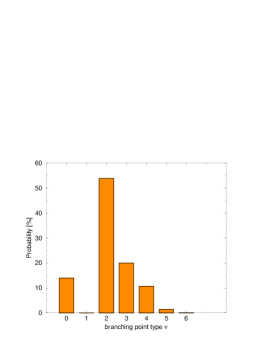
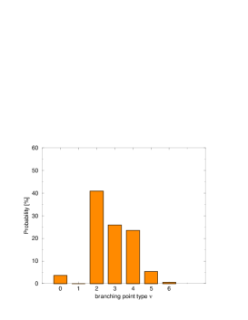
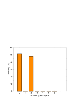
Figure 10: Distribution of branching points in three-dimensional slices of space-time, all measured at the physical point $\epsilon=0$ and $c=0.21$. The left-hand panel shows the results obtained using a symmetric $16^{4}$ lattice (i.e. at zero temperature) while the center and right-hand panels give the distributions obtained using a $16^{3}\times 1$ lattice (i.e. in the deconfined phase). The graph in the middle refers to a time slice while the right-hand panel shows the corresponding result for a space slice.

An example of a branching with $\nu=3$ is displayed in fig. 1. Figure 10 shows the result of measurements of the $\nu$ distribution in three-dimensional slices of space-time at the physical point, eq. (11). In all cases, there are indeed no vortex end points, $\nu=1$, as vortices are constrained to be closed. For the symmetric $16^{4}$ lattice used to obtain the left-hand panel, the majority of points is associated with $\nu=2$, i.e. they represent sites where the vortex does not branch. However, vortex branchings $\nu=3,5$ as well as self-intersections $\nu=4,6$ occur with a significant probability, indicating that the structure of vortices is quite fibrated in this case. Note that a sufficiently large symmetric lattice is approximately at $T=0$, which is in the confining phase for the parameters eq. (11).

The two other panels of fig. 10 show the branching point distribution for the same parameters, eq. (11), but now at high temperatures (on an asymmetric $16^{3}\times 1$ lattice) where the model is in the deconfined phase. For time slices (center panel), there is no qualitative change as the probability of branchings even increases slightly. This indicates that vortex fibration is significant along temporal links and the structure of vortex clusters in time slices does not change qualitatively across the phase transition. This result is in line with the earlier finding that vortex percolation persists in time slices in the deconfined phase.

In space slices (cf. right-hand panel of fig. 10), the vortex structure changes strongly as one increases the temperature into the deconfined regime. Branching points and self-intersections are strongly suppressed, even though vortices still abound; almost half of the lattice sites in a three-dimensional space slice are still located on vortices. This is consistent with the fact that the vortices are to a large extent aligned along the short Euclidean time direction; branchings, which would imply vortices splitting off into spatial directions, are correspondingly rare. In a space slice, the complicated, fibrated vortex cluster of the confining phase has turned into small, mostly non-fibrated vortices which are not interconnected and cease to percolate. It should be noted that the fraction of lattice sites in the three-dimensional space slice with $\nu\neq 0$ drops only moderately across the phase transition – from $85\%$ in the confining phase to $50\%$ in the deconfined phase. Thus, it is really the change in vortex structure engendered by the percolation transition, not the overall vortex density, which drives the deconfining phase transition.

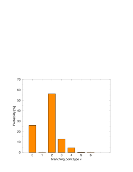
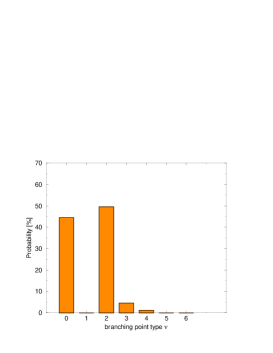
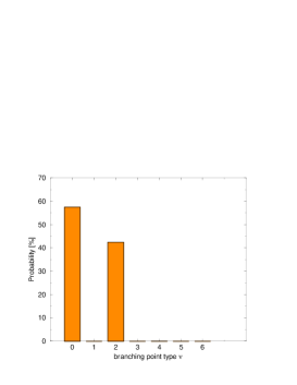
Figure 11: Distribution of branching points in three-dimensional space slices obtained at the (unphysical) point $\epsilon=0$ and $c=0.30$. The measurements were taken on an asymmetric $16^{3}\times N_{0}$ lattice, with $N_{0}=3,2,1$ (from left to right), i.e. the temperature increases from left to right. The distribution at $N_{0}=3$ (left) is virtually identical to the zero-temperature (confining) case $N_{0}=16$, while $N_{0}=2$ (center) and $N_{0}=1$ (right) are in the deconfined phase.

For the physical point $\epsilon=0$, $c=0.21$, it is necessary to let the Euclidean time extension of the lattice universe shrink to $N_{0}=1$ in order to observe the deconfined phase. This case is, however, somewhat special, since then, vortices extending in the time direction necessarily close via the periodic boundary conditions, i.e. they automatically wind around the Euclidean time dimension. To corroborate that the suppression of branching points in the deconfined phase is not an artefact of $N_{0}=1$, the authors have furthermore investigated the (unphysical) point $\epsilon=0$, $c=0.30$, where $N_{0}=2$ is also well within that phase. Fig. 11 shows data measured on $16^{3}\times N_{0}$ lattices, for various values of $N_{0}$, i.e. various temperatures. The change in vortex structure discussed above, i.e., the suppression of branchings, now also becomes apparent in the $N_{0}=2$ case, although it should be noted that the branching density evidently does not behave as a strict order parameter; while strongly suppressed, the probability of branchings displayed in the center panel of fig. 11 is not entirely negligible.

Similar results are also seen as one traverses the crossover in fig. 2 by varying the coupling constants $\epsilon$ and $c$. Figure 12 presents the distribution of branching points in three-dimensional slices of space-time measured using a symmetric $16^{4}$ lattice, both at the point $\epsilon=0.25$, $c=0.3$ in the deconfined region (left-hand panel) and at $\epsilon=-0.2$, $c=0.1$ in the confining region (right-hand panel). While branching points are abundant in the confining region (indicating the existence of heavily fibrated vortex clusters in this case), they are virtually absent in the deconfined region. Since there are no short directions on a $16^{4}$ lattice for vortices to wind around, the absence of branching points for the deconfining parameters in this case is due to space-time being filled with small vortex structures which are disconnected and do not percolate in any direction.

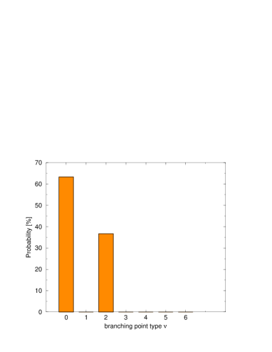
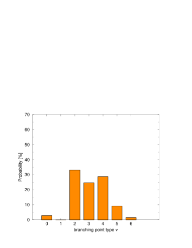
Figure 12: Distribution of branching points in three-dimensional slices of space-time measured using a $16^{4}$ lattice at the points $\epsilon=0.25$, $c=0.3$ (deconfined region, left-hand panel) and $\epsilon=-0.2$, $c=0.1$ (confining region, right-hand panel).

7 Conclusions and outlook

In the present work, the random vortex world-surface model for the infrared sector of Yang-Mills theory, previously developed for the gauge group $SU(2)$ [15], was extended to the gauge group $SU(3)$. As in the $SU(2)$ case, it proved possible to quantitatively reproduce the confinement properties of the corresponding lattice Yang-Mills theory. Both the low-temperature confining phase as well as the high-temperature deconfined phase are encompassed by the model, and its coupling constants can be chosen such that the ratio $T_{c}/\sqrt{\sigma_{0}}\approx 0.63$ of full Yang-Mills theory is recovered.

Having fixed the parameters of the model, an accurate prediction of the spatial string tension in the deconfined phase is obtained, as in the $SU(2)$ case. Furthermore, the deconfinement phase transition is predicted to be weakly first order, in agreement with $SU(3)$ lattice gauge theory.

The confinement properties of the model are intimately tied to the percolation properties of the vortices. As in the $SU(2)$ case, confinement is generated when vortices in space slices of the lattice universe (i.e., keeping one spatial coordinate fixed) percolate; by contrast, the deconfined phase is characterized by small, mutually disconnected vortices which are predominantly aligned with the short Euclidean time direction of the space slice and are closed by virtue of the periodic boundary conditions. Nevertheless, there is one important difference in geometry between the $SU(2)$ and $SU(3)$ cases: In the latter case, there are two distinct types of quantized vortex flux and, as a consequence, vortices can branch. This does not happen for $SU(2)$ vortices. In particular, when traversing the finite-temperature phase transition into the deconfined phase, vortex branchings observed in space slices of the lattice universe become strongly suppressed, consistent with the aforementioned alignment of the vortices with the Euclidean time direction in that phase. Note that a significant presence of branchings is only possible when there is no single predominant direction of vortex flux. It is tempting to ascribe the first-order character of the phase transition to this additional qualitative difference between the configurations in the confined and deconfined phases (branching vs. non-branching in space slices); on the other hand, since the branching probability does not strictly behave as an order parameter, this surmise must be treated with caution. A still more detailed understanding of the dynamics at the deconfinement phase transition would be desirable. In the $SU(2)$ case, where no vortex branching can occur, the transition is second order, at least to the level of accuracy which was sufficient to ascertain the first order character in the $SU(3)$ case.

As far as the confinement properties are concerned, an interesting extension of the present model would lie in the treatment of a higher number of colours. In particular, it would be interesting to study whether the deconfinement phase transition becomes more strongly first order, as it does in full lattice Yang-Mills theory [30]. Also, it has recently been argued [31] that a description of the infrared sector of Yang-Mills theory in terms of vortex world-surfaces of a well-defined, finite thickness which percolate throughout space-time may become less appropriate as the number of colours $N_{c}$ increases. It would be interesting to investigate whether, and at what $N_{c}$, signals of this can be detected. At least in terms of the confinement properties of $SU(3)$ Yang-Mills theory studied in the present work, the random vortex world-surface model still seems to perform well.

A further, phenomenologically important point of study concerns the baryonic potential, specifically whether it satisfies an area law of the $\Delta$ type or of the Y type [32, 33]. This is currently being investigated. Moreover, apart from the confinement properties, also the topological properties of the $SU(3)$ random vortex world-surface model, which enter the axial $U_{A}(1)$ anomaly, need to be considered in analogy to the $SU(2)$ case [21]. Finally, to arrive at a comprehensive description of $SU(3)$ infrared strong interaction physics, the coupling to quark fields and the concomitant generation of a chiral condensate must be investigated (cf. ref. [24] for the $SU(2)$ model).

References

- [1] G. ’t Hooft, Nucl. Phys. B138 (1978) 1.
-
[2]
G. Mack and V. B. Petkova, Ann. Phys. (NY) 123 (1979) 442;
G. Mack, Phys. Rev. Lett. 45 (1980) 1378;
G. Mack and V. B. Petkova, Ann. Phys. (NY) 125 (1980) 117;
G. Mack, in: Recent Developments in Gauge Theories, eds. G. ’t Hooft et al. (Plenum, New York, 1980);
G. Mack and E. Pietarinen, Nucl. Phys. B205 [FS5] (1982) 141. - [3] Y. Aharonov, A. Casher and S. Yankielowicz, Nucl. Phys. B146 (1978) 256.
- [4] J. M. Cornwall, Nucl. Phys. B157 (1979) 392.
-
[5]
H.B. Nielsen and P. Olesen, Nucl. Phys. B160 (1979) 380;
J. Ambjørn and P. Olesen, Nucl. Phys. B170 (1980) 60, 265. -
[6]
E. T. Tomboulis, Phys. Rev. D 23 (1981) 2371;
E. T. Tomboulis, Phys. Lett. B303 (1993) 103;
T. G. Kovács and E. T. Tomboulis, Phys. Rev. D 57 (1998) 4054. -
[7]
L. Del Debbio, M. Faber, J. Greensite and Š. Olejník,
Phys. Rev. D 55 (1997) 2298;
L. Del Debbio, M. Faber, J. Giedt, J. Greensite and Š. Olejník, Phys. Rev. D 58 (1998) 094501. -
[8]
C. Alexandrou, M. D’Elia and P. de Forcrand,
Nucl. Phys. Proc. Suppl. 83 (2000) 437;
C. Alexandrou, P. de Forcrand and M. D’Elia, Nucl. Phys. A663 (2000) 1031. - [9] M. Engelhardt and H. Reinhardt, Nucl. Phys. B567 (2000) 249.
- [10] K. Langfeld, H. Reinhardt, O. Tennert, Phys. Lett. B419 (1998) 317.
-
[11]
V. G. Bornyakov, D. A. Komarov and M. I. Polikarpov,
Phys. Lett. B497 (2001) 151;
V. G. Bornyakov, D. A. Komarov, M. I. Polikarpov and A. I. Veselov, JETP Lett. 71 (2000) 231;
R. Bertle, M. Faber, J. Greensite and Š. Olejník, JHEP 0010 (2000) 007;
M. Faber, J. Greensite and Š. Olejník, Phys. Rev. D 64 (2001) 034511;
M. Faber, J. Greensite and Š. Olejník, Nucl. Phys. Proc. Suppl. 106 (2002) 652. -
[12]
K. Langfeld, O. Tennert, M. Engelhardt and H. Reinhardt,
Phys. Lett. B452 (1999) 301;
M. Engelhardt, K. Langfeld, H. Reinhardt and O. Tennert, Phys. Rev. D 61 (2000) 054504. - [13] J. Greensite, Prog. Part. Nucl. Phys. 51 (2003) 1.
- [14] M. Faber, J. Greensite and Š. Olejník, Phys. Lett. B474 (2000) 177.
- [15] M. Engelhardt and H. Reinhardt, Nucl. Phys. B585 (2000) 591.
- [16] P. de Forcrand and M. Pepe, Nucl. Phys. B598 (2001) 557.
- [17] K. Langfeld, hep-lat/0307030.
- [18] H. Reinhardt, Nucl. Phys. B628 (2002) 133.
- [19] J. M. Cornwall, Phys. Rev. D 65 (2002) 085045.
- [20] F. Bruckmann and M. Engelhardt, hep-th/0307219.
- [21] M. Engelhardt, Nucl. Phys. B585 (2000) 614.
- [22] P. de Forcrand and M. D’Elia, Phys. Rev. Lett. 82 (1999) 4582.
- [23] R. Bertle, M. Engelhardt and M. Faber, Phys. Rev. D 64 (2001) 074504.
- [24] M. Engelhardt, Nucl. Phys. B638 (2002) 81.
-
[25]
M. Faber, J. Greensite and Š. Olejník,
Phys. Rev. D 57 (1998) 2603;
M. Faber, J. Greensite and Š. Olejník, Acta Phys. Slov. 49 (1999) 177. - [26] G. Boyd, J. Engels, F. Karsch, E. Laermann, C. Legeland, M. Lütgemeier and B. Petersson, Nucl. Phys. B469 (1996) 419.
- [27] O. Kaczmarek, F. Karsch, E. Laermann and M. Lütgemeier, Phys. Rev. D 62 (2000) 034021.
- [28] B. Svetitsky, Phys. Rep. 132 (1986) 1.
- [29] N. A. Alves, B. A. Berg and S. Sanielevici, Nucl. Phys. B376 (1992) 218.
- [30] B. Lucini, M. Teper and U. Wenger, Phys. Lett. B545 (2002) 197.
- [31] J. Greensite and Š. Olejník, JHEP 0209 (2002) 039.
-
[32]
J. M. Cornwall, Phys. Rev. D 54 (1996) 6527;
J. M. Cornwall, hep-th/0305101. - [33] C. Alexandrou, P. de Forcrand and O. Jahn, Nucl. Phys. Proc. Suppl. 119 (2003) 667.