Abstract

We discuss the finite volume corrections to $f_{K}$ and $B_{K}$ by using the one-loop chiral perturbation theory in full, quenched, and partially quenched QCD. We show that the finite volume corrections to these quantities dominate the physical (infinite volume) chiral logarithms.

PACS: 12.39.Fe (Chiral Lagrangians), 11.15.Ha (Lattice gauge theory)

1 Introduction

Because of the limited computing power, current lattice computations of the hadronic matrix elements involving kaons are plagued by the necessity for introducing three important approximations:

• The (partially) quenched approximation.

• The extrapolation in the light quark masses: because of the inability to simulate directly with the physical $u/d$ quarks, one works with masses not lighter than about one half of that of the physical strange quark and then extrapolates to the physical $m_{u/d}$. Once the lighter quark masses are probed on the lattice, such as those announced in ref. [1], the finiteness of the lattice volume becomes also an important approximation.

• Degeneracy of valence quark masses in the kaon: matrix elements involving kaons are obtained with “kaons” consisting of degenerate valence quarks whose mass is tuned in such a way as to produce a pseudoscalar meson with its mass equal to the physical $m_{K^{0}}=0.498$ GeV.

In view of the great importance of the $K^{0}-{\overline{K^{0}}}$ mixing amplitude in constraining the shape of the CKM unitarity triangle [2], a quantitative estimate of the systematic errors induced by the above listed approximations is mandatory. That is where chiral perturbation theory (ChPT) enters the picture and offers a systematic approach for quantifying (at least roughly) the size of these errors. In ChPT one computes the coefficients of the chiral logarithms for various hadronic quantities in order to (a) examine whether or not the quenched approximation introduces potentially large systematic error, (b) guide the chiral extrapolations, and (c) quantify the impact of the degeneracy in the quark masses on the evaluation of the hadronic matrix elements. The coefficients of the chiral logarithms are predicted by quenched and full ChPT. Although convincing evidence for the presence of chiral logarithms in any numerical lattice data is still missing, a slight discrepancy from the linear (or quadratic) dependence on the variation of the light quark mass is occasionally observed. Before identifying such a discrepancy as an indication of the presence of chiral logarithmic behavior, one should make sure that the effects of finite volume are well under control. In particular, we would like to know how the finiteness of the lattice volume modifies the chiral logarithmic behavior of $f_{K}$ and $B_{K}$. In this paper we present the expressions obtained in three versions of ChPT that are relevant to present and future lattice simulations, i.e., in quenched ChPT (QChPT), partially quenched ChPT (PQChPT) and in full (standard) ChPT. Concerning the PQChPT, we will consider the case of $N_{\rm sea}=2$ degenerate dynamical quarks, which is the current practice in the lattice community. Those expressions, obtained in both the finite and infinite volumes, are then used to (i) show that chiral logarithmic behavior of $f_{K}$ and $B_{K}$ is indeed modified by the finiteness of the volume, and (ii) assess the amount of systematic uncertainty induced by the finiteness of the lattice volume. As expected, finite volume effects increase as the mass of the valence light quark in the kaon, $m_{q}$, becomes smaller (we keep the strange quark mass fixed to its physical value). For quark masses $m_{q}\gtrsim m_{s}/3$ and volumes $V\gtrsim(2\ {\rm fm})^{3}$, the finite volume effects are negligible. We will argue that even if one manages to push the quark masses closer to $m_{u/d}$, finite volume effects will start overwhelming the effects of the physical (infinite volume) chiral logs (unless one uses very large volumes). This unfortunately complicates the efforts currently being made in the lattice community to observe the chiral log behavior directly from the lattice data. Our finite volume ChPT formulae for $f_{K}$ and $B_{K}$ may be used to disentangle the finite volume effect from the physical chiral logarithmic dependence. Obviously this can be done only if the volume is sufficiently large and thus the finite volume corrections safely small enough to justify neglect of the unknown higher order corrections in the chiral expansion.

The remainder of this paper is organised as follows. In Sec. 2 we compute the chiral log corrections to $f_{K}$ and $B_{K}$ in all three versions of ChPT in infinite volume. In Sec. 3 we discuss the same chiral corrections but in the finite volume. Both these sets of expressions are then combined in Sec. 4 to examine the impact of the finite volume artefacts on the chiral behavior of $f_{K}$ and $B_{K}$. In Sec. 5 we discuss the finite volume effects on $f_{K}$ and $B_{K}$ and we briefly summarise in Sec. 6.

2 Results in infinite volume

To simplify the presentation and for an easier comparison with results available in the literature, we first briefly explain the notation adopted in this work and then present the expressions for the chiral logarithmic corrections that we computed in all three versions of ChPT.

2.1 Chiral Lagrangians

For the full (unquenched) ChPT we use the standard Lagrangian [3, 4]:

$${\cal L}_{\rm ChPT}=\frac{f^{2}}{8}\textrm{tr}\,\bigl{[}(\partial_{\mu}\Sigma^{\dagger})\,(\partial^{\mu}\Sigma)+\Sigma^{\dagger}\chi+\chi^{\dagger}\Sigma\,\bigr{]}\,,$$ (1)

with $f$ being the chiral limit of the pion decay constant, $f_{\pi}=132$ MeV. In addition,

$$\chi = 2\,B_{0}\,{\cal M}=\frac{-2\langle 0|\bar{u}u+\bar{d}d|0\rangle}{f^{2}}\,{\cal M}\,,$$

$${\cal M} = \textrm{diag}(m_{u},m_{d},m_{s})\,,$$

$$\Sigma = {\mathrm{exp}}\left(\frac{2i\Phi}{f}\right)\,,$$ (2)

$$\Phi = \left(\begin{array}[]{ccc}\frac{\pi^{0}}{\sqrt{2}}+\frac{\eta}{\sqrt{6}}&\pi^{+}&K^{+}\\ \pi^{-}&-\frac{\pi^{0}}{\sqrt{2}}+\frac{\eta}{\sqrt{6}}&K^{0}\\ K^{-}&\bar{K}^{0}&-\sqrt{\frac{2}{3}}\eta\end{array}\right)\,.$$ (6)

For the calculation in QChPT we will use the Lagrangian introduced in refs. [5, 6]:

$${\cal L}_{\rm QChPT}=\frac{f^{2}}{8}\textrm{str}\,\left[(\partial_{\mu}\Sigma^{\dagger})\,(\partial^{\mu}\Sigma)+\Sigma^{\dagger}\chi+\chi^{\dagger}\Sigma\,\right]-m_{0}^{2}\Phi_{0}^{2}+\alpha_{0}\,(\partial_{\mu}\Phi_{0})(\partial^{\mu}\Phi_{0})\ .$$ (7)

where $\Phi_{0}\equiv\textrm{str}[\Phi]/\sqrt{6}$, is proportional to the graded extension of the $\eta^{\prime}$, the trace over the chiral group indices has been replaced by the supertrace over the indices of the graded group $SU(3|3)_{L}\times SU(3|3)_{R}$, and the fields $\Sigma$ and $\chi$ are now graded extensions of $\Sigma$ and $\chi$, just defined above.

Finally, we choose the $SU(5|3)_{L}\times SU(5|3)_{R}$ setup for the PQChPT, i.e., three valence quarks ($u$, $d$, $s$), with masses $m_{q}\equiv m_{u}=m_{d}\neq m_{s}$, and two degenerate sea quarks ($u_{\rm sea}$, $d_{\rm sea}$) of mass $m_{\rm sea}$. The Lagrangian is of the same form as the quenched one in eq. (7), except that the indices now run over the graded group $SU(5|3)_{L}\times SU(5|3)_{R}$, and the fields $\Sigma$ and $\chi$ are extended to include the sea-quark sector [7]. Moreover, because of the presence of sea quarks, the $\eta^{\prime}$ decouples and $\Phi_{0}$ can be integrated out of the Lagrangian [8].

Throughout the paper, the evaluation of the chiral loop integrals is made by using naïve dimensional regularisation and the so called “${\overline{\rm MS}}+1$” renormalisation scheme of ref. [3].

2.2 One-loop chiral log corrections to $f_{K}$ and $B_{K}$

We begin by collecting the ChPT expressions for $f_{K}$ and $B_{K}$ in infinite volume. We adopt the standard definition of the $B_{K}$ parameter, namely,

$$B_{K}={\langle\bar{K}^{0}|\bar{s}\gamma_{\mu}(1-\gamma_{5})d\ \bar{s}\gamma_{\mu}(1-\gamma_{5})d|K^{0}\rangle\over\displaystyle{\frac{8}{3}}\langle\bar{K}^{0}|\bar{s}\gamma_{\mu}(1-\gamma_{5})d|0\rangle\langle 0|\bar{s}\gamma_{\mu}(1-\gamma_{5})d|K^{0}\rangle}\,,$$ (8)

which is equal to $1$ in the vacuum saturation approximation. The bosonised version of the relevant left-left ($\Delta S=2$) operator reads

$$O_{27}^{\Delta S=2}=g_{27}{f^{4}\over 16}\left(\Sigma\partial_{\mu}\Sigma^{\dagger}\right)_{ds}\left(\Sigma\partial^{\mu}\Sigma^{\dagger}\right)_{ds}\ .$$ (9)

To compute the chiral loop corrections to $f_{K}$, we use the standard bosonised left handed current:

$$J_{\mu}^{L}=\bar{s}\gamma_{\mu}(1-\gamma_{5})d\;\longrightarrow\;i{f^{2}\over 4}\left(\Sigma\partial_{\mu}\Sigma^{\dagger}\right)_{ds}\,.$$ (10)

In the following we will leave out the analytic terms (those accompanied by low energy constants) and focus only on the nonanalytic ones. As we will see, the analytic terms are not relevant to the discussion of finite volume effects.

The chiral logarithmic corrections to $f_{K}$ are

$$\left({f_{K}\over f^{\rm tree}}\right)^{\rm ChPT}\!\!\!\!\! = 1-\frac{3}{4(4\pi f)^{2}}\,\left[m_{\pi}^{2}\log\left(\frac{m_{\pi}^{2}}{\mu^{2}}\right)+2m_{K}^{2}\log(\frac{m_{K}^{2}}{\mu^{2}})+m_{\eta}^{2}\log\left(\frac{m_{\eta}^{2}}{\mu^{2}}\right)\right],$$ (11)

$$\!\!\!\!\!\left({f_{K}\over f^{\rm tree}}\right)^{\rm PQChPT}\!\!\!\!\! = 1-\frac{1}{2(4\pi f)^{2}}\,\left[m_{SS}^{2}-m_{K}^{2}+\left(2\,m_{K}^{2}-m_{\pi}^{2}+m_{SS}^{2}\right)\log\left(\frac{m_{23}^{2}}{\mu^{2}}\right)\right.$$ (12)

$$\left.+{\left(m_{\pi}^{2}+m_{SS}^{2}\right)}\log\left(\frac{m_{13}^{2}}{\mu^{2}}\right)-\frac{m_{K}^{2}m_{SS}^{2}-m_{\pi}^{2}\,\left(2\,m_{K}^{2}-m_{\pi}^{2}\right)}{2\,\left(m_{K}^{2}-m_{\pi}^{2}\right)}\log\left(\frac{m_{22}^{2}}{m_{\pi}^{2}}\right)\,\right],$$

$$\!\!\!\!\!\left({f_{K}\over f^{\rm tree}}\right)^{\rm QChPT}\!\!\!=1-\frac{1}{3(4\pi f)^{2}}\left[\left(m_{0}^{2}-\alpha_{0}\,m_{K}^{2}\right)-\frac{m_{0}^{2}\,m_{K}^{2}-\alpha_{0}\,m_{\pi}^{2}\,m_{22}^{2}}{2\,\left(m_{K}^{2}-m_{\pi}^{2}\right)}\log\left(\frac{m_{22}^{2}}{m_{\pi}^{2}}\right)\right],$$ (13)

where ChPT, PQChPT, and QChPT stand for the full, partially quenched ($N_{\rm sea}=2$), and quenched chiral perturbation theory. In the above formulae,

$$m_{SS}^{2}=2B_{0}m_{\rm sea}\ ,\quad m_{22}^{2}\equiv 2B_{0}m_{s}=2m_{K}^{2}-m_{\pi}^{2}\ ,$$

$$m_{23}^{2}=B_{0}(m_{s}+m_{\rm sea}), m_{13}^{2}=B_{0}(m_{q}+m_{\rm sea})\,.$$ (14)

We stress that we work in the exact isospin symmetry limit, i.e., $m_{q}\equiv m_{u}=m_{d}$. The results listed above agree with the ones available in the literature: eq. (11) was first obtained in ref. [3], eq. (12) in refs. [9, 10], and eq. (13) in refs. [5, 6].

For the $B_{K}$ parameter, we obtain:

$$\left({B_{K}\over B_{K}^{\rm tree}}\right)^{\rm ChPT} = 1-\frac{2}{(4\pi f)^{2}}\,\left[m_{K}^{2}+m_{K}^{2}\log\left(\frac{m_{K}^{2}}{\mu^{2}}\right)+\frac{m_{\pi}^{2}\,\left(m_{K}^{2}+m_{\pi}^{2}\right)}{4\,m_{K}^{2}}\log\left(\frac{m_{\pi}^{2}}{\mu^{2}}\right)\right.$$ (15)

$$+\left.\frac{\left(7\,m_{K}^{2}-m_{\pi}^{2}\right)\,m_{\eta}^{2}}{4\,m_{K}^{2}}\log\left(\frac{m_{\eta}^{2}}{\mu^{2}}\right)\right]\,,$$

$$\left({B_{K}\over B_{K}^{\rm tree}}\right)^{\rm PQChPT}\!\!\!\!\!\!\!\! = 1-\frac{2}{(4\pi f)^{2}}\,\left\{m_{SS}^{2}+m_{\pi}^{2}-\frac{m_{K}^{4}+m_{\pi}^{4}}{2m_{K}^{2}}+m_{K}^{2}\left[\log\left(\frac{m_{K}^{2}}{\mu^{2}}\right)+2\log\left(\frac{m_{22}^{2}}{\mu^{2}}\right)\right]\right.$$ (16)

$$\left.-\frac{1}{2}\left(m_{SS}^{2}\frac{m_{K}^{2}+m_{\pi}^{2}}{2m_{K}^{2}}+m_{\pi}^{2}\frac{m_{SS}^{2}-m_{\pi}^{2}}{m_{K}^{2}-m_{\pi}^{2}}\right)\log\left(\frac{m_{22}^{2}}{m_{\pi}^{2}}\right)\right\},$$

$$\left({B_{K}\over B_{K}^{\rm tree}}\right)^{\rm QChPT} = 1-\frac{1}{3(4\pi f)^{2}}\,\left\{6m_{K}^{2}+6m_{K}^{2}\,\log\left(\frac{m_{K}^{2}}{\mu^{2}}\right)+3\ m_{\pi}^{2}\ \frac{m_{K}^{2}+m_{\pi}^{2}}{m_{K}^{2}}\log\left(\frac{m_{\pi}^{2}}{\mu^{2}}\right)\right.$$ (17)

$$\left.+3\ m_{22}^{2}\ \frac{m_{22}^{2}+m_{K}^{2}}{m_{K}^{2}}\,\log\left(\frac{m_{22}^{2}}{\mu^{2}}\right)\,\right.-{m_{0}^{2}}\,\left[\frac{m_{K}^{4}+\,m_{22}^{2}\,m_{\pi}^{2}}{m_{K}^{2}(m_{K}^{2}-m_{\pi}^{2})}\,\log\left(\frac{m_{22}^{2}}{m_{\pi}^{2}}\right)\,-4\right]$$

$$-{2\alpha_{0}}\,\left[{3m_{K}^{2}}-\ \frac{m_{22}^{2}\,m_{\pi}^{2}}{m_{K}^{2}}+\frac{m_{\pi}^{2}}{m_{K}^{2}}\ \frac{m_{K}^{4}+m_{K}^{2}\,m_{\pi}^{2}-m_{\pi}^{4}}{m_{K}^{2}-m_{\pi}^{2}}\,\log\left(\frac{m_{\pi}^{2}}{\mu^{2}}\right)\right.$$

$$\qquad\quad\left.\left.+\frac{m_{22}^{2}}{m_{K}^{2}}\ \frac{m_{K}^{4}+m_{K}^{2}\,m_{22}^{2}-m_{22}^{4}}{m_{K}^{2}-m_{22}^{2}}\,\log\left(\frac{m_{22}^{2}}{\mu^{2}}\right)\right]\right\}\,.$$

These results agree also with the ones previously computed in full ChPT [11, 12], PQChPT [10], and QChPT [6, 13], where more details about the actual calculation can be found.

3 Results in finite volume

The calculation of the chiral logarithmic corrections in a finite box of volume $V=L^{3}$, with periodic boundary conditions, is completely analogous to that in infinite volume, except for the fact that loop integrals now become sums over discretised three-momenta. As on the lattice, at the end of the calculation, the times of the kaon fields in the correlation function are sent to infinity. To abbreviate the expressions, we first introduce

$$\omega_{\pi}^{2} = {\vec{q}\ }^{2}+m_{\pi}^{2}\,,\qquad\omega_{K}^{2}={\vec{q}\ }^{2}+m_{K}^{2}\,,\qquad\omega_{22}^{2}={\vec{q}\ }^{2}+m_{22}^{2}\,,$$ (18)

and analogously for $\omega_{13}$, $\omega_{23}$, with the corresponding masses already defined in eq. (2.2). As in infinite volume, $m_{0}$ and $\alpha_{0}$ are the $\eta^{\prime}$ parameters of the quenched theory.

For the decay constant $f_{K}$ in all three versions of the ChPT, we obtain,

$$\!\!\!\!\!\left({f_{K}\over f^{\rm tree}}\right)^{\rm ChPT}\!\!\!\!\! = 1-\frac{3}{8f^{2}L^{3}}\,\sum_{\vec{q}}\left({1\over\omega_{\pi}}\ +\ {2\over\omega_{K}}\ +\ {1\over\omega_{\eta}}\right),$$ (19)

$$\!\!\!\!\!\left({f_{K}\over f^{\rm tree}}\right)^{\rm PQChPT}\!\!\!\!\!\! = 1+\frac{1}{8f^{2}L^{3}}\sum_{\vec{q}}\ \left[\frac{m_{SS}^{2}-m_{\pi}^{2}}{2\ \omega_{\pi}^{3}}+\frac{m_{SS}^{2}-m_{22}^{2}}{2\ \omega_{22}^{3}}-4\left({1\over\omega_{13}}+{1\over\omega_{23}}\right)\right.$$ (20)

$$\qquad\qquad\qquad\qquad\left.+\frac{m_{SS}^{2}-m_{K}^{2}}{m_{K}^{2}-m_{\pi}^{2}}\left({1\over\omega_{22}}-{1\over\omega_{\pi}}\right)\right],$$

$$\!\!\!\!\!\left({f_{K}\over f^{\rm tree}}\right)^{\rm QChPT}\!\!\!\!\! = 1-\frac{1}{24f^{2}L^{3}}\ \sum_{\vec{q}}\ \left\{m_{0}^{2}\ \left[\frac{2}{m_{K}^{2}-m_{\pi}^{2}}\left(\frac{1}{\omega_{\pi}}-\frac{1}{\omega_{22}}\right)-\frac{1}{\omega_{22}^{3}}-\frac{1}{\omega_{\pi}^{3}}\right]\right.$$ (21)

$$\hskip 76.82243pt\left.-\alpha_{0}\ \left[\frac{2m_{K}^{2}}{m_{K}^{2}-m_{\pi}^{2}}\left(\frac{1}{\omega_{\pi}}-\frac{1}{\omega_{22}}\right)-\frac{m_{22}^{2}}{\omega_{22}^{3}}-\frac{m_{\pi}^{2}}{\omega_{\pi}^{3}}\right]\right\},$$

while for the $B_{K}$ parameter we have

$$\left({B_{K}\over B_{K}^{\rm tree}}\right)^{\rm ChPT}=1+\frac{1}{4f^{2}L^{3}}{\sum_{\vec{q}}}\,\left[\frac{2m_{K}^{2}}{\omega_{K}^{3}}\ -\ \frac{m_{K}^{2}+m_{\pi}^{2}}{m_{K}^{2}\ \omega_{\pi}}\ -\ \frac{7m_{K}^{2}-m_{\pi}^{2}}{m_{K}^{2}\ \omega_{\eta}}\right]\,,$$ (22)

$$\left({B_{K}\over B_{K}^{\rm tree}}\right)^{\rm PQChPT} = 1+\frac{1}{4f^{2}L^{3}}{\sum_{\vec{q}}}\,\left[\frac{\left(m_{K}^{2}+m_{\pi}^{2}\right)\ \left(m_{SS}^{2}-m_{\pi}^{2}\right)}{2\ m_{K}^{2}\ \omega_{\pi}^{3}}+\frac{\left(m_{K}^{2}+m_{22}^{2}\right)\ \left(m_{SS}^{2}-m_{22}^{2}\right)}{2\ m_{K}^{2}\ \omega_{22}^{3}}\right.$$ (23)

$$\qquad\qquad\qquad+\frac{2m_{K}^{2}}{\omega_{K}^{3}}-\frac{m_{K}^{4}-m_{\pi}^{4}+2m_{K}^{2}(m_{SS}^{2}-m_{\pi}^{2})}{m_{K}^{2}\omega_{\pi}(m_{K}^{2}-m_{\pi}^{2})}$$

$$\qquad\qquad\qquad\left.+\frac{m_{K}^{4}-m_{22}^{4}+2m_{K}^{2}(m_{SS}^{2}-m_{22}^{2})}{m_{K}^{2}\omega_{22}(m_{K}^{2}-m_{\pi}^{2})}\right]\,,$$

$$\left({B_{K}\over B_{K}^{\rm tree}}\right)^{\rm QChPT} = 1-\frac{1}{2f^{2}L^{3}}{\sum_{\vec{q}}}\,\left\{\frac{m_{\pi}^{2}+m_{K}^{2}}{m_{K}^{2}}{1\over\omega_{\pi}}+\frac{m_{22}^{2}+m_{K}^{2}}{m_{K}^{2}}{1\over\omega_{22}}-\frac{m_{K}^{2}}{\omega_{K}^{3}}\right.$$ (24)

$$\quad-{m_{0}^{2}\over 6}\left[\frac{m_{22}^{2}+m_{K}^{2}}{m_{K}^{2}\ \omega_{22}^{3}}+\frac{m_{\pi}^{2}+m_{K}^{2}}{m_{K}^{2}\ \omega_{\pi}^{3}}-\frac{4}{m_{K}^{2}-m_{\pi}^{2}}\left({1\over\omega_{\pi}}-{1\over\omega_{22}}\right)\right]$$

$$\quad+{\alpha_{0}\over 6m_{K}^{2}}\ \left[\frac{m_{22}^{2}(m_{22}^{2}+m_{K}^{2})}{\omega_{22}^{3}}+\frac{m_{\pi}^{2}(m_{\pi}^{2}+m_{K}^{2})}{\omega_{\pi}^{3}}\right.$$

$$\left.\left.\qquad\qquad\quad-{2(m_{K}^{4}+m_{\pi}^{2}m_{22}^{2})\over m_{K}^{2}-m_{\pi}^{2}}\left({1\over\omega_{\pi}}-{1\over\omega_{22}}\right)\right]\right\}\,.$$

We are now faced with the problem of evaluating the sums over discrete momenta $\vec{q}=\frac{2\pi}{L}\vec{n}$, with $\vec{n}\in Z^{3}$.

3.1 Evaluation of the chiral loop sums

The sums that appear in the calculation of the tadpole diagrams are of the form

$$\frac{1}{L^{3}}\sum_{\vec{q}}\frac{1}{({\vec{q}\ }^{2}+M^{2})^{s}}\,,$$ (25)

where $M$ stands for the generic mass. It is very easy to verify that

$$\lim_{L\to\infty}\frac{1}{L^{3}}\sum_{\vec{q}}\frac{1}{({\vec{q}\ }^{2}+M^{2})^{s}}=\frac{\sqrt{4\pi}\ \Gamma(s+\frac{1}{2})}{\Gamma(s)}\int\frac{d^{4}q}{(2\pi)^{4}}\frac{1}{(q^{2}+M^{2})^{s+\frac{1}{2}}}\,.$$ (26)

For finite $L$, one can write

$$\frac{1}{L^{3}}\sum_{\vec{q}}\frac{1}{({\vec{q}\ }^{2}+M^{2})^{s}}=\frac{\sqrt{4\pi}\ \Gamma(s+\frac{1}{2})}{\Gamma(s)}\int\frac{d^{4}q}{(2\pi)^{4}}\frac{1}{(q^{2}+M^{2})^{s+\frac{1}{2}}}+\xi_{s}(L,M)\,,$$ (27)

where $\xi_{s}(L,M)$ is simply the difference between the finite volume sum and the infinite volume integral. This function is finite and needs no regularization since it represents an infrared effect. In other words, the integral and the sum diverge in the same way. Equation 27 can then be considered as a way to regularize the sums which, in addition, allows us to adopt the same renormalization scheme for both integrals and sums.

In the following few steps, we show how $\xi_{s}(L,M)$ is simplified to

$$\xi_{s}(L,M) = \frac{1}{L^{3}}\sum_{\vec{q}}\frac{1}{({\vec{q}\ }^{2}+M^{2})^{s}}-\frac{\sqrt{4\pi}\ \Gamma(s+\frac{1}{2})}{\Gamma(s)}\int\frac{d^{4}q}{(2\pi)^{4}}\frac{1}{(q^{2}+M^{2})^{s+\frac{1}{2}}}$$ (28)

$$= \frac{1}{\Gamma(s)}\int_{0}^{\infty}d\tau\,\tau^{s-1}e^{-\tau M^{2}}\frac{1}{L^{3}}\sum_{\vec{q}}e^{-\tau{\vec{q}\ }^{2}}-\frac{1}{\Gamma(s)}\int_{0}^{\infty}d\tau\tau^{s-1}e^{-\tau M^{2}}\int{d^{3}q\over(2\pi)^{3}}e^{-\tau{\vec{q}\ }^{2}}$$ (29)

$$= \frac{1}{\Gamma(s)}\int_{0}^{\infty}d\tau\,\tau^{s-1}e^{-\tau M^{2}}\left\{\left[\frac{1}{L}\vartheta\left(\frac{4\pi^{2}\tau}{L^{2}}\right)\right]^{3}-\frac{1}{8(\pi\tau)^{3/2}}\right\}$$

$$= \frac{L^{2s-3}}{(2\pi)^{2s}\Gamma(s)}\int_{0}^{\infty}d\tau\,\tau^{s-1}e^{-\tau\left(\frac{ML}{2\pi}\right)^{2}}\left\{\left[\vartheta(\tau)\right]^{3}-\left(\frac{\pi}{\tau}\right)^{3/2}\right\},$$

where the elliptic theta function $\vartheta(\tau)$ is defined as 

$$\vartheta(\tau) \equiv \sum_{n=-\infty}^{\infty}e^{-\tau\,n^{2}}$$ (31)

and satisfies the Poisson summation formula [15]

$$\vartheta(\tau)=\sqrt{\pi\over\tau}\ \vartheta\left({\pi^{2}\over\tau}\right)\ .$$ (32)

Applying the formula (32) to eq. (3.1), we get

$$\xi_{s}(L,M) = \frac{1}{(4\pi)^{3/2}\Gamma(s)}\int_{0}^{\infty}d\tau\ \tau^{s-5/2}e^{-\tau M^{2}}\left[\vartheta^{3}\left(\frac{L^{2}}{4\tau}\right)-1\right].$$ (33)

In the asymptotic limit $L\to\infty$, the theta function behaves as $\vartheta(L^{2}/4\tau)\sim 1+2e^{-L^{2}/4\tau}$, so that in the same limit we can write

$$\xi_{s}(L,M)\to\frac{3\sqrt{\pi}}{\Gamma(s)(2\pi)^{3/2}}\frac{e^{-ML}}{(ML)^{2-s}}(2M^{2})^{3/2-s}.$$ (34)

4 Impact of finite volume effects on the chiral behavior of $f_{K}$ and $B_{K}$

In recent years considerable effort has been invested in controlling the chiral extrapolations of the hadronic matrix elements computed on a lattice. To guide the extrapolation from the directly accessible quark masses, $r\approx 0.5$, down to the physical $r\to r_{u/d}=0.04$, one can rely on the expressions obtained in ChPT (quenched, partially quenched, or full). Those expressions, however, contain chiral logarithmic terms which so far have not been observed in the numerical studies. An important task before the lattice community is to lower the quark mass and get closer to the region in which the chiral logarithms become clearly visible.

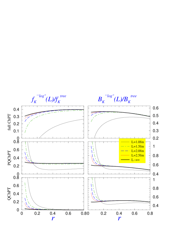
Figure 1: From top to bottom, we plot the chiral logarithmic corrections as predicted in full, partially quenched ($r_{\rm sea}=m_{\rm sea}/m_{s}^{\rm phys}=0.5$) and quenched ChPT, respectively, as functions of the light valence quark mass $r=m_{q}/m_{s}$, where the strange quark mass is fixed to its physical value. In each plot the thick line corresponds to the physical (infinite volume) chiral logarithm, whereas the other four curves correspond to the logarthmic contributions computed in the finite volume $V=L^{3}$, where for $L$ we choose the values shown in the legend. The renormalisation scale is chosen to be $\mu=1$ GeV.

However, by decreasing the quark mass, the sensitivity to the finiteness of the lattice box of side $L$ becomes more pronounced. Moreover, the finite volume effects modify the nonlinear light quark dependence in the same way, i.e., they enhance the chiral logs. The problem is that the nonlinearity induced by the finite volume is larger than that due to the presence of physical chiral logarithms. To illustrate that statement, in fig. 1 we plot the chiral log contributions in the finite and infinite volumes, by using the expressions presented in the previous section for both $f_{K}$ and $B_{K}$ in all three versions of ChPT. From that plot we see that it is very difficult to distinguish between physical chiral logarithms (thick curves) and the finite volume effect, even if one manages to work with very light quarks on the currently used lattice volumes. For smaller masses, at which the chiral logarithms are expected to set in, the finite volume effects completely overwhelm the physical non-linearity.

A possible way out would be to fit the lattice data to the finite volume forms (see Sec. 3) and not to those of the infinite volume, given in Sec. 2. That, of course, is legitimate if one assumes the validity of the NLO ChPT formulae. Finally, the curves corresponding to $L=1$ fm should be taken cautiously because this volume may be too small for ChPT to set in, as recently discussed in ref. [16].

5 Finite volume corrections

In this section we combine the formulae derived in Secs. 2 and 3 to discuss the shift of $f_{K}$ and $B_{K}$ induced by the finite volume effects. Before embarking on this issue, we first briefly remind the reader about the similar shift in the case of the pion mass where, for large $L$, the one-loop ChPT expression indeed agrees with the general formula derived by Lüscher in ref. [17]. Since the analogous general formulae for $f_{K}$ and $B_{K}$ do not exist, we will derive them by taking the large $L$ limit of our one-loop ChPT formulae.

5.1 Contact with Lüscher’s formula

To make contact with Lüscher’s formula, we subtract the one-loop chiral correction to the pion mass (squared) as obtained in the full (unquenched) ChPT in infinite volume from the one obtained in a finite volume. By evaluating the sums, as described in the previous section, we have

$$m_{\pi}^{2}(\infty)=2B_{0}m_{q}\left\{1+{1\over(4\pi f)^{2}}\left[m_{\pi}^{2}\log\left({m_{\pi}^{2}\over\mu^{2}}\right)-{1\over 3}m_{\eta}^{2}\log\left({m_{\eta}^{2}\over\mu^{2}}\right)\right]\right\}\,,$$

$$m_{\pi}^{2}(L)=2B_{0}m_{q}\left[1+{1\over 2f^{2}L^{3}}\sum_{\vec{q}}\left({1\over\omega_{\pi}}\ -\ {1\over 3\ \omega_{\eta}}\right)\right]\,,$$

$$\Longrightarrow {\Delta m_{\pi}^{2}\over m_{\pi}^{2}}\equiv{m_{\pi}^{2}(L)-m_{\pi}^{2}(\infty)\over m_{\pi}^{2}(\infty)}={1\over 2f^{2}}\left[\xi_{1/2}(L,m_{\pi})-{1\over 3}\xi_{1/2}(L,m_{\eta})\right]\,,$$ (35)

which coincides with the result of ref. [18].  Analytic terms in $m_{\pi}^{2}(\infty)$ and $m_{\pi}^{2}(L)$ were omitted since they cancel in $(\Delta m_{\pi}^{2})/m_{\pi}^{2}$.

To recover Lüscher’s formula, one takes the limit $L\to\infty$, which amounts to using the asymptotic form (34) in eq. (5.1),

$${\Delta m_{\pi}\over m_{\pi}}\simeq{3\over 2}\left({m_{\pi}\over f}\right)^{2}{e^{-m_{\pi}L}\over(2\pi m_{\pi}L)^{3/2}}\,,$$ (36)

where only the leading exponential has been kept. The benefit of eq. (5.1) is that it offers insight into the subleading terms, suppressed by higher powers in $e^{-m_{\pi}L}$ in Lüscher’s formula. In the range of volumes in which the right-hand side of eq. (36) becomes sizable, the subleading exponential terms cannot be neglected and the formula (5.1) has to be used. For the volumes currently used in lattice simulations, these corrections are important if one is to work with very light pions.

Before closing this subsection, two important comments are in order, though. First, Lüscher’s formula relates the finite volume shift of the pion mass to the $\pi\!-\!\pi$ scattering amplitude. Equation 36 refers to the tree level $\pi\!-\!\pi$ scattering amplitude. A recent study in ref. [16] shows that the inclusion of the NLO chiral corrections to the $\pi\!-\!\pi$ scattering amplitude produces a sizable correction to eq. (36). It is, however, not clear whether or not such a conclusion persists in the full (nonasymptotic) case, i.e., eq. (5.1). It is even less clear if such a conclusion carries over to other quantities. To resolve that issue, one should compute the finite volume two-loop chiral correction to the pion mass (and to other quantities), which is beyond the scope of the present work. It is clear, however, that before this point is clarified, one cannot safely use the one-loop calculation to correct for the finite volume effects. At present the one-loop ChPT finite volume expressions are useful for making a rough estimate of the finite volume corrections. The second comment is that the derivation of Lüscher’s formula relies crucially on unitarity. Since the unitarity in the partially quenched and quenched theories is lost, Lüscher’s formula is not valid in these theories.

5.2 Finite volume corrections to $f_{K}$

We now use the expressions for the decay constant $f_{K}$, derived in the infinite [eqs. (11)-(13)] and finite [eqs. (19)-(21)] volume cases, to estimate the shift in $f_{K}$ due to the finiteness of the volume. For that purpose we define

$${\Delta f_{K}\over f_{K}}\equiv{f_{K}(L)-f_{K}(\infty)\over f_{K}(\infty)}\,.$$ (37)

It should be clear that the analytic terms multiplied by the low energy constants (omitted in Secs. 2 and 3) cancel in the ratio (37).  Finally, we have

$$\left({\Delta f_{K}\over f_{K}}\right)^{\rm ChPT}=-\frac{3}{8\,f^{2}}\,\left[{{\xi}_{\frac{1}{2}}}(L,{m_{\pi}})\ +\ {2}\ {{\xi}_{\frac{1}{2}}}(L,{m_{K}})\ +\ {{\xi}_{\frac{1}{2}}}(L,{m_{\eta}})\right]\,,$$ (38)

$$\left({\Delta f_{K}\over f_{K}}\right)^{\rm PQChPT} = \frac{1}{8\,f^{2}}\,\left\{\frac{m_{SS}^{2}-m_{\pi}^{2}}{2}{{\xi}_{\frac{3}{2}}}(L,{m_{\pi}})+\frac{m_{SS}^{2}-m_{22}^{2}}{2}{{\xi}_{\frac{3}{2}}}(L,{m_{22}})-4\ \left[{{\xi}_{\frac{1}{2}}}(L,{m_{13}})\right.\right.$$ (39)

$$\qquad\quad\left.\left.+{{\xi}_{\frac{1}{2}}}(L,{m_{23}})\right]+\frac{m_{SS}^{2}-m_{K}^{2}}{m_{K}^{2}-m_{\pi}^{2}}\left[{{\xi}_{\frac{1}{2}}}(L,{m_{22}})-{{\xi}_{\frac{1}{2}}}(L,{m_{\pi}})\right]\right\}\,,$$

$$\left({\Delta f_{K}\over f_{K}}\right)^{\rm QChPT} = -\frac{1}{12\,f^{2}}\left\{\frac{\alpha_{0}\,m_{K}^{2}-m_{0}^{2}}{m_{K}^{2}-m_{\pi}^{2}}\,\left[{{\xi}_{\frac{1}{2}}}(L,{m_{22}})-{{\xi}_{\frac{1}{2}}}(L,{m_{\pi}})\right]\right.$$ (40)

$$\left.-\frac{m_{0}^{2}-\alpha_{0}\,m_{22}^{2}}{2}\,{{\xi}_{\frac{3}{2}}}(L,{m_{22}})-\frac{m_{0}^{2}-\alpha_{0}\,m_{\pi}^{2}}{2}\,{{\xi}_{\frac{3}{2}}}(L,{m_{\pi}})\right\}\,.$$

Similar expressions in full and quenched ChPT, but for the case in which the kaon consists of two quarks degenerate in mass, were obtained in ref. [6]. For the general nondegenerate case and for PQChPT, the above formulae are new. In ref. [19], the finite volume terms are taken into account while computing the full ChPT corrections to $f_{K}$ relevant to the lattice computation of this quantity with staggered quarks.

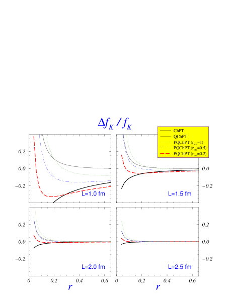
Figure 2: The finite volume corrections to $f_{K}$ in full, partially quenched and quenched theory, eqs. (38),(39),(40), respectively. The partially quenched case that we consider is the one with $N_{\rm f}=2$ dynamical quarks degenerate in mass for which we take $r_{\rm sea}=m_{\rm sea}/m_{s}^{\rm phys}=1,0.5,0.2$. Each plot corresponds to a different value of the size of the side of the box $L$, indicated in the plots. We keep the same scale, to better appreciate the reduction of the finite volume effects as $L$ is increased.

In fig. 2, we illustrate the finite volume effects as predicted by the above formulae. Since the mass of the strange quark is directly simulated on the lattice, we keep it fixed. As for the light quark we define, $r=m_{q}/m_{s}^{\rm phys}$, which we then vary as $r\in[r_{u/d},1]$, where $r_{u/d}=(m_{u}+m_{d})/2m_{s}=0.04$ [20]. We also use the Gell-Mann–Oakes–Renner (GMOR) and Gell-Mann–Okubo formulae, namely,

$$m_{\pi}^{2}=2B_{0}m_{s}r\ ,\quad m_{K}^{2}=2B_{0}m_{s}{r+1\over 2}\ ,\quad m_{\eta}^{2}=2B_{0}m_{s}{r+2\over 3}\ .$$ (41)

The illustration in fig. 2 is made for realistic volumes currently used in lattice simulations: $L\in[1\ {\rm fm},\ 2.5\ {\rm fm}]$. In obtaining the quenched curves, we assume $m_{0}=0.6$ GeV and $\alpha_{0}=0.05$. The curves are insensitive to the value of $\alpha_{0}$. On the other hand, the effect shown in fig. 2 becomes pronounced if $m_{0}$ is increased to $m_{0}=0.65$ GeV or $m_{0}=0.7$ GeV, values sometimes also quoted in the literature.

From fig. 2 we see that the finite volume effects become more pronounced as the light quark gets closer to the physical $u/d$ quark mass. In particular, they result in shifting the quenched $f_{K}$ toward a larger value, wheras the shift of $f_{K}$ in full (unquenched) QCD is opposite, i.e., the finite volume effects lower the value of $f_{K}$. The partially unquenched cases lie between the two. We see that the quenched chiral logs become dominant as soon as the mass of the valence quark becomes lighter than the sea-quark mass. We did not plot the case when the valence and sea quarks are degenerate since such a curve is very close to the full ChPT case. It is worth noticing that in the region of $r\lesssim 0.2$ the finite volume effects for the partially quenched $f_{K}$, with $r_{\rm sea}=1$, are larger than for the quenched case.

5.3 Finite volume corrections to $B_{K}$

We proceed in a completely analogous way as in the last subsection and define

$${\Delta B_{K}\over B_{K}}\equiv{B_{K}(L)-B_{K}(\infty)\over B_{K}(\infty)}\,.$$ (42)

The corresponding ChPT expressions read

$$\left({\Delta B_{K}\over B_{K}}\right)^{\rm ChPT} = \frac{1}{4f^{2}}\left[-\frac{m_{K}^{2}+m_{\pi}^{2}}{m_{K}^{2}}\ {{\xi}_{1/2}}(L,{m_{\pi}})+2m_{K}^{2}\ {{\xi}_{3/2}}(L,{m_{K}})\right.$$ (43)

$$\qquad\,\left.-\left(7-\frac{m_{\pi}^{2}}{m_{K}^{2}}\right)\ {{\xi}_{1/2}}(L,{m_{\eta}})\right]\,,$$

$$\left({\Delta B_{K}\over B_{K}}\right)^{\rm PQChPT}\!\!\!\! = -\frac{1}{2f^{2}}\left[\left({5m_{K}^{2}-m_{\pi}^{2}\over 2m_{K}^{2}}\ -\ {m_{SS}^{2}-m_{K}^{2}\over m_{K}^{2}-m_{\pi}^{2}}\right)\ {{\xi}_{1/2}}(L,{m_{22}})\right.$$ (44)

$$\quad+\left({m_{K}^{2}+m_{\pi}^{2}\over 2m_{K}^{2}}\ +\ {m_{SS}^{2}-m_{\pi}^{2}\over m_{K}^{2}-m_{\pi}^{2}}\right)\ {{\xi}_{1/2}}(L,{m_{\pi}})$$

$$\quad+\,\frac{\left(m_{K}^{2}+m_{22}^{2}\right)\,\left(m_{22}^{2}-m_{SS}^{2}\right)}{4m_{K}^{2}}\,{{\xi}_{3/2}}(L,{m_{22}})$$

$$\quad\left.-m_{K}^{2}\ {{\xi}_{3/2}}(L,{m_{K}})-\,\frac{\left(m_{K}^{2}+m_{\pi}^{2}\right)\,\left(m_{SS}^{2}-m_{\pi}^{2}\right)}{4m_{K}^{2}}\,{{\xi}_{3/2}}(L,{m_{\pi}})\right]\,,$$

$$\left({\Delta B_{K}\over B_{K}}\right)^{\rm QChPT}\!\!\!\!\!\! = \frac{1}{2f^{2}}\left\{\left[{2m_{0}^{2}\over 3(m_{K}^{2}-m_{\pi}^{2})}-{3m_{K}^{2}-m_{\pi}^{2}\over m_{K}^{2}}-{\alpha_{0}\over 3}\left({m_{K}^{2}+m_{\pi}^{2}\over m_{K}^{2}-m_{\pi}^{2}}+{m_{\pi}^{2}\over m_{K}^{2}}\right)\right]\ {{\xi}_{1/2}}(L,{m_{22}})\right.$$ (45)

$$\quad-\left[{2m_{0}^{2}\over 3(m_{K}^{2}-m_{\pi}^{2})}+{m_{K}^{2}+m_{\pi}^{2}\over m_{K}^{2}}-{\alpha_{0}\over 3}\left({m_{K}^{2}+m_{\pi}^{2}\over m_{K}^{2}-m_{\pi}^{2}}+{m_{\pi}^{2}\over m_{K}^{2}}\right)\right]\ {{\xi}_{1/2}}(L,{m_{\pi}})$$

$$\quad+\frac{\left(m_{K}^{2}+m_{22}^{2}\right)\,\left(m_{0}^{2}-\alpha_{0}\ m_{22}^{2}\right)}{6\ m_{K}^{2}}\,{{\xi}_{3/2}}(L,{m_{22}})+{m_{K}^{2}}\ {{\xi}_{3/2}}(L,{m_{K}})$$

$$\quad\left.+\frac{\left(m_{K}^{2}+m_{\pi}^{2}\right)\,\left(m_{0}^{2}-\alpha_{0}\ m_{\pi}^{2}\right)}{6\ m_{K}^{2}}\ {{\xi}_{3/2}}(L,{m_{\pi}})\right\}\,.$$

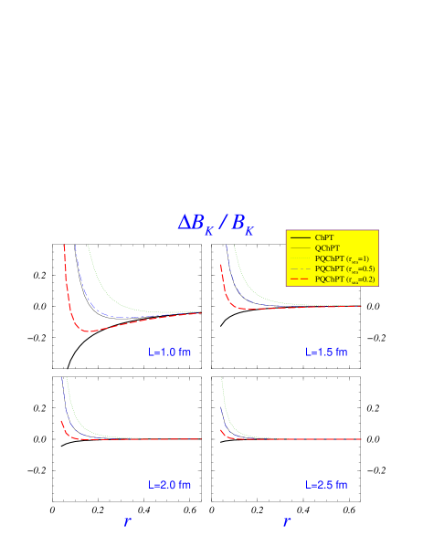
Figure 3: The finite volume corrections to $B_{K}$ in full, partially quenched and quenched theory, eqs. (43),(44),(45), respectively.

The illustration, similar to the one discussed in the previous subsection, is provided in fig. 3. We observe that, as in the case of $f_{K}$, the finite volume effects become pronounced as the light valence quark is lowered toward the physical $u/d$ quark mass. Moreover, they have a tendency to enhance the nonlinearities which would otherwise be attributed to the physical chiral logarithms. 

5.4 Asymptotic $L\to\infty$ formulae for $f_{K}$ and $B_{K}$

As discussed at the beginning of this section, the difference of the one-loop ChPT formulae for the pion mass in the finite and infinite volume (i) reproduces Lüscher’s general formula at LO, and (ii) allows one to estimate the size of the corrections suppressed in Lüscher’s formula. Similar asymptotic formulae for $f_{K}$ and $B_{K}$ can be obtained from our full ChPT expressions for $\Delta f_{K}/f_{K}$ and $\Delta B_{K}/B_{K}$, i.e., eqs. (38) and (43), respectively. By using the asymptotic form (34), we get

$${\Delta f_{K}\over f_{K}}\simeq-{9\over 4}\left({m_{\pi}\over f}\right)^{2}{e^{-m_{\pi}L}\over(2\pi m_{\pi}L)^{3/2}}\,,\quad{\Delta B_{K}\over B_{K}}\simeq-{3\over 2}\frac{m_{K}^{2}+m_{\pi}^{2}}{m_{K}^{2}}\left({m_{\pi}\over f}\right)^{2}{e^{-m_{\pi}L}\over(2\pi m_{\pi}L)^{3/2}}\,.$$ (46)

To check how good an approximation these formulae are to the complete ones, given in eqs. (38) and (43), we made a numerical comparison of the two, and conclude that for volumes larger than $(2\ {\rm fm})^{3}$ and masses $r\gtrsim 1/4$, eq. (46) is an excellent approximation. Otherwise, i.e., in the region in which the finite volume effects become important, the asymptotic forms (46) become inadequate and eqs. (38) and (43) should be used. We note, in passing, that formulae similar to those in eq. (46), but in the quenched case, were reported in refs. [5, 6].

6 Summary

In this work we computed the one-loop chiral corrections to the decay constant $f_{K}$ and to the bag parameter $B_{K}$ in all three versions of ChPT, i.e., full, quenched, and partially quenched. After working out the formulae in both infinite and finite volumes, we were able to discuss the impact of the finite volume effects on the chiral behavior of $f_{K}$ and $B_{K}$. We show that in most situations the physical chiral logarithms are completely drowned in the finite volume artefacts. In other words, unambiguously disentangling the physical chiral logarithms from the finite volume lattice artefacts does not appear to be feasible unless very large volumes are used.

We also discussed the shift of $f_{K}$ and $B_{K}$ induced by the finiteness of the volume. In our discussion we fix the strange quark in the kaon to its physical mass $m_{s}$, whereas the mass of the light quark is varied between $m_{s}/25$ and $m_{s}$. This mimics the current lattice QCD studies in which the strange quark is directly accessed on the lattice while the accessible light quarks have $r=m_{q}/m_{s}\in(0.5,1)$, so that an extrapolation to the physical $r_{u/d}=0.04$ is necessary.

The results of our calculation indicate that for $r\gtrsim 0.25$ the finite volume effects are very small as long as $L\gtrsim 2$ fm. In that region we provide a simple asymptotic formula which is an accurate approximation of the full ChPT expressions.

From our formula it is also obvious that the finite volume corrections to $f_{K}$ and $B_{K}$ are different in quenched and partially quenched QCD from those obtained in full QCD. Therefore, if in practical numerical simulations one wants to see only the effects of (un)quenching, the finite volume effects must be kept under control.

References

• [1] C. Aubin et al. [MILC Collaboration], hep-lat/0309088.
• [2] M. Battaglia et al., hep-ph/0304132.
• [3] J. Gasser and H. Leutwyler, Nucl. Phys. B 250 (1985) 465.
• [4] J. F. Donoghue, E. Golowich and B. R. Holstein, “Dynamics Of The Standard Model”, Cambridge Monogr. Part. Phys. Nucl. Phys. Cosmol.  2 (1992) 1. H. Leutwyler, “Chiral dynamics”, hep-ph/0008124; A. Pich, Rep. Prog. Phys.  58 (1995) 563 [hep-ph/9502366]; G. Ecker, “Strong interactions of light flavours”, hep-ph/0011026; U. G. Meissner, Rep. Prog. Phys.  56 (1993) 903 [hep-ph/9302247]; G. Colangelo, G. Isidori, “An introduction to ChPT”, hep-ph/0101264.
• [5] C. W. Bernard and M. F. Golterman, Phys. Rev. D 46 (1992) 853 [hep-lat/9204007].
• [6] S. R. Sharpe, Phys. Rev. D 46 (1992) 3146 [hep-lat/9205020].
• [7] C. W. Bernard and M. F. Golterman, Phys. Rev. D 49 (1994) 486 [hep-lat/9306005].
• [8] S. R. Sharpe and N. Shoresh, Phys. Rev. D 64 (2001) 114510 [hep-lat/0108003].
• [9] S. R. Sharpe, Phys. Rev. D 56 (1997) 7052 [Erratum-ibid. D 62 (2000) 099901] [hep-lat/9707018].
• [10] M. F. Golterman and K. C. Leung, Phys. Rev. D 57 (1998) 5703 [hep-lat/9711033].
• [11] J. F. Donoghue, E. Golowich and B. R. Holstein, Phys. Lett. B 119 (1982) 412.
• [12] J. Bijnens and J. Prades, JHEP 0001 (2000) 002 [hep-ph/9911392]; S. Peris and E. de Rafael, Phys. Lett. B 490 (2000) 213 [hep-ph/0006146].
• [13] M. F. Golterman and K. C. Leung, Phys. Rev. D 56 (1997) 2950 [hep-lat/9702015].
• [14] I.S. Gradshteyn, I.M. Ryzhik, Table of Integrals, Series, and Products, 5th ed. San Diego, CA: Academic, 1994 (see page 921).
• [15] M.J. Lighthill, Introduction to Fourier analysis and generalised functions, Cambridge Univ.Press, 1958 (see page 69).
• [16] G. Colangelo and S. Durr, hep-lat/0311023.
• [17] M. Luscher, Commun. Math. Phys.  104 (1986) 177.
• [18] J. Gasser and H. Leutwyler, Phys. Lett. B 184 (1987) 83.
• [19] C. Aubin and C. Bernard, Phys. Rev. D 68 (2003) 074011 [hep-lat/0306026].
• [20] H. Leutwyler, Phys. Lett. B 378 (1996) 313 [hep-ph/9602366].