IFUP-TH 2003/29, UPRF-2003-20
The two-dimensional Wess-Zumino model in the Hamiltonian lattice formulation

Abstract

We investigate a Hamiltonian lattice version of the two-dimensional Wess-Zumino model, with special emphasis to the pattern of supersymmetry breaking. Results are obtained by Quantum Monte Carlo simulations and Density Matrix Renormalization Group techniques.

1 INTRODUCTION AND PRESENTATION OF THE MODEL

Most studies of lattice field theory are performed in the well-known Lagrangian formalism, discretizing both space and time. We feel that it is important not to neglect the Hamiltonian formalism [1], which affords, e.g., a more immediate approach to the mass spectrum and to the implementation of fermions; numerical methods are quite different in the Lagrangian and in Hamiltonian formalism, and comparison between the two can provide important test of the methods as well as of universality.

We chose to study an Hamiltonian lattice version of the two-dimensional Wess-Zumino model, described in Ref. [2]; the model enjoys an exact 1-dimensional supersymmetry algebra $H=Q^{2}$, which suffices to preserve a few key properties of the continuum model (which has a full 2-dimensional supersymmetry): the energy spectrum is non-negative; states of nonzero energy appear in boson-fermion doublets; spontaneous supersymmetry breaking is equivalent to a strictly positive ground-state energy $E_{0}$.

The model is parametrized by the prepotential, an arbitrary polynomial in the bosonic field $V(\phi)$; the model is superrenormalizable, and the only renormalization needed is the normal ordering of $V(\phi)$.

It is interesting to notice that the strong-coupling expansion predicts supersymmetry breaking if and only if the degree of the prepotential $V$ is even, while perturbation theory predicts supersymmetry breaking if and only if $V$ has no zeroes; the two contitions are quite different in the case, e.g., of quadratic $V$, and it is interesting to study the crossover from strong to weak coupling.

2 NUMERICAL METHODS

A standard numerical simulation technique that can be applied to the model we are interested in is the Green Function Monte Carlo (GFMC) algorithm [3]. The interested reader may find a description of GFMC applied to the present problem in Ref. [2]; we only remark here that the GFMC algorithm generates a stochastic representation of the ground-state wavefunction, from which expectation values of observables can be computed; the variance of observables can be kept under control by the introduction of a population of $K$ walkers (field configurations), and an extrapolation to $K\to\infty$ of the result is required.

Another numerical approach which has been applied with success to 1-dimensional Hamiltonian models is the Density-Matrix Renormalization Group (DMRG) [4, 5]; the parameters of the algorithm are the dimension $S$ to which the local (1-site) Hilbert space is truncated, and the number $M$ of eigenstates of the density matrix of the full system that are retained; extrapolation to $M\to\infty$ and $S\to\infty$ is needed. DMRG is a deterministic algorithm and does not suffer from the sign problem; it is possible to obtain directly infinite-volume results.

3 NUMERICAL RESULTS

The most interesting property of the model is the pattern of supersymmetry breaking, especially in the case of quadratic prepotential; we study the case of even prepotential $V(\phi)=\lambda_{2}\phi^{2}+\lambda_{0}$, for which the strong-coupling expansion predicts supersymmetry breaking for all values of $\lambda_{0}$, while perturbation theory predicts unbroken supersymmetry for $\lambda_{0}<0$.

The model enjoys an approximate $\phi_{m}\to-\phi_{m}$, $n_{m}\to 1-n_{m}$ symmetry (“parity”); supersymmetry breaking is incompatible with parity breaking [6], and it is reasonable to expect only two phases: unbroken supersymmetry and broken parity for $\lambda_{0}<\lambda_{c}$, broken supersymmetry and unbroken parity for $\lambda_{0}>\lambda_{c}$.

An analysis of the approach to the continuum limit, along a trajectory of “constant physics” in the phase of broken supersymmetry was presented in Ref. [7]. In the present paper, we study the model varying $\lambda_{0}$ at fixed $\lambda_{2}=0.5$.

We monitor supersymmetry breaking by looking at the ground-state energy density $E_{0}/L$. Infinite-volume DMRG results are shown in Fig. 1; we remind that they must be extrapolated to $S\to\infty$ and $M\to\infty$.

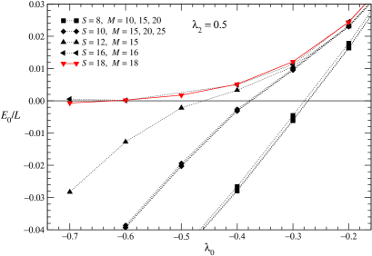
Figure 1: Ground-state energy density vs. $\lambda_{0}$ obtained by DMRG with different values of $S$ and $M$.

GFMC results are extrapolated to $L\to\infty$ and $K\to\infty$ by a best fit to the form

$${E_{0}\over L}={\cal E}+{a\over L}+{b\over L^{2}}+{c\over K^{\nu}}+{d\over LK^{\nu}},$$

which gives a good $\chi^{2}$ (at least for $\lambda_{0}>-0.46$); the fit gives $\nu\simeq 0.5$, signaling a slow convergence to $K\to\infty$ (to stabilize the fit, we ran with $K$ up to 5000 for our smallest lattice $L=22$). ${\cal E}$ is plotted in Fig. 2, together with DMRG results for the highest values of $S$ and $M$; the agreement is remarkable.

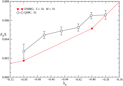
Figure 2: Ground-state energy density vs. $\lambda_{0}$ obtained by DMRG with different values of $S$ and $M$.

We study parity symmetry breaking looking at the Binder cumulant

$$B={\langle M^{4}\rangle\over\langle M^{2}\rangle^{2}},\qquad M=\sum_{n}\phi_{n},$$

where the sum excludes sites closer to the border than (typically) 6; a good estimate of the transition point is the intersection of the curves $B$ vs. $\lambda_{0}$ obtained at different values of $L$. GFMC results are shown in Figs. 3 and 4; they are quite sensitive to $K$ and not very precise.

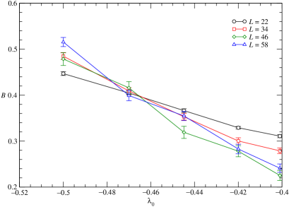
Figure 3: The Binder cumulant $B$ for $K=200$.

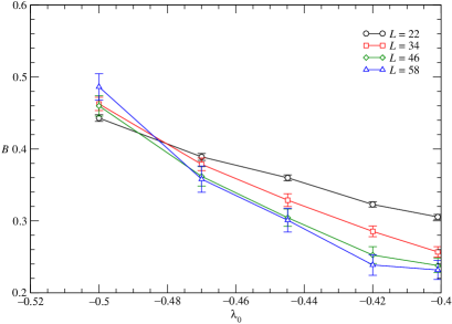
Figure 4: The Binder cumulant $B$ for $K=500$.

Therefore, we follow a different strategy and consider the connected correlation function $G_{d}=\langle\phi_{n}\phi_{m}\rangle_{c}$ averaged over all $n,m$ pairs with $|m-n|=d$, excluding pairs for which $m$ or $n$ is closer to the border than (typically) 6; since we are using staggered fermions, even and odd $d$ may correspond to different physical channels. The correlation function is quite different in the two phases: for $\lambda_{0}\gg\lambda_{c}$, there is a marked difference between even and odd distances, and $G_{d}$ is short-ranged; for $\lambda_{0}\ll\lambda_{c}$, even and odd distances are equivalent, and $G_{d}$ appears to be long-ranged. We fit $G_{d}$ to the form $\exp(a+bd)+c$, separately for even and odd $d$; the best fits give a good $\chi^{2}$ if we remove the smallest distances, typically $d\leq 3$ for the odd channel and $d\leq 6$ for the even channel. The difference between the two phases is apparent, e.g., in the plot of $c$ vs. $\lambda_{0}$, presented in Fig. 5.

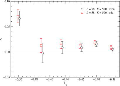
Figure 5: The long-distance correlation of $\phi$ vs. $\lambda_{0}$ for $L=58$ and $K=500$.

References

- [1] J. Kogut, L. I. Susskind, Phys. Rev. D11 (1975) 395; J. Kogut, Rev. Mod. Phys. 51 (1979) 659.
- [2] M. Beccaria, M. Campostrini, A. Feo, e-print hep-lat/0109005, in Quantum Monte Carlo, M. Campostrini, M. P. Lombardo, and F. Pederiva eds., ETS, Pisa, 2001.
- [3] W. von der Linden, Phys. Rept. 220 (1992) 53.
- [4] C. Zhang, E. Jeckelmann, S. R. White, Phys. Rev. Lett. 80 (1998) 2661;
- [5] K. Hallberg, e-print cond-mat/0303557, to appear in Theoretical Methods for Strongly Correlated Electrons, D. Senechal, A.-M. Tremblay and C. Bourbonnais eds., CRM Series in Mathematical Physics, Springer, New York, 2003.
- [6] E. Witten, Nucl. Phys. B202 (1982) 253.
- [7] M. Beccaria, M. Campostrini, A. Feo, Nucl. Phys. B (Proc. Suppl.) 119 (2002) 891.