An analysis of the vector meson spectrum from lattice QCD

Abstract

We re-analyse meson sector data from the CP–PACS collaboration’s dynamical simulations [1]. Our analysis uses several different approaches, and compares the standard näive linear fit with the Adelaide Anzatz. We find that setting the scale using the J parameter gives remarkable agreement among data sets. Our predictions for the $\rho$ and $\phi$ masses have very small statistical errors, $\sim 3$ MeV, but the discrepancy between the different fitting approaches is $\sim 40$ MeV.

1 Introduction

We study the chiral extrapolation of the vector meson data from CP–PACS [1]. We do not have access to CP-PACS original data, so we produced Gaussian distributions with central values and FWHM’s equal to the quoted central values and errors respectively. Our data is uncorrelated throughout and we only fit to degenerate data, i.e. $\kappa_{\rm val}^{1}=\kappa_{\rm val}^{2}$. The CP–PACS data used is from mean–field improved Wilson fermions with improved glue at four different $\beta$ values. For each $\beta$ value there are four different $\kappa_{\rm sea}$ values, giving sixteen independent ensembles.The physical volume was held fixed at $La\approx 2.5$ fm for the $\beta=1.80,1.95$ and $2.10$, but the $\beta=2.20$ ensemble had a slightly smaller physical volume. A graphical overview of the CP–PACS data is given in Figure 1. We also fit to CP–PACS quenched data for comparison.

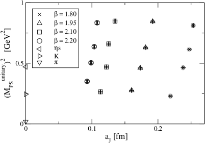
Figure 1: A Graphical overview of the CP–PACS data. Note that here the scale is set using the inverse lattice spacing determined from the J parameter [2].

2 Fitting analysis

2.1 Summary of analysis techniques

Our chiral extrapolation approach is based upon converting all masses into physical units prior to any extrapolation being performed. An alternative approach would be to extrapolate dimensionless masses (in lattice units) [1]. Our method has the following two advantages:

• Different ensemble’s data can be combined together in a global fit.

• Dimensionful mass predictions from lattice simulations are effectively mass ratios, and hence one would expect some of the systematic and statistical errors to cancel.

2.2 Fitting functions

In our chiral extrapolations we use the näive linear fit, Eq.(2.2), as well as the Adelaide Anzatz, [3] Eq.(2.2).

$$M_{V}(\beta,\kappa_{\rm sea};\kappa_{\rm val},\kappa_{\rm val})=$$

$$C_{0}+C_{2}M^{2}_{PS}(\beta,\kappa_{\rm sea};\kappa_{\rm val},\kappa_{\rm val}).$$ (1)

$$M_{V}(\beta,\kappa_{\rm sea};\kappa_{\rm val},\kappa_{\rm val})=$$

$$C_{0}+C_{2}M^{2}_{PS}(\beta,\kappa_{\rm sea};\kappa_{\rm val},\kappa_{\rm val})~{}+$$

$$\frac{1}{2}\frac{\left[\Sigma^{\rho}_{\pi\pi}+\Sigma^{\rho}_{\pi\omega}\right]}{(C_{0}+C_{2}M^{2}_{PS}(\beta,\kappa_{\rm sea};\kappa_{\rm val},\kappa_{\rm val})}$$ (2)

where the Self Energies are defined as $\Sigma^{\rho}_{\pi\pi}=\Sigma^{\rho}_{\pi\pi}(M^{2}_{PS}(\beta,\kappa_{\rm sea};\kappa_{\rm sea},\kappa_{\rm val}))$ and $\Sigma^{\rho}_{\pi\omega}=\Sigma^{\rho}_{\pi\omega}(M^{2}_{PS}(\beta,\kappa_{\rm sea};\kappa_{\rm sea},\kappa_{\rm val}))$. $M_{V(PS)}$ is the vector(pseudo-scalar) meson mass. $\beta$ and $\kappa_{\rm sea}$ refer to the sea structure (i.e. the gauge coupling and sea quark hopping parameter) and $\kappa_{\rm val}$ refers to the valence quark hopping parameters.

The Adelaide method relies on a parameter $\Lambda_{\pi\omega}$ [3]. We use the value of $\Lambda_{\pi\omega}=630$ MeV taken from [3]. The value of $\Lambda_{\pi\omega}$ is highly constrained by the lightest data point in the $M_{V}$ versus $M_{PS}^{2}$ plot, and since the data used in [3] includes a much lighter point than in this study, we use its value of $\Lambda_{\pi\omega}$.

2.3 Individual ensemble fits

Our first method for obtaining physical masses involves determining fitting parameters, $C_{0}$ and $C_{2}$, for each of the 16 data sets and then performing a continuum extrapolation to those. Figure 2 displays the $C_{0}$ values and motivates a continuum extrapolation of the form in Eq.(3).

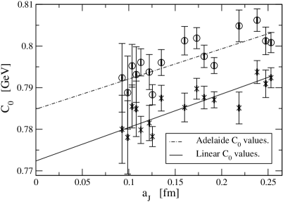
Figure 2: An example of a continuum extrapolation performed to fitting parameters obtained from the sixteen different data sets.

$$C_{0,2}(a)=C_{0,2}^{cont}+X_{0,2}\;a_{J}.$$ (3)

Table 1 lists the results for these fits.

	$C_{0}^{cont.}$	$X_{0}$	$\chi^{2}_{0}/d.o.f.$	$C_{2}^{cont.}$	$X_{2}$	$\chi^{2}_{2}/d.o.f.$
	[GeV]	[GeV/fm]		[GeV-1]	[GeV-1/fm]
Linear-fit	$0.772\pm{3}$	$8\pm{2}\times 10^{-2}$	$1.10/14$	$0.473\pm{6}$	$-0.27\pm{3}$	$1.86/14$
Adelaide-fit	$0.785\pm{3}$	$7\pm{2}\times 10^{-2}$	$2.01/14$	$0.462\pm{6}$	$-0.26\pm{3}$	$1.39/14$

Table 1: The coefficients obtained from the continuum extrapolation of the parameters obtained from the 16 individual fits using Eq.(3).

2.4 Global fits

Figure 3 plots the vector meson mass against the pseudo–scalar mass squared (in physical units) for all of the data from all of the ensembles. As can be seen the data lies on a near universal line. This motivates an analysis which combines all of the degenerate data into one global fit.

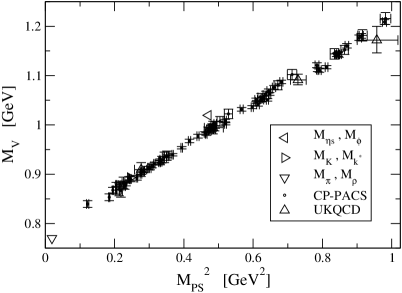
Figure 3: A plot of $M_{V}$ versus $M_{PS}^{2}$ for the degenerate CP-PACS dataset showing that the data lies on a near universal line. Also plotted are the three experimental data points, and the unitary data from UKQCD [4]. Note that the scale for the lattice data was set using the method of [2].

To underline the near universal nature of the data we plot the relative spread of the data using Eq.4.

$$\mbox{spread}=\frac{M_{V}^{data}}{C_{0}+C_{2}M_{PS}^{2}}$$ (4)

Where $C_{0}+C_{2}M_{PS}^{2}$ is a simple fit through the data in Figure 3. In Figure 4 we see that the spread is at the 1% level or less. Note that this simple linear fit is not used in any further analysis. Also note that the scale is set from J [2] and hence the data must pass through the (M${}_{K}*$ , M_K) point.

Figure 4: A plot showing the relative spread in $M_{V}$ versus $M^{2}_{PS}$ for the degenerate CP–PACS data set.

When grouping the different ensembles together we must allow for some (small) variation with the lattice spacing. We do this by modifying the linear and Adelaide fitting functions. By substituting Eq.(5) into Eqs.(2.2 & 2.2) respectively. Table 2 lists the results of these fits.

$$C_{0,2}\rightarrow C^{\prime}_{0,2}+X^{\prime}_{0,2}a.$$ (5)

	$C^{\prime}_{0}$	$X^{\prime}_{0}$	$C^{\prime}_{2}$	$X^{\prime}_{2}$	$\chi^{2}/d.o.f.$
	[GeV]	[GeV/fm]	[GeV-1]	[GeV-1/fm]
Linear–fit	$0.772\pm{3}$	$8\pm{2}\times 10^{-2}$	$0.474\pm{6}$	$-0.28\pm{3}$	$43/76$
Adelaide–fit	$0.784\pm{3}$	$7.8\pm{16}\times 10^{-2}$	$0.466\pm{6}$	$-0.28\pm{3}$	$58/76$

Table 2: The coefficients obtained from a global fit of all the $M_{V}$ data against $M^{2}_{PS}$ using the linear-O(a), Eq.(1), and Adelaide-O(a), Eq.(2), fits, both incorporating Eq.(5).

3 Conclusions

To conclude, Table 3 lists our mass estimates for the $\rho$ and $\phi$ mesons. We see that our interpretation of the Adelaide Anzatz underestimates M_ρ presumably due to a poorly tuned $\Lambda_{\pi\omega}$ value. We also note the following:

• Setting the scale using J gives remarkable agreement among data sets.

• The (statistical) errors in the mass estimates are tiny.

• The discrepancies between the various fitting procedures is much larger than the statistical errors listed.

• Note that for the global linear fit that incorporates the $Xa$ correction, we obtain an $M_{\rho}$ only 10 MeV above the experimental value.

• The estimates of $M_{\rho}$ and $M_{\phi}$ from this approach are closer to the corresponding experimental values than the quenched estimates.

	Mρ	Mϕ
	[GeV]	[GeV]
Experiment	0.770	1.0194
Quenched + X0,2	$0.798\pm{4}$	$0.988\pm{5}$
Global–Linear + X0,2	$0.781\pm{3}$	$0.995\pm{2}$
Global–Adelaide + X0,2	$0.740\pm{3}$	-

Table 3: Mass predictions.

References

- [1] CP-PACS Collaboration, A.A. Khan et al., Phys.Rev. D65 (2002) 054505.
- [2] C.R.Allton, V.Gimenez, L.Giusti, F.Rapuano, Nucl.Phys. B489 (1997) 427-452.
- [3] D.B. Leinweber et al., Phys.Rev. D64 (2001) 094502.
- [4] UKQCD Collaboration: C.R. Allton, et al., Phys.Rev. D65 (2002) 054502.