Glueball masses in U(1) LGT using the multi-level algorithm

Abstract

The multi-level algorithm allows, at least for pure gauge theories, reliable measurement of exponentially small expectation values. The implementation of the algorithm depends strongly on the observable one wants to measure. Here we report measurement of glueball masses using the multi-level algorithm in 4 dimensional compact U(1) theory as a case study.

1 Introduction

Compact U(1) lattice gauge theory exists in two phases. A confining phase at strong coupling and a deconfined phase at weak coupling. Monte Carlo simulations have established that for the Wilson action, the phase transition point corresponds to $\beta=1.011128(11)$ [1]. The order of the transition has been debated for a long time. Recent investigations including finite size scaling analysis suggest a weak first order transition [1].

While accurate measurements of the glueball mass can throw light on the order of the transition, such measurements are difficult to perform using conventional methods. Glueball masses in 4d compact U(1) lattice gauge theory were first measured by Berg and Panagiotakopoulos [2] using correlations between Wilson loops. However they could only go to a separation of 2 in lattice units for the correlators. In fact except for values of the coupling close to the phase transition point [3] (where the glueball is lighter), measurements have been carried out only for small temporal lengths of the correlators.

Recently Lüscher and Weisz have proposed an exponential noise reduction method which exploits the local nature of the action and existence of a positive definite transfer matrix [4]. In this work we apply this method, which lets us go to large temporal separations, to glueball correlators and obtain results which have very little contamination from higher states. A similar study was also carried out in [5].

2 Glueball correlators in the multi-level scheme

Glueball correlators generically look like

$$\langle C(t,t_{0})\rangle_{\rm conn}=\langle{\cal O}(t){\cal O}(t_{0})\rangle-\langle{\cal O}(t)\rangle\langle{\cal O}(t_{0})\rangle.$$ (1)

The zero momentum scalar and axial-vector correlators are given by the operators ${\cal O}_{1}$ and ${\cal O}_{2}$ such that

$${\cal O}_{1}(t) \equiv \sum_{\vec{x}}\sum_{ij=1,2,3}{\bf Re}(P_{ij}({\vec{x}},t))$$ (2)

$${\cal O}_{2}(t) \equiv \sum_{\vec{x}}{\bf Im}(P_{ij}({\vec{x}},t)),$$ (3)

where $P_{ij}$ is the plaquette in the $ij$ plane. Glueballs with definite momenta ${\vec{k}}$ are created by

$${\cal O}({\vec{k}},t)=\sum_{\vec{x}}{\cal O}(\vec{x},t)e^{i\vec{k}\cdot\vec{x}}.$$ (4)

As a function of the time separation $\Delta t=t-t_{0}$ the glueball correlator is expected to behave like

$$\langle C(t,t_{0})\rangle_{\rm conn}\approx\alpha\left[e^{-m\Delta t}+e^{-m(N_{t}-\Delta t)}\right],$$ (5)

where $N_{t}$ is the extent of the lattice in the time direction. Fitting the measured correlator to this form, one can obtain the effective mass $m$ of the glueball. For zero momentum, the effective mass is equal to the rest mass while for non-zero momentum, one has to take into account the momentum contribution ($m_{k}$) to the effective mass to obtain the rest mass.

In the multi-level scheme, $\langle{\cal O}(t){\cal O}(t_{0})\rangle$ is estimated by $\langle[{\cal O}(t)][{\cal O}(t_{0})]\rangle$ where $[\cdots]$ denotes an intermediate level of averaging called the sub-lattice average [4]. This scheme requires partial updates of the lattice. In contrast to a full update where all links are updated, a partial update affects links only in a part of the lattice with the boundary of this part held fixed. The sub-lattice averaging reduces the fluctuation of each individual operator ${\cal O}$ to a great extent. This is efficient because the small expectation values are now generated by multiplication rather than fine cancellation of positive and negative values of the same order.

As long as $\langle{\cal O}\rangle=0$, which is true for the axial-vector correlator, this procedure works quite well. However in the scalar channel, where $\langle{\cal O}\rangle\neq 0$ much of this advantage is lost as each expectation value is a number ${\mathrm{O}}(1)$, but the connected part is several orders of magnitude smaller than the full correlator. To get around this problem, one can take the derivative of the correlator in the scalar channel to remove the VEV of the plaquettes. So let us now take the derivative of the correlator at both $t$ and $t_{0}$. Taking $\partial_{t}$ to be the forward derivative and $\partial_{t_{0}}^{*}$ to be the backward derivative on the lattice, we get,

$$\partial_{t}\partial_{t_{0}}^{*}\langle C(t,t_{0})\rangle\approx-\alpha\left[e^{-m(t-t_{0})}(1-e^{-m})^{2}\right.$$

$$\left.+e^{-m(N_{t}-(t-t_{0}))}(e^{m}-1)^{2}\right].$$ (6)

Now we are far better suited to apply the multi-level scheme. We can now measure

$$\partial_{t}\partial_{t_{0}}^{*}\langle C(t,t_{0})\rangle=\langle\sum_{{\vec{x}},i,j}\left[P_{ij}({\vec{x}},t\!+\!1)-P_{ij}({\vec{x}},t)\right]$$

$$\times\sum_{{\vec{x}},i,j}\left[P_{ij}({\vec{x}},t_{0})-P_{ij}({\vec{x}},t_{0}\!-\!1)\right]\rangle.$$ (7)

The derivatives were estimated in the sub-lattice updates by taking the difference of the value of the operator on the updated slice with the value of the operator on the boundary. As shown in Figure 1, to get the forward derivative at $t$, we used the fixed boundary at $(t+1)$ and for the backward derivative, the boundary at $(t-1)$. To get the correlators one has to use two such slices (e.g. $t$ and $t_{0}$ in Figure 1). In practice we held every alternate layer of spatial links fixed and estimated the correlators for various temporal separations in the same sweep. The only drawback at the moment seems to be the fact that we have to consider a minimum separation of two in the temporal direction.

Figure 1: Evaluation of the derivative of the glueball correlator. The thick lines are time slices held fixed during the sub-lattice averaging.

The number of sub-lattice updates is an optimization parameter of the algorithm that has to be tuned for efficient performance. This is a function of $\beta$. In the range of $\beta$ we looked at, we found that 10 to 50 sub-lattice updates were sufficient. To compare this procedure with the naive algorithm we measured the percentage error on the correlators at a value of $(t-t_{0})$ where both methods gave non-zero signals. In a similar amount of computer time, the multi-level algorithm produced errors which were about two orders of magnitude lower than the naive method. In Figure 2 we show the %error for a given CPU time as a function of sub-lattice updates for the scalar and axial-vector channels.

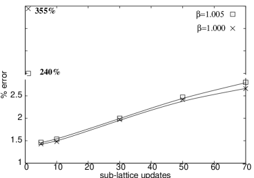
Figure 2: %error on the scalar (top) and axial-vector (bottom) correlator at $\Delta t=2$ after a 10hr. run on a 1.5GHz AMD Athlon PC. $12^{4}$ lattice.

3 Results

In Tables 2 and 2 we present our results for the zero momentum scalar and axial-vector glueball masses.

The (${\vec{k}}\neq 0$) axial-vector correlator is sensitive to a correlation between two 1-forms. In the deconfining region we expect this part to yield information about the photon. Indeed the effective masses from this correlator are very small in the deconfined phase and do not show any variation with $\beta$. To obtain the rest mass, we computed $m^{2}-m^{2}_{k}$ assuming the free field dispersion relation $m^{2}_{k}=\sum_{i}(2-2\cos k_{i})$. Within statistical errors the rest mass turns out to be zero and this we believe is strong evidence for the photon. For a more elaborate discussion of our results see [6].

In Figure 3, we present all the masses along with the region where the phase transition is expected to take place.

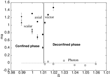
Figure 3: Consolidated plot of glueball masses. $\blacktriangle$ and $\blacktriangledown$ : scalar channel (${\vec{k}}=0$) from $\partial\partial^{*}\langle C\rangle$ and $\partial^{*}\partial\langle C\rangle$. $\bullet$ : axial-vector channel (${\vec{k}}=0$). $\square$ : photon from the axial-vector correlator.

Table 1: Zero momentum scalar glueball masses

$\beta$	$\partial_{t}^{*}\partial_{t_{0}}\langle C(t,t_{0})\rangle$	$\partial_{t}\partial_{t_{0}}^{*}\langle C(t,t_{0})\rangle$
0.990	1.195 (55)	1.085 (50)
1.000	0.875 (41)	0.812 (37)
1.005	0.682 (29)	0.693 (29)
1.010	0.405 (22)	0.410 (21)

Table 2: Zero-momentum axial-vector glueball masses

Confining regime
$\beta$	1.000	1.005	1.010
$ma$	1.31 (1)	1.096 (9)	0.757 (20)
Deconfining regime
$\beta$	1.012	1.015	1.020
$ma$	1.068 (38)	1.279 (24)	1.47 (8)

References

- [1] G. Arnold, T. Lippert, K. Schilling, T. Neuhaus, Nucl. Phys. Proc. Suppl. 94, (2001) 651
- [2] B. Berg, C. Panagiotakopoulos, Phys. Rev. Lett. 52 (1984) 94
- [3] J.D. Stack, R. Filipczyk, Nucl. Phys. Proc. Suppl. 63 (1998) 537
- [4] M. Lüscher, P. Weisz, JHEP 0109 (2001) 010
- [5] H.B.Meyer, JHEP 0301 (2003) 048
- [6] P. Majumdar, Y. Koma, M. Koma, hep-lat/0309003