Kaon B Parameter in Quenched QCD

Abstract

I calculate the kaon B-parameter $B_{K}$, defined via ${8\over 3}(m_{K}f_{K})^{2}B_{K}=\langle\bar{K}|\bar{s}\gamma_{\mu}(1-\gamma_{5})d\bar{s}\gamma_{\mu}(1-\gamma_{5})d|K\rangle$, with a lattice simulation in quenched approximation. The lattice simulation uses an action possessing exact lattice chiral symmetry, an overlap action. Computations are performed at two lattice spacings, about 0.13 and 0.09 fm (parameterized by Wilson gauge action couplings $\beta=5.9$ and 6.1) with nearly the same physical volumes and quark masses. I describe particular potential difficulties which arise due to the use of such a lattice action in finite volume. My results are consistent with other recent lattice determinations using domain-wall fermions.

I Introduction

The kaon B-parameter $B_{K}$, defined as ${8\over 3}(m_{K}f_{K})^{2}B_{K}=\langle\bar{K}|\bar{s}\gamma_{\mu}(1-\gamma_{5})d\bar{s}\gamma_{\mu}(1-\gamma_{5})d|K\rangle$, is an important ingredient in the testing of the unitarity of the Cabibbo-Kobayashi-Maskawa matrix Hocker:2001xe . It has been a target of lattice calculations since the earliest days of numerical simulations of QCD. Lattice calculations of $B_{K}$ require actions with good chiral properties, since the matrix element of the four-fermion operator scales like the square of the pseudoscalar meson mass as that mass vanishes. If the lattice action does not respect chiral symmetry, the desired operator will mix with operators of opposite chirality. The matrix elements of these operators do not vanish at vanishing quark mass, and therefore overwhelm the signal.

There has been a continuous cycle of lattice calculations using fermions with ever better chiral properties. This calculation is yet another incremental upgrade, to the use of a lattice action with exact $SU(N_{f})\otimes SU(N_{f})$ chiral symmetry, an overlap ref:neuberfer action. These actions have operator mixing identical to that of continuum-regulated QCD Capitani:2000da .

The first lattice calculations of $B_{K}$ were done with Wilson-type actions. Techniques for handling operator mixing have improved over the years, (for recent results, see Gupta:1996yt -Aoki:1999gw ) but this approach remains (in the author’s opinion) arduous.

Staggered fermions (Kilcup:1997ye –Aoki:1997nr ) have enough chiral symmetry at nonzero lattice spacing, that operator mixing is not a problem. One can obtain extremely precise values for lattice-regulated $B_{K}$ at any fixed lattice spacing. However, to date, all calculations of $B_{K}$ done with staggered fermions use “unimproved” (thin link, nearest-neighbor-only interactions), and scaling violations are seen to be large. For example, the JLQCD collaboration Aoki:1997nr saw a thirty per cent variation in $B_{K}$ over their range of lattice spacings.

Domain wall fermions pin chiral fermions to a four dimensional brane in a five dimensional world; chiral symmetry is exact as the length of the fifth dimension becomes infinite. For real-world simulations, the fifth dimension is finite and chiral symmetry remains approximate, though much improved in practice compared to Wilson-type fermions. Two groups AliKhan:2001wr ; Blum:2001xb have presented results for $B_{K}$ with domain wall fermions. Ref. AliKhan:2001wr has data at two lattice spacings and sees only small scaling violations. There is a few standard deviation disagreement between the published results of the two groups.

Finally, overlap actions have exact chiral symmetry at finite lattice spacing. All operator mixing is exactly as in the continuum Capitani:2000da . Two groups Garron:2003cb ; DeGrand:2002xe have recently presented results for $B_{K}$ using overlap actions, but the actions and techniques are completely different. The second of these is a preliminary version of the work described here.

The lattice matrix elements must be converted to their continuum-regularized values and run to some fiducial scale. Matching coefficients can be computed perturbatively or nonperturbatively. For most standard discretizations of fermions, the matching factors (“Z-factors”) are quite different from unity. For these actions, perturbation theory is regarded as untrustworthy, and other methods must be employed. I, however, use an action in which the gauge connections are an average of a set of short range paths, specifically HYP-blocked linksref:HYP . Ref. DeGrand:2002va has computed the matching factors for operators relevant for this study, as well as the scale for evaluating the running coupling, using the Lepage-Mackenzie-Hornbostel ref:LM ; Hornbostel:2000ey criterion. The Z-factors are quite close to unity. A number of calculations of Z-factors for related actions Bernard:1999kc reveal that this behavior is generic for actions with similar kinds of gauge connections. In this work I compare perturbative and nonperturbative calculations of two Z-factors, for the local axial current and for the lattice-to- $\overline{MS}$ quark mass matching factor, and find reasonable agreement between them.

Having exact chiral symmetry forces one to confront the problem that this calculation is performed in quenched approximation. These results will not be directly applicable to the real world of QCD with dynamical fermions. I encounter difficulties in two places. First, there is no reason for the spectrum of quenched QCD to be identical to that of full QCD. Using different physical observables to extract a strange quark mass can (and does) lead to different values of this parameter. At small quark masses, my observed $B$ parameter varies strongly with quark mass, and my prediction for $B_{K}$ is sensitive to my choice of $m_{s}$.

The second difficulty is more fundamental. In order to extrapolate results to the chiral limit, one must use chiral perturbation theory. However, the symmetries of quenched QCD are different from the symmetries of full QCD. Not only are the leading coefficients expected to be different in quenched and full QCD, but the logarithmic contributions to any observable $Q$

$$Q(m_{PS})=A(1+B{m_{PS}^{2}\over f_{PS}^{2}}\log m_{PS}^{2})+\dots$$ (1)

can have different coefficients (different $B$’s in Eq. 1), or different functional form (in the formula for $m_{PS}^{2}/m_{q}$, the coefficient of $\log(m_{PS}^{2})$ is not $m_{PS}^{2}$ but a constant related to the quenched topological susceptibility Sharpe:1992ft ; BG ). All of these differences are encountered in the analysis of the data. To produce a prediction for an experimental number using results of a quenched simulation involves uncontrolled, non-lattice-related phenomenological assumptions.

I conclude this introduction by presenting graphs which illustrate my results. Fig. 1 shows results for $B_{K}$ at various lattice spacings, for a selection of simulations which have reasonable statistics and small error bars. Fig. 2 presents results which are either extrapolated to the continuum limit, or presented by their authors as having small lattice spacing artifacts.

Figure 1: $B_{K}$ comparisons vs lattice spacing, from a selection of simulations with reasonably small error bars. Results are labeled diamonds and fancy diamondAoki:1997nr , the fancy cross Garron:2003cb , octagons AliKhan:2001wr , the cross Blum:2001xb , and squares (this work).

Figure 2: $B_{K}$ comparisons presented “as if” they were taken to the continuum limit. The label in parentheses characterizes the kind of lattice fermions used: W for Wilson, Cl for Clover, KS for staggered, DW for domain wall, and OV for overlap fermions. References are GBS Gupta:1996yt , JLQCD(W) Aoki:1999gw , Conti Conti:1997qk , KGS Kilcup:1997ye , JLQCD(KS) Aoki:1997nr , CP-PACS AliKhan:2001wr , RBC Blum:2001xb , GGHLR Garron:2003cb , and MILC, this work. The points of Refs. Aoki:1999gw , Kilcup:1997ye , Aoki:1997nr , AliKhan:2001wr , and this work are the results of a a continuum extrapolation; all the rest are simulations at one lattice spacing.

In Section 2 I describe the action, simulation parameters, and data sets. Sec. 3 is devoted to a discussion of zero mode effects and my attempts to deal with them. Results relevant to $B_{K}$ are presented in Sec. 4. In Sec. 5 I discuss the chiral limit of $B_{K}$ and of operators $O_{7}^{3/2}$ and $O_{8}^{3/2}$, relevant for part of $\epsilon^{\prime}/\epsilon$. My brief conclusions are given in Sec. 6. An Appendix compares perturbative and nonperturbative matching factors.

II Simulation techniques

II.1 Data sets

The data set used in this study is generated in the quenched approximation using the Wilson gauge action at couplings $\beta=5.9$ (on a $12^{3}\times 36$ site lattice), where I have an 80 lattice data set, and $\beta=6.1$ (on a $16^{3}\times 48$ site lattice) with 60 lattices. The nominal lattice spacings are $a=0.13$ fm and 0.09 fm from the measured rho mass. Propagators for ten ($\beta=5.9$) or nine ($\beta=6.1$) quark masses are constructed corresponding to pseudoscalar-to-vector meson mass ratios of $m_{PS}/m_{V}$ ranging from 0.4 to 0.85. The fermions have periodic boundary conditions in the spatial directions and anti-periodic temporal boundary conditions. I gauge fix to Coulomb gauge and take our sources to be Gaussians of size $x_{0}/a=3$, 4.125 at $\beta=5.9$, 6.1 (where the quark source is $\Phi=\exp(-x^{2}/x_{0}^{2})$).

II.2 Lattice action and simulation methodology

The massless overlap Dirac operator is

$$D(0)=x_{0}(1+{z\over{\sqrt{z^{\dagger}z}}})$$ (2)

where $z=d(-x_{0})/x_{0}=(d-x_{0})/x_{0}$ and $d(m)=d+m$ is a massive “kernel” Dirac operator for mass $m$. The massive overlap Dirac operator is conventionally defined to be

$$D(m_{q})=({1-{m_{q}\over{2x_{0}}}})D(0)+m_{q}$$ (3)

and it is also conventional to define the propagator so that the chiral modes at $\lambda=2x_{0}$ are projected out,

$$\hat{D}^{-1}(m_{q})={1\over{1-m_{q}/(2x_{0})}}(D^{-1}(m_{q})-{1\over{2x_{0}}}).$$ (4)

This also converts local currents into order $a^{2}$ improved operators Capitani:1999uz .

The overlap action used in these studiesref:TOM_OVER is built from a kernel action with nearest and next-nearest neighbor couplings, and HYP-blocked linksref:HYP . HYP links fatten the gauge links without extending gauge-field-fermion couplings beyond a single hypercube. This improves the kernel’s chiral properties without compromising locality.

The “step function” ($\epsilon(z)=z/\sqrt{z^{\dagger}z}$) is evaluated using the fourteenth-order Remes algorithm of Ref. ref:FSU (after removing the lowest 20 eigenmodes of $z^{\dagger}z$). This involves an inner (multimass ref:multimass ) conjugate gradient inversion step. It is convenient to monitor the norm of the step function $|\epsilon(z)\psi|^{2}/|\psi|^{2}$ and adjust the conjugate gradient residue to produce a desired accuracy (typically $10^{-5}$ in $\epsilon(z)\psi$). Doing so, I need about 16-18 inner conjugate gradient steps at $\beta=5.9$ and 10-12 steps at $\beta=6.1$.

An important ingredient of this overlap program has been to precondition the quark propagator by projecting low eigenfunctions of the Dirac operator out of the source and including them exactly. This can in principle eliminate critical slowing down from the iterative calculation of the inversion of the Dirac operator. Of course, there is a cost: one must find the eigenmodes. My impression from the literature, plus my own experience, is that for the overlap with Wilson action kernel, this cost is prohibitive. However, my kernel action is designed to resemble the exact overlap well enough that its eigenvectors are good “seeds” for a calculation of eigenvectors of the exact action, and it is kept simple enough that finding its own eigenvectors is inexpensive.

As a rough figure of merit, consider the $12^{3}\times 36$, $\beta=5.9$ data set. Computing the lowest twenty eigenmodes of the squared massless overlap Dirac operator takes about 8 time units, while the complete set of quark propagators from the lightest mass I studied to the heaviest takes about 16 time units times two (for two sets of propagators) per lattice. Fig. 3 shows the number of conjugate gradient steps needed to compute the quark propagator to some fixed accuracy, as a function of bare quark mass. If one would naively extrapolate the heavy quark results (for which low eigenmodes make only a small contribution) to lower masses, one would see a forty per cent reduction in the number of inverter steps needed at the smallest quark mass, vs an additional cost of 8/32 = 25 per cent per propagator set for the construction of eigenmodes.

Figure 3: Number of conjugate gradient steps in the calculation of quark propagators, as a function of quark mass. The four curves are two different sources on each of two different lattices, and we are converging to a fractional accuracy of the squared residue of $10^{-14}$ for this test case.

II.3 Correlation functions

The “generic” four fermion operator one must consider is

$$O=(\bar{q}^{(1)}_{\alpha}\Gamma_{1}q^{(2)}_{\beta})\otimes(\bar{q}^{(3)}_{\gamma}\Gamma_{2}\hat{q}^{(4)}_{\delta})$$ (5)

(the superscript labels flavor; the subscript, color). Special cases are (a) $O=O_{1}$: $\Gamma_{1}=\Gamma_{2}=\gamma_{\mu}(1-\gamma_{5})$, $\alpha=\delta$, $\beta=\gamma$; (b) $O=O_{2}$: $\Gamma_{1}=\Gamma_{2}=\gamma_{\mu}(1-\gamma_{5})$, $\alpha=\beta$, $\gamma=\delta$; and (c) the isospin 3/2 operators for electroweak penguins, here written with the normalization conventions used in Refs. Blum:2001xb and Noaki:2001un

$$O_{7}^{3/2}={1\over 2}\big{(}(\bar{s}_{\alpha}\gamma_{\mu}(1-\gamma_{5})d_{\alpha})[(\bar{u}_{\beta}\gamma_{\mu}(1+\gamma_{5})u_{\beta})-(\bar{d}_{\beta}\gamma_{\mu}(1+\gamma_{5})d_{\beta})]+(\bar{s}_{\alpha}\gamma_{\mu}(1-\gamma_{5})u_{\alpha})(\bar{u}_{\beta}\gamma_{\mu}(1+\gamma_{5})d_{\beta})\big{)}$$ (6)

and

$$O_{8}^{3/2}={1\over 2}\big{(}(\bar{s}_{\alpha}\gamma_{\mu}(1-\gamma_{5})d_{\beta})[(\bar{u}_{\beta}\gamma_{\mu}(1+\gamma_{5})u_{\alpha})-(\bar{d}_{\beta}\gamma_{\mu}(1+\gamma_{5})d_{\alpha})]+(\bar{s}_{\alpha}\gamma_{\mu}(1-\gamma_{5})u_{\beta})(\bar{u}_{\beta}\gamma_{\mu}(1+\gamma_{5})d_{\alpha})\big{)}.$$ (7)

$B_{K}$ is proportional to the matrix element of $O_{+}=O_{1}+O_{2}$. Because overlap fermions are chiral, one can extract $B_{K}$ from the matrix element of the operator between zero momentum states. All the operators to be studied have only “figure-eight” topology matrix elements, where each field in the operator contracts against a field in the source or sink interpolating field. There are no penguin graphs (where fields in the operator contract against each other) as long as one works in the degenerate-mass limit.

Broadly speaking, the matrix element of a four-fermion operator is computed by placing interpolating fields for a meson at two widely-separated locations on the lattice and contracting field variables between these sources and the operator, to construct an un-amputated correlator containing the operator. There are two commonly-used strategies for doing this: One possibility is to build all the quark propagators “at the operator” at one location on the lattice, and to join up pairs of propagators to make the mesons. The second method is to construct propagators from two well-separated sources and bring them together at the operator. The advantages of the first method are that one needs half as many propagators per lattice, and it is possible to project the whole calculation into a particular momentum eigenstate (by appropriately summing over locations of the meson interpolating fields). The major disadvantage of this method is that one is only measuring the matrix element of the operator at one location per propagator construction. With the second method one can average the location of the operator over all spatial and many temporal locations, a considerable gain in statistics. A disadvantage of the second method is that unless the source generates a hadronic state which is a momentum eigenstate the correlator will involve a mixture of the eigenstates. The dominant contribution to the correlator is from $\vec{p}=0$, but there will be a contamination from higher momentum states. I have chosen the second method, and will discuss below how I dealt with higher-momentum modes. I placed the two source time slices $N_{t}/2-2$ temporal sites apart; with the toroidal geometry there are two temporal regions where the operator is “between” the sources. I combine all two-point function data sets from the two sources in the fits.

The correlator of two interpolating fields located at $x,t=(0,0)$ and $(0,T)$ with an operator $S(x,t)$ summed over $x$ is then

$$C_{3}(t,T)=\sum_{x}\langle\Phi(0,T)S(x,t)\Phi(0,0)\rangle$$ (8)

Inserting complete sets of relativistically normalized momentum eigenstates, and assuming $\langle h(\vec{p}_{1})|S(\vec{p})|h(\vec{p}_{2})\rangle$ is proportional to $\delta(\vec{p}+\vec{p}_{2}-\vec{p}_{1})$,

$$C_{3}(t,T)=\sum_{\vec{p}}\exp(-E(\vec{p})T)\langle 0|\Phi|h(\vec{p})\rangle|^{2}{1\over{(2E(\vec{p}))^{2}}}{1\over V}\langle h(\vec{p})|S|h(\vec{p})\rangle.$$ (9)

If the $\vec{p}=0$ state dominates the sum,

$$C_{3}(t,T)=\exp(-mT)|\langle 0|\Phi|h\rangle|^{2}{1\over{(2m)^{2}}}{1\over V}\langle h|S|h\rangle.$$ (10)

However, “dominance in the sum” is controlled by the quantity $\exp((-E(\vec{p})-m)T)$. These sources do not make momentum eigenstates, and so the $\vec{p}=0$ $B_{K}$ signal is contaminated by a $\vec{p}\neq 0$ contribution. The minimum momentum in a finite box of side $L$ is $|p|=2\pi/L$. Because of the small masses involved, the contamination is not present at quark masses below 2-3 times the strange quark mass. It appears at bigger quark mass, because $E(\vec{p})-m$ gets smaller as the pseudoscalar mass $m$ grows. Fortunately, there are two inequivalent paths on the torus to disentangle the two “signals,” and one can fit the $B_{K}$ correlator to a sum of a $\vec{p}=0$ term and a $p=2\pi/L$ term.

II.4 Fitting and Error Analysis

In a Monte Carlo simulation different quantities measured on the same set of lattices are highly correlated, and it is preferable to analyze the data using covariant fits. However, in order to determine accurately the small eigenvalues of the correlation matrix, large statistical samples are needed. If the statistical sample is too small, these eigenvalues can be poorly determined, and the fits will become unstable. This can be a particular problem in fits which extract $B_{K}$, simply because they can involve many degrees of freedom (one three-point function and up to two two-point functions). My solution to this problem is to adopt the strategy of the analysis used in Ref. Bernard:2002pc . I compute the correlation matrix (the covariance matrix, but normalized by the standard deviation so that its diagonal entries are the identity), and find its eigenvalues and eigenvectors. I then reconstruct the matrix, discarding eigenvectors whose eigenvalues are smaller than some cutoff. This matrix is singular, so I reset the values of its diagonal entries to the identity again. I use this processed covariance matrix as an input to the fit.

This is basically the strategy adopted in Ref. Bernard:2002pc , except that here the cut on kept eigenvectors is chosen to be a fraction of the largest eigenvector, rather than a fixed value. I have taken the value of this cutoff to be 0.1, and have varied it to insure that fits are insensitive to it.

(My experience in this work is that all fits to spectroscopic quantities, and fits to pairs of two point function, used, for example, to extract pseudoscalar decay constants, produce statistically identical results regardless of the number of eigenvalues discarded.)

All chiral extrapolations of data are done by performing correlated fits to extract necessary physical parameters quark mass by quark mass, then performing extrapolations under a single-elimination jackknife.

I have performed a number of different analyses of the data. Fits of the three point function with a particular sources (pseudoscalar or axial vector, labeled PS or A) can be combined with two-point functions with axial vector sinks to give the B-parameters directly,

$$C_{3}(t,T)={8\over 3}{{Z^{2}}\over{V}}(B\exp(-mT)+C_{1}\exp(-E(p)T))$$ (11)

($E(p)^{2}=m^{2}+(2\pi/L)^{2}$ is the energy of the lowest nonzero momentum state) and

$$C_{2}(t,t^{\prime})=Z(\exp(-m(t-t^{\prime})-\exp(-m(N_{t}-(t-t^{\prime})).$$ (12)

This is done by performing a correlated fit with three ($Z$, $B$, $m_{PS}$) or four (add $C_{1}$) parameters to $C_{3}(t,T)$, $C_{2}(t,0)$, and $C_{2}(t,T)$.

As a check, one can also simply perform a (jackknife-averaged) fit of the ratio $C_{3}(t,T)/[C_{2}(t,0)C_{2}(t,T)]$ to a constant. The range of $t$ is varied with a search for plateaus in the fit value. This method has been commonly used in many previous measurements of $B$ parameters. When I compare this “ratio” fit to a full correlated fit to $B_{K}$, I always find consistency of the fitted $B$ parameter. Generally, the error bar assigned to it by the ratio fit is about forty percent ot the size of the uncertainty of the correlated fit. However, I elect NOT to use these more optimistic estimations of the uncertainty because they do not attempt to include any of the correlations which are known to be present in the data.

One can also extract the matrix element of the operator by doing a correlated fit of $C_{3}(t,T)$ for a particular source and a two-point function which uses the same source as a sink. In this case

$$C_{3}(t,T)={{Z^{\prime}}\over{(2m)^{2}V}}(\langle O\rangle\exp(-mT)+C^{\prime}_{1}\exp(-E(p)T))$$ (13)

and

$$C_{2}(t,t^{\prime})={{Z^{\prime}}\over{2m}}(\exp(-m(t-t^{\prime})+\exp(-m(T-(t-t^{\prime})).$$ (14)

With these correlators, the B parameter can be extracted by doing a simultaneous fit to another correlator set, which gives $f_{PS}$ and $m_{PS}$, and jackknife averaging. This increases the resulting uncertainty in $B_{K}$, so this method is not competitive with the three-propagator fits.

At lower quark mass the size of the $\vec{p}\neq 0$ contamination falls to zero. Fits which include the $C_{1}$ coefficient become unstable, because the fit is completely insensitive to it. The Hessian matrix develops a near-zero eigenvalue as a result of this insensitivity. Usually, this near zero mode just means that the $C_{1}$ coefficient will be poorly determined, but a zero mode in a Hessian matrix is always dangerous, and can corrupt the whole fit. To determine the minimum quark mass where $C_{1}$ is not needed, I performed fits where the inversion of the covariance matrix was done using singular value decomposition (clipping out eigenmodes with eigenmodes smaller than some minimum cut). I varied the ratio of smallest to largest eigenvalues kept in the $4\times 4$ Hessian matrix. Any “reasonable” choice (conditioning number cut $\geq 10^{-5}$) stabilizes the inversion by decoupling and freezing out any variation in $C_{1}$.

III Zero mode effects

Simulations with lattice fermions possessing an exact chiral symmetry done in finite volume have a “new” kind of finite volume artifact: the presence of exact zero modes of the Dirac operator, through which quarks can propagate. In some cases (the eta prime channel, for example) the zero modes contribute physics, but for the case of $B_{K}$ they are merely an annoyance which would disappear in the infinite volume limit.

Things could be much worse. For example, for Wilson-type fermions the analogs of zero modes are configurations where the Dirac operator has real eigenvalues. Because these theories are not chiral, eigenvalues of the massless Dirac operator $D$ are not “protected”– they can take on any real value. It can happen that this real value coincides with the negative of the simulation mass $m$. Then $D+m$ is simply non-invertible. Typically, these eigenmodes occur at small quark mass, meaning that it is difficult (if not impossible) to do simulations there.

Note that zero modes will also be present in simulations with nonzero mass dynamical fermions, although their effects are likely to be less severe; the dynamical fermions suppress zero modes but (except at zero quark mass) do not eliminate them.

There are basically five observables needed in a $B_{K}$ calculation.

• The pseudoscalar mass

• The vector meson mass (to set the lattice spacing)

• The matrix element of $O_{+}$

• The matrix element of the axial vector current

• The pseudoscalar decay constant

All can (in principle) be affected by finite volume zero modes artifacts at small quark mass.

The most obvious way to check for finite volume effects is to do simulations at several volumes. I did not do that. One could use sources which do not couple to zero modes. This is the strategy pursued by Ref. Garron:2003cb : their meson interpolating fields are the linear combination $\gamma_{0}\gamma_{5}-\gamma_{0}$. I did not do that either. The $\gamma_{0}$ part of the source couples only to the (heavy) scalar meson, not to the pseudoscalar meson. Its contribution to the pseudoscalar meson matrix element of the operator averages to zero but contributes noise in a finite data set. Because of the PCAC relation, the $\gamma_{0}\gamma_{5}$ source decouples for the pseudoscalar meson in the chiral limit, so that while one is decoupling zero modes, we are also decoupling from the desired channel.

Instead, I used the fact that zero mode effects are different in different channels. I measured the same physical observable using different operators (presumably with different zero mode contributions) and looked for differences.

When one fits correlators to extract pseudoscalar masses, one can perform the fits naively, without consideration of the zero modes. Then if zero modes are present in some channels, observables such as the pseudoscalar mass inferred from these channels will show characteristic differences. As the zero mode correlator reflects some underlying structure of the gauge field responsible for configurations which support zero modes, it produces correlations on a scale which is independent of the quark mass. Thus, a plot of $m_{PS}^{2}/m_{q}$ would diverge at small $m_{q}$ inversely with $m_{q}$ (simply because $m_{PS}$ would be independent of $m_{q}$). I searched for this suspicious behavior in plots of $m_{PS}^{2}/m_{q}$ vs $m_{q}$ (Fig. (4). Correlators include the pseudoscalar current (which has a contribution from the propagation of both quarks through zero modes), the pseudoscalar-scalar difference (in which all zero mode contributions cancel), and the axial current correlator (which has a “mixed” contribution with one quark propagating through zero modes and the other through nonzero modes: this contribution in independent of $m_{q}$ at small $m_{q}$.) Within statistical uncertainties, I do not see any difference between these channels. I anticipate that this would not be the case at smaller quark mass or smaller volumes. Nevertheless, on theoretical grounds I elect to only extract pseudoscalar masses at small quark masses from the pseudoscalar-scalar difference.

Figure 4: (a) $\beta=5.9$ and (b) $\beta=6.1$: $(am_{PS})^{2}/(am_{q})$ vs $am_{q}$ from pseudoscalar (crosses), axial vector (octagons) and pseudoscalar-scalar difference (diamonds) sources.

At larger quark mass the pseudoscalar-scalar difference degrades as a pseudoscalar source, compared to pseudoscalar or axial currents. The window of timeslices in which the fitted mass is stable shrinks. Presumably what is happening is that the heavier pseudoscalar feels the effect of the scalar meson (with which it would become degenerate in the heavy quark limit). This effect has been noted by Ref. Gattringer:2002sb .

Note (parenthetically) that the data strongly hint at the presence of an increase in $m_{PS}^{2}/m_{q}$ at small $m_{q}$ which is consistent with a quenched chiral logarithm. The data set is not optimized to precisely pin down these effects (the smallest quark mass is still rather large). In an attempt to look for these terms, I have fit $m_{\pi}^{2}/m_{q}$ to two functional forms: The first one is Sharpe:1992ft ; BG :

$$(am_{PS})^{2}/(am_{q})=A[1-\delta(\ln(Am_{q}/\Lambda)+1)]+B(am_{q})$$ (15)

It contains three free parameters, $A$, $B$, and $\delta$, as well as the scale for the chiral logarithm, $\Lambda$, which I do not let float in the fit but instead pin to any of several fiducial values between 0.8 and 1.2 GeV.

The second functional form is due to Sharpe Sharpe:1992ft :

$$(am_{PS})^{2}/(am_{q})=C(am_{q})^{(\delta/(1+\delta)}+D(am_{q})$$ (16)

I elect to perform fits to a mix of pseudoscalar-scalar difference correlators at low quark mass and axial correlators at high mass (rejecting the pure pseudoscalars on theoretical grounds). I saw little shift in the fitted $\delta$ as I varied $\Lambda$, and the fits give $\delta=0.17(5)$ at $\beta=5.9$, 0.20(7) at $\beta=6.1$. The power law fit gives $\delta=0.18(5)$ at $\beta=5.9$ and $0.21(9)$ at $\beta=6.1$. (All chiral extrapolations from the $\beta=6.1$ data set are noisier than their $\beta=5.9$ counterparts because the former set does not extend to as low a value of the quark mass.)

Recent determinations of $\delta$ from a variety of actions show quite wide spread (for a recent review, see Wittig:2002ux ). I am very much aware that my results have uninterestingly large error bars compared to the recent high-statistics, low pseudoscalar mass results of Ref. Dong:2003im . My purpose in quoting them here is to illustrate that I see behavior in the data which is consistent with the expectations of quenched QCD, and inconsistent with the expectations of full QCD. The choices for the quark mass relevant to the kaon will occur in the rise near the minimum of the $m_{PS}^{2}/m_{q}$ vs $m_{q}$ plot.

These results are quite a bit greater than ones reported by Heller and me DeGrand:2002gm , using an overlap action with the same fermion kernel, but with gauge connections which are much more smoothed than the ones used in this study. Presumably the smaller value for $\delta$ seen there came about because the additional smoothing suppressed the coupling of the fermions to smaller topological objects.

The vector meson mass is shown as a function of the quark mass (both in lattice units) in Fig. 5). It was measured with the correlator of two vector currents. It is expected to have only an “interference term” like the axial vector correlator. As the quality of the signal degrades at low quark mass, and as I only use vector masses at larger quark masses, or use all masses to make linear extrapolations to the chiral limit, I will not investigate this data set further.

Figure 5: $am_{V}$ vs $am_{q}$, (a) $\beta=5.9$, (b) $\beta=6.1$.

The pseudoscalar decay constant, defined through $f_{PS}=m_{PS}^{2}/(2m_{q})\langle 0|\bar{\psi}\gamma_{5}\psi|PS\rangle$, is shown in Fig. 6. It is extracted it from a correlated fit to a two-point function with Gaussian source and sink and one with a Gaussian source and local pseudoscalar current sink. I have used pseudoscalar and axial sources, as well as a fit where the two correlators are the pseudoscalar-scalar difference. There is some tendency for the latter correlators to produce a smaller decay constant at smaller quark mass and a larger one at larger quark mass. The deviation of the decay constant measured using pseudoscalar sources and sinks from that measured in other channels at lower quark mass may reflect the effects of zero modes in that channel (it is consistent with previous work byGiusti:2001pk ). The deviation of the quantity measured in the pseudoscalar-scalar difference channel at larger quark mass is almost certainly due to the degradation in the signal from the difference correlator there: the fit simultaneously produces the pseudoscalar mass along with the decay constant, and this mass also drifts away from that of the other channels.

When $(af_{PS})$is needed below, I will use the pseudoscalar-scalar difference at low quark mass and the axial source correlators at higher mass, and vary the crossover mass to make sure that the results are not sensitive to it.

Figure 6: (a) $(af_{PS})$ vs $m_{q}$, (a) $\beta=5.9$, (b) $\beta=6.1$. The labels crosses, squares, and diamonds label decay constants extracted from pseudoscalar correlators, differences of pseudoscalar and scalar correlators, and correlators with axial sources. (c), (d): The small mass region of panels (a), (b) magnified.

Finally, there are the operators contributing to $B_{K}$ itself. I performed correlated fits of three and two point functions (Eqs. 13 and 14) to extract the matrix element of $O_{+}$. I considered two cases: pseudoscalar sources for the three point function, and the pseudoscalar - scalar difference for the two point function, and fits to correlators where all interpolating fields are axial currents. Differences in the fits under variation in the ranges are comparable to the error bars shown. I also investigated fits to the axial vector current operator, using source interpolating fields which were either pseudoscalar or axial vector. An example of such a search is shown in Fig. (7). Only at the smallest mass, not at the kaon, does the operator appear to be affected. Thus the extraction of the $B$ parameter in the chiral limit might be compromised by finite volume effects, but not $B_{K}$ itself.

Figure 7: Three parameter correlated fits extracting the matrix element $\langle O_{+}\rangle$ from a correlator of the operator and a two point function. (a) $\beta=5.9$, (b), $\beta=6.1$. Meson interpolating fields are squares for pseudoscalar-scalar difference source and octagons for the axial vector source for both correlation functions. The “denominator” of $B_{K}$ can be checked by extracting the axial vector current matrix element $m_{PS}f^{A}_{PS}$ from a correlated fit of two point functions; this is shown in (c) and (d) for $\beta=5.9$ and 6.1. Here crosses show the pseudoscalar-axial vector correlator and octagons from the difference of $(\gamma_{0}\gamma_{5}-\gamma_{0}\gamma_{5})$ and $(\gamma_{0}-\gamma_{0})$ correlators, which has no zero modes.

IV Data analysis for $B_{K}$

IV.1 Fits to Lattice $B_{K}$

$B_{K}$ can be extracted from covariant fits or ratios of three propagators. A typical correlated fit of the figure-eight graph and two axial vector sink correlators, and a ratio plot are is shown in Fig. 8. Correlated fits are stable against variations in fit ranges or cuts on the correlation matrix and have reasonable confidence levels. Uncorrelated jackknife “ratio fits” are consistent with the correlated fits, have small uncertainties and are also quite stable over a wide range of time slices. Examples of these extractions are shown in Figs. 9, 10 and 11. My results for the B-parameter in lattice regularization as a function of the bare quark mass are shown in Tables 1 and 2.

Figure 8: Examples of data sets, $\beta=5.9$, $am_{q}=0.035$, PS sources. (a) Correlators from which $B_{K}$ is fit, with solid lines showing the fit. Correlators 1 and 2 (crosses and octagons) have pseudoscalar sources and axial vector sinks; correlator 3 (diamonds) is the figure-eight graph. (b) Ratio of correlators from which $B_{K}$ is fit.

Figure 9: $B_{K}$ extracted from (a) correlated fits to three propagators and (b) jackknifed ratios of propagators, with pseudoscalar sources, $\beta=5.9$. Fits are over the range $t=6-10$, 24-28. In (a), squares show three-parameter fits and crosses show four-parameter fits, while in (b) the squares are from fits of the ratio to a constant, while the crosses include the lowest $\vec{p}\neq 0$ contribution.

Figure 10: $B_{K}$ extracted from (a) correlated fits to three propagators and (b) jackknifed ratios of propagators, with pseudoscalar sources, $\beta=6.1$. sources, $\beta=5.9$. Fits are over the range $t=8-14$, 30-38. Labels are as in Fig. 9.

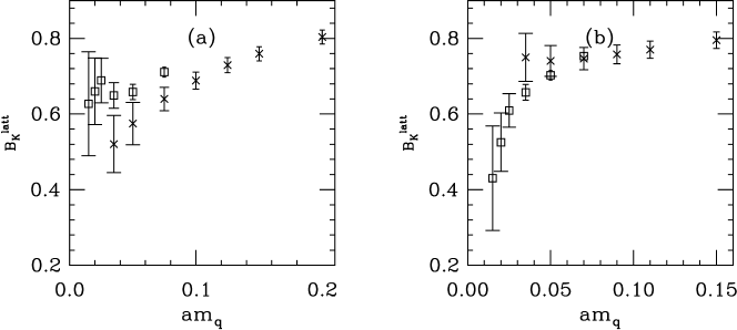
Figure 11: $B_{K}$ extracted from jackknife averages of ratios of correlators, with axial vector sources, (a) $\beta=5.9$, (b) $\beta=6.1$. Squares show constant-ratio fits and crosses show fits keeping the $\vec{p}\neq 0$ term.

IV.2 Matching Factors

The naive dimensional regularization (NDR) $B_{K}$ at a scale $\mu$ is related to the lattice-regulated number (from lattice scale $a$) by

$$B_{K}^{(NDR)}(\mu)=RB_{K}^{(latt)}={{Z_{TOT}(\mu,a)}\over Z_{A}^{2}}B_{K}^{(latt)}$$ (17)

where the conversion factor for the operator $O_{+}$, $Z_{TOT}$, can be decomposed into

$$Z_{TOT}(\mu,a)=Z_{NDR}(\mu,m)Z_{PT}(ma,qa).$$ (18)

$Z_{A}$ is the axial current matching factor. $Z_{NDR}(\mu,a)$ is the usual two-loop running formula for the NDR operator, carrying it from scale $m$ to scale $\mu$. $Z_{PT}(ma,qa)$ is the lattice-to-NDR matching factor connecting lattice scale $a$ with continuum scale $m$,

$$Z_{PT}(ma,qa)=1+{{g^{2}(qa)}\over{16\pi^{2}}}[-\gamma_{0}\ln{ma}+b]$$ (19)

$\gamma_{0}$ is the anomalous dimension of the operator; $b$ is the lattice-action-dependent matching term ($b=-3.98$ for the action used here DeGrand:2002va ). One can imagine several different choices for the product of $Z$’s.

• $ma=1$, $q=q^{*}$ as defined by the Lepage-Mackenzie matching condition ref:LM . I will call this“type 1.”

• Gupta, Bhattacharya, and SharpeGupta:1996yt suggest two versions of “horizontal matching,” where $m=q_{i}$, $q^{*}=q_{i}$. and $q_{i}a=1$ (type 2) or $\pi$ (type 3).

The RGI (renormalization group invariant) $\hat{B}_{K}$ is computed from the NDR B-parameter in the usual way, and I will write the constant which renormalizes the lattice number as $\hat{B}_{K}=\hat{R}B_{K}^{(latt)}$.

I determine the strong coupling constant (in the so-called $\alpha_{V}$ prescription) at a scale $q=3.41/a$ from the plaquette, convert it to $\overline{MS}$ prescription, and run it to the desired scale using the two-loop evolution equation. (In all cases I determine $Z_{A}$ perturbatively, 0.988 at $\beta=5.9$, 0.990 at 6.1.) At $\beta=5.9$ the “type 1” Z-factor is $R=0.97$ and the type 2 choices are 1.00 and 0.95. The conversion factors to the RGI $\hat{B}$ are 1.35, 1.40, 1.31 for the three choices. The $\beta=6.1$ numbers are almost equal: for $B_{K}^{(NDR)}(\mu=2$ GeV), 0.98, 1.01,0.97 and for $\hat{B}$, 1.38, 1.42, 1.36. It appears that a reasonable choice and uncertainty for $R$ is 0.97(3) at $\beta=5.9$ and 0.98(3) at 6.1. (Note that in an extrapolation to the continuum, the same choice for matching convention must be used at all lattice spacings.)

IV.3 “Quenched phenomenology” and the strange quark mass

$B_{K}$ comes from a meson made of two degenerate quarks with a common mass which is the average of the nonstrange and strange quark mass. Unfortunately, if quenched spectroscopy is different from the spectroscopy of full QCD, there is no unique choice for this quark mass, even in the absence of discretizaton-induced scale violations. What follows is a discussion which lies outside the realm of lattice calculations, as I try to motivate some choices for lattice spacings and quark masses over others. Unfortunately, Figs 9-10 show a rather large dependence of the $B$ parameter on the quark mass at small quark mass, so the choice of mass is important phenomenologically.

One choice would be to take the lattice spacing from the Sommer parameter (using the interpolation formula of Ref. ref:precis ) and to set the pseudoscalar mass at the kaon. Either interpolation or a quadratic fit to the pseudoscalar mass $m_{PS}^{2}=dm_{q}$ to $m_{K}r_{0}=1.256$ gives $am_{s}/2=0.027(1)$ at $\beta=5.9$, 0.019(1) at 6.1. (The reader might recall that the interpolation formula of Ref. ref:precis plus a nominal value of $r_{0}=0.5$ fm implies that $a$ would be 0.11 or 0.08 fm at $\beta=5.9$ or 6.1.)

However, setting the lattice spacing from $r_{0}$ will push the predictions for other physical quantities away from experiment. For example, one can extrapolate the vector meson mass, the pseudoscalar decay constant, and their ratio, into zero quark mass. (Both extrapolations are linear in $m_{q}$; in contrast to full QCD, the quenched decay constant has a vanishing chiral logarithm.) A jackknife extrapolation of $f_{PS}/m_{\rho}$ gives 0.166(6) at $\beta=5.9$ and 0.169(8) at $\beta=6.1$, quite close to the physical value of (132 MeV)/(770 MeV)=0.17. Separate extrapolations of $m_{V}$ and $f_{PS}$ to zero quark mass would combine with the Sommer parameter to produce too small values of the rho mass or pseudoscalar decay constants: jackknife extrapolations of the former quantity give $am_{\rho}=0.51(2)$ at $\beta=5.9$ and 0.35(1)) at $\beta=6.1$, while $af_{PS}=0.084(2)$ or 0.060(2). This means that a better match to non-$B_{K}$ phenomenology requires using either $f_{\pi}$ or $m_{\rho}$ to set the scale.

I tried a variety of fits and dimensionless ratios to find a quark mass for the kaon. Two choices which produce similar (but not identical) values are (1) Take the lattice spacing from the rho mass; interpolate or fit $m_{PS}^{2}$ vs $m_{q}$ over a range of quark masses around the kaon to the kaon mass. (2) Simultaneously determine $a$ and $m_{s}$ from the phi meson (assume linear variation of the vector meson mass on the quark mass and the “strange eta” $\bar{s}s$ meson: $m_{\eta_{s}}^{2}+m_{\pi}^{2}=2m_{K}^{2}$); then shift the quark mass: ($m_{s}+m_{ns})/m_{s}=2m_{K}^{2}/m_{\eta_{s}}^{2}$. Both fits are taken over a range of quark masses between $1/2m_{s}$ and $3/2m_{s}$. One can substitute polynomial interpolation for fitting with no change in the resulting quark mass. The first choice gives $am_{q}=0.035(2)$ at $\beta=5.9$, 0.025(2) at $\beta=6.1$; the second choice, $am_{q}=0.029(2)$ at $\beta=5.9$, 0.023(2) at $\beta=6.1$. The values of the $\mu=2$ GeV $\overline{MS}$ strange quark masses from these two choices 110(10) or 92(10) MeV at $\beta=5.9$ and 112(7) or 104(8) MeV at $\beta=6.1$. There is no way to determine if the difference in these numbers is statistical or a quenching systematic.

A comparison of $B_{K}^{NDR}(\mu=2$ GeV) as a function of the pseudoscalar mass in units of the kaon mass for this choice of quark mass ($(m_{PS}/m_{K})^{2}=m_{q}/((m_{s}+m_{d})/2)$) is shown in Fig. 12. The two data sets appear to scale reasonably well.

Figure 12: $B_{K}^{NDR}(\mu=2$ GeV) as a function of quark mass from the two data sets–diamonds for $\beta=5.9$, squares for $\beta=6.1$. The matching factor uses the Lepage-Mackenzie convention and the quark mass comes from a combined fit to the $\phi$ and $\bar{s}s$ pseudoscalar.

In practice, I perform the interpolation of the B-parameter to the kaon under the same jackknife as the determination of the strange quark mass. Both determinations have a statistical uncertainty, and the jackknife attempts to include their correlations. I tried two methods of interpolation: I fit the data of the lowest five quark masses to the chiral logarithm form (Eq. 20, below) or just did a simple polynomial interpolation. Both results agree within uncertainties, although at $\beta=6.1$ the results of the chiral fit produce unacceptably large uncertainties because the chiral parameters are poorly determined. I will use the interpolated values.

To be definite, make choice (2) for the quark mass and take the Lepage-Mackenzie choice for the $Z$-factor. In that case, one will have $B_{K}^{NDR}(\mu=2$ GeV)$=0.540(25)$ at $\beta=5.9$, 0.546(36) at $\beta=6.1$. They lie a bit lower than the staggered JLQCD resultAoki:1997nr or the other overlap calculation of Garron, et alGarron:2003cb , but bracket the two domain wall results of Refs. AliKhan:2001wr and Blum:2001xb . The alternative “choice (1) quark mass” would give $B_{K}=0.563(23)$, 0.552(28) for the two couplings,

Recall that Ref. Blum:2001xb sets $a$ from the rho mass and chooses the bare quark mass to put $m_{K}$ at “its physical mass” while Ref. AliKhan:2001wr sets the strange quark mass “from the experimental value of $m_{K}/m_{\rho}$.” My neglect of $r_{0}$ as compared to hadronic masses is at least consistent with the choice of groups with which I want to compare. (Of course, that does not make it correct.) Oddly enough, the “choice 1 mass” which gives us a larger $B_{K}$ is more like the RBC convention (and their value for $B_{K}$ is below mine), and the “choice 2 quark mass” which gives a lower mass is more like that of Ref. AliKhan:2001wr , which lies above my data. Perhaps I am just being obsessive about one standard deviation effects.

Although they show no scaling violations, an extrapolation of the “type 2 mass” results to zero lattice spacing $B(a)=B_{0}+a^{2}B_{1}$ would give a continuum prediction of $B_{K}=0.550(67)$ for this choice of quark mass and matching factor. (The RGI $\hat{B}_{K}$ would be 0.751(35) at 5.9, 0.769(51) at 6.1 and 0.781(94) for an extrapolated continuum value.) These values are the points shown in Figs. 1 and 2. The alternative “choice (1) quark mass” would give $B_{K}=0.544(53)$ for the continuum value, and any other of the choices for the perturbative $Z$ factor would produce a continuum result whose central value is also within 0.01 of $B_{K}=0.55$ with an extrapolation uncertainty of 0.05 ($\hat{B}_{K}=0.78(8))$. The variation in $B_{K}$ at fixed lattice spacing from varying the choice of $Z$ is completely washed out by the extrapolation.

These results are quite similar to continuum $1/N_{c}$ predictions of $\hat{B}=0.7(1)$ Bardeen:1987vg .

V Results in the chiral limit: $O_{+}$, $O_{7}$ and $O_{8}$

V.1 $O_{+}$

The behavior of $B_{K}$ as a function of pseudoscalar meson mass has been computed by SharpeSharpe:1992ft . His result (simplified to the degenerate-mass limit appropriate to these simulations) is

$$B(m)=B[1-{{3m_{PS}^{2}}\over{8\pi^{2}f_{\pi}^{2}}}\log{m_{PS}^{2}}]+cm_{PS}^{2}$$ (20)

I follow the path of Ref. Blum:2001xb and perform a chiral extrapolation using the functional form of Eq. 20. The range of validity in quark mass of this formula is not known a priori, and so I simply performed fits of my data to it dropping one heavy quark mass at a time, and looking for stability in the extrapolated result. The fit involves a jackknife to incorporate the measured pseudoscalar mass, B-parameter, and $f_{\pi}$. A “typical” set of fits (one of the ones in a jackknife ensemble) is shown in Fig. 13. I find that the quality of the fit is good, and extrapolated value of $B$ is insensitive to the number of masses kept, as long as I keep less than about 8 of the masses (this corresponds to a pseudoscalar/vector mass ratio $\leq 0.75$) I find extrapolated “type 1” values of $B=0.27(2)$ at $\beta=5.9$; 0.23(4) at $\beta=6.1$ (or $\hat{B}=0.36(2)$, 0.31(7)). This is in reasonably good agreement with the more precise RBC number of $B=0.267(14)$.

Figure 13: A set of chiral extrapolations over various mass ranges (shown by the extent of the solid lines) to lattice $B_{K}$, from jackknifed ratios of correlators at $\beta=5.9$ .

The authors of Ref. AliKhan:2001wr performed a chiral extrapolation of their data letting the coefficient of the chiral logarithm be a free parameter. Their result (0.420(16)) is much larger than mine. I believe that this is the result of using a different functional form to extrapolate. I believe that using the known analytic functional formula for chiral extrapolation is theoretically better justified.

V.2 $O_{7}$ and $O_{8}$

My conventions for the operators and matrix elements are the same as those of Refs. Blum:2001xb and Noaki:2001un , and have been given in Eqs. 6 and 7. In the degenerate quark mass limit where I work, matrix elements of these operators only involve figure-eight graphs. The physical parameters one wishes to associate with these operators are the zero-quark mass limit of the matrix elements, and so a chiral extrapolation is needed. $O_{7}$ and $O_{8}$ also mix with each other under renormalization. The mixing matrix was computed in one loop perturbation theory in Ref. DeGrand:2002va . I compute the NDR matrix element by extrapolating each lattice operator to the chiral limit, then mixing and running the operators, all inside a single elimination jackknife.

The matrix element of these operators has a chiral extrapolation similar to that of $B_{K}$,

$$<\pi|O_{i}|K>=C(1+{{\xi m_{PS}^{2}}\over{(4\pi f)^{2}}}\ln(m_{PS}^{2}))+bm_{PS}^{2}.$$ (21)

At the time that Ref. Blum:2001xb appeared, the size of the chiral logarithm for these operators was not known, and the authors did fits which either dropped the logarithm or left it as a free parameter. Since then, Golterman and Pallente Golterman:2001qj have computed the coefficients for chiral logarithms in quenched and partially-quenched QCD, and found that $\xi=0$ for $O_{7}$ and $O_{8}$ (in the degenerate-mass limit used here). Accordingly, I just extrapolate the data to zero assuming a linear dependence on the quark mass.

A peculiarity of the quenched approximation is that the B-parameters for these operators go to zero in the chiral limit, because $m_{PS}^{2}/m_{q}$ diverges. Recall that the B-parameters for these operators are defined as

$$B_{i}^{3/2}={{\langle K|O_{i}^{3/2}|\pi\rangle}\over{c_{P}\langle\pi|\bar{\psi}\gamma_{5}\psi|0\rangle\langle 0|\bar{\psi}\gamma_{5}\psi|K\rangle+c_{A}\langle\pi|\bar{\psi}\gamma_{\mu}\gamma_{5}\psi|0\rangle\langle 0|\bar{\psi}\gamma_{\mu}\gamma_{5}\psi|K\rangle}}$$ (22)

where the $c_{i}$’s are numerical coefficients. The PCAC relation says that $\langle 0|\bar{\psi}\gamma_{5}\psi|PS\rangle={1\over 2}m_{PS}^{2}/m_{q}f_{PS}$. The divergence of $(m_{PS}^{2}/m_{q})^{2}$ in the denominator is not compensated by any singular behavior in the numerator.

Therefore, I focus on the matrix elements themselves. Several forms have been presented in the literature; $\langle K|O_{i}|\pi\rangle$ itself,

$$\langle K|O_{i}|\pi\rangle=12{\alpha_{i}\over f_{\pi}^{2}}$$ (23)

the lowest order (in chiral perturbation theory) $K\rightarrow(\pi\pi)_{I=2}$ matrix element

$$M_{i}(K\rightarrow(\pi\pi)_{I=2})={{\langle K|O_{i}|\pi\rangle}\over f_{\pi}}$$ (24)

and a dimensionless coupling constant, defined as

$$g((K\rightarrow(\pi\pi)_{I=2})={{\langle K|O_{i}|\pi\rangle}\over f_{\pi}^{4}}.$$ (25)

Note $O_{i}=O_{i}^{latt}(1/a)^{4}$, $\alpha_{i}=\alpha_{i}^{latt}(1/a)^{6}$, and $M_{i}=M_{i}^{latt}(1/a)^{3}$.

Figure 14: (a) ($\beta=5.9$) and (b) ($\beta=6.1$) $\langle O_{7}\rangle$ and (c) ($\beta=5.9$) and (d) ($\beta=6.1$) $\langle O_{8}\rangle$ from (diamonds) pseudoscalar sources and sinks in the three point function and the pseudoscalar-scalar difference for the two point function, and (cross) axial source and sink for both correlators.

Because one is interested in the matrix elements themselves, I extract them from correlated fits to a three-point (figure-eight) function and a two point function with the same source and sink. As before, I have measured three point correlators with pseudoscalar and axial vector Gaussian sources. I expect these operators might show different zero mode effects. In Fig. 14 I show $\langle O_{7}\rangle$ and $\langle O_{8}\rangle$ for two choices of source/sink (pseudoscalar and axial) for the three point function, and pseudoscalar sources and sinks, the pseudoscalar-scalar difference for the two point function, and axial source and sink for both correlator. Only at the lightest quark masses are there noticible differences. I have performed jackknife extrapolations of the matrix elements to the chiral limit, using the lightest five quark masses and taking a simple linear mass dependence. When I do that, I find that the uncertainty on the extrapolated matrix elements inflates so much, that no dependence on the choice of sources and sinks is seen.

Figure 15: Various scaled versions of $O_{7}$ and $O_{8}$ from the $\beta=6.1$ data set. The data shown at the origin are the extrapolated values (a) $\langle K|O_{7}|\pi\rangle$, scaled by 3000 (octagons); $\alpha_{7}$, from Eq. 23, scaled by $10^{6}$(crosses); $M_{7}$, from Eq. 24, scaled by 30 (diamonds); $g_{7}$, from Eq. 25, scaled by 0.01 (squares). (b) $\langle K|O_{8}|\pi\rangle$, scaled by 100 (octagons); $\alpha_{8}$, from Eq. 23, scaled by $10^{6}$(crosses); $M_{8}$, from Eq. 24, scaled by 30 (diamonds); $g_{8}$, from Eq. 25, scaled by 0.005 (squares).

I extrapolate the alternative versions of the matrix elements by including the calculation of the pseudoscalar decay constant in the jackknife and extrapolation. (For example, the $M_{i}$’s are found by extrapolating $\langle O_{i}(m_{q})\rangle/f_{PS}(m_{q})$.) The matrix elements and decay constants are both gently falling functions of the quark mass, and their values are strongly correlated in the data set. Thus, different combinations will extrapolate differently. My experience is illustrated with the noisier $\beta=6.1$ data set (Fig. 15): The $\alpha_{i}$’s vary strongly with quark mass and the error on the extrapolated value is large. Ratios of $\langle O_{i}(m_{q})\rangle$ to powers of $f_{PS}$ fare better. However, the high dimensionality of the operator, $M_{i}$, and $\alpha_{i}$ mean that my results for these operators are particularly sensitive to the choice of lattice spacing. Thus I will restrict myself to a presentation of the matrix elements themselves and the dimensionless $g_{i}$’s, shown in tables 3-4.

The three choices of matching factors correspond to the following mixing matrices at $\beta=5.9$, 6.1: Type (1):

$$Z=\left(\matrix{0.979&0.005\cr-0.027&1.099\cr}\right);\left(\matrix{0.979&-0.060\cr-0.019&1.018\cr}\right)$$ (26)

Type (2):

$$Z=\left(\matrix{0.979&0.0016\cr-0.038&1.110\cr}\right);\left(\matrix{0.996&-0.040\cr-0.041&1.000\cr}\right)$$ (27)

Type (3):

$$Z=\left(\matrix{0.996&-0.026\cr-0.042&1.021\cr}\right);\left(\matrix{1.010&-0.059\cr-0.044&0.934\cr}\right)$$ (28)

Since the type 1 and 2 Z-factors are so similar, there is a negligible difference in the results of the matrix elements from using either. Using the Type 3 Z’s suppresses the operators by ten per cent at $\beta=5.9$, five per cent at $\beta=6.1$.

VI Conclusions

Using a lattice action with exact chiral symmetry to do a lattice calculation of a matrix element in quenched approximation is a two edged sword. On the one hand, exact chiral symmetry eliminates “non-continuum” operator mixing and makes the calculation reasonably straightforward. On the other hand, because one can do simulations at small values of the valence quark mass, the artifacts of the quenched approximation are clearly revealed. It is clear that quenched QCD is not even qualitatively the same theory as full QCD, and that using the quenched approximation to compute hadronic matrix elements is merely another kind of phenomenology.

My results show no scale violations. Their continuum extrapolation is the prediction for quenched $B_{K}^{(NDR)}(\mu=2$ GeV) $=0.55(7)$ or $\hat{B}=0.79(9)$. This result brackets the two domain wall predictions of Refs. AliKhan:2001wr , Blum:2001xb , One could improve the statistical uncertainty of this number by further simulations, but I believe that the greatest source of theoretical uncertainty is an uncontrolled systematic error arising from the use of the quenched approximation itself. I know no way to reliably quantify this systematic. It would be a far better use of computer resources to devote them to simulations done in full QCD.

Appendix A Checking perturbation theory

It is reasonably straightforward to make a nonperturbative determination of the axial current matching factor $Z_{A}$ and the lattice-to- $\overline{MS}$ matching factor for the quark mass, $Z_{M}$, and check the perturbative calculation of Ref. DeGrand:2002va .

I determine $Z_{A}$ as follows: The matrix element of the pseudoscalar current gives $\langle 0|\bar{\psi}\gamma_{5}\psi|PS\rangle=f_{PS}^{P}m_{PS}^{2}/(2m_{q})$, with no lattice-to-continuum renormalization factor for $f_{PS}^{P}$; $f_{PS}^{P}=f_{PS}$. The zeroth component of the axial current has as its matrix element $\langle 0|\bar{\psi}\gamma_{0}\gamma_{5}\psi|PS\rangle=f_{PS}^{A}m_{PS}$, with $f_{PS}^{A}=Z_{A}f_{PS}$. Thus $Z_{A}=f_{PS}^{P}/f_{PS}^{A}$. I compute the ratio by fitting a correlator with a space-summed pseudoscalar sink and a correlator with an axial vector sink, taking the ratio, extrapolating to the chiral limit, and jackknife-averaging. The result, which is quite insensitive to the range of quark masses or the choice of timeslices kept in the fit, is 1.00(2) at $\beta=5.9$, 1.02(2) at 6.1. The perturbative calculation of Ref. DeGrand:2002va predicts $Z_{A}=0.973$ or 0.993 at $\beta=5.9$, 0.980 or 0.988 at 6.1 (depending on the choice of lowest-order or higher-order $q^{*}$; the latter numbers are “preferred” by the ideology of choice of momentum scale for the strong coupling constant of Ref. Hornbostel:2000ey ). $Z_{A}$ for $\beta=5.9$ and 6.1 is illustrated in Fig. 16.

Figure 16: Inferred $Z_{A}$ from ratio of axial vector to pseudoscalar matrix elements, (a) $\beta=5.9$ (b) $\beta=6.1$. The black square is the perturbative prediction. The open square is the jackknife extrapolation to the massless limit.

The other renormalization constant which has an “easy” comparison to a nonperturbative calculation is the matching coefficient for the $\overline{MS}$ quark mass, as described by Ref. Hernandez:2001yn . The method involves determining the value of bare quark mass at which the pseudoscalar mass takes on a certain value and combining that bare mass with an appropriately-rescaled renormalization factor computed using Wilson fermions Garden:1999fg , and called $U_{m}$ by the authors of Ref. ref:HJLW . The $Z-$ factor which converts the lattice quark mass to the RGI (renormalization group invariant) quark mass is

$$\hat{Z}_{M}(g_{0})=U_{m}{1\over{r_{0}m_{q}}}|_{(r_{0}m_{PS})^{2}=x_{ref}}.$$ (29)

The RGI condensate can then be converted to the $\overline{MS}$ regulated condensate using a table of (multi-loop) conversion coefficients from Ref. Garden:1999fg : $Z_{\overline{MS}}(\mu)=\hat{Z}_{M}z(\mu)$ where $z=0.72076$ for $\mu=2$ GeV.

The authors of Ref. Garden:1999fg quote $U$ at $x=r_{0}^{2}m_{PS}^{2}$=5, 3, 1.5376. The larger $x$ values occur at quark masses for which $m_{PS}^{2}/m_{q}$ is a gently falling function (compare Fig. 4 and Table 5). For these values, polynomial interpolation of the pion mass gives the values shown in the Table. However, the smallest value of $x$ corresponds to a quark mass deep in the region where $m_{PS}^{2}/m_{q}$ is rapidly rising. To drive the pseudoscalar mass to the fiducial value of $x$ requires a quark mass which is “smaller than it should be” (in the absence of a rise), and so the value of $Z_{M}$ is enhanced, to about 1.21(8) for the $\beta=5.9$ data set.

Note that the authors of Ref. Garden:1999fg actually did not measure $U$ at $x=1.5376$; instead, they extrapolated their pseudoscalar masses down from higher values of the quark mass. The extrapolation is done assuming that $m_{PS}^{2}$ is linear in $m_{q}$, that is, without chiral enhancements. Simply ignoring the lower quark mass data, fit the higher quark mass data ($am_{q}=0.035$ to 0.125 at $\beta=5.9$) to $a^{2}m_{PS}^{2}=Cam_{q}$, extrapolate to lower quark mass, and using the extrapolated mass in Eq. 29, produces the results shown in the Table. All three $Z-$ factors seem to be consistent, and are slightly higher than the perturbative prediction of 1.00 at $\beta=5.9$ (the constant term nearly cancels the logarithm there) and 1.02 at $\beta=6.1$.

Table 1: Pseudoscalar mass and lattice-regulated $B_{K}$ as a function of bare quark mass, from correlated fits, at $\beta=5.9$.

$am_{q}$	$am_{PS}$	lattice $B_{K}$
0.015	0.227(5)	0.476(33)
0.020	0.254(5)	0.512(25)
0.025	0.278(5)	0.540(27)
0.035	0.320(5)	0.581(23)
0.050	0.386(4)	0.636(18)
0.075	0.467(4)	0.667(36)
0.100	0.537(3)	0.683(36)
0.125	0.603(3)	0.724(43)
0.150	0.665(3)	0.753(29)
0.200	0.784(2)	0.794(37)

Table 2: Pseudoscalar mass and lattice-regulated $B_{K}$ as a function of bare quark mass, from correlated fits, at $\beta=6.1$.

$am_{q}$	$am_{PS}$	lattice $B_{K}$
0.015	0.192(5)	0.512(38)
0.020	0.218(5)	0.535(29)
0.025	0.234(5)	0.556(47)
0.035	0.270(4)	0.599(45)
0.050	0.319(3)	0.657(12)
0.070	0.379(3)	0.720(10)
0.090	0.435(2)	0.771(17)
0.110	0.488(2)	0.805(21)
0.150	0.587(2)	0.793(50)

Table 3: $\beta=5.9$ atrix elements of operators $O_{7}$ and $O_{8}$: first matrix elements $\langle K|O_{i}|\pi\rangle$, in units of $a^{4}$, $i=7$, 8, then dimensionless NDR matrix elements $g_{i}$. All fits use figure-8 graphs with pseudoscalar sources and “type 1” Z-factors.

$am_{q}$	$\langle K|O_{7}|\pi\rangle\times 10^{3}$	$\langle K|O_{8}|\pi\rangle\times 10^{2}$	$g_{7}$	$g_{8}$
0.015	6.83(88)	2.14(28)	169(38)	530(119)
0.020	6.00(59)	1.86(18)	111(17)	343(51)
0.025	5.63(82)	1.72(37)	87(14)	266(64)
0.035	5.33(66)	1.60(20)	67(10)	199(29)
0.050	5.79(56)	1.68(17)	57(6)	164(18)
NDR extrap	6.17(90)	2.17(33)	127(19)	433(77)

Table 4: $\beta=6.1$ atrix elements of operators $O_{7}$ and $O_{8}$: first matrix elements $\langle K|O_{i}|\pi\rangle$, in units of $a^{4}$, $i=7$, 8, then dimensionless NDR matrix elements $g_{i}$. All fits use figure-8 graphs with pseudoscalar sources and “type 1” Z-factors.

$am_{q}$	$\langle K|O_{7}|\pi\rangle\times 10^{3}$	$\langle K|O_{8}|\pi\rangle\times 10^{3}$	$g_{7}$	$g_{8}$
0.015	1.87(33)	5.64(108)	197(56)	594(176)
0.020	1.69(26)	5.20(91)	125(30)	384(98)
0.025	1.64(26)	4.88(71)	92(17)	274(57)
0.035	1.82(19)	5.30(58)	71(9)	208(28)
0.050	2.18(15)	6.11(44)	60(5)	168 15)
NDR extrap	1.08(37)	4.04(120)	111(22)	379(82)

Table 5: Nonperturbative determination of $Z_{M}$

$x$	$U$	$r_{0}m_{q}$	$\hat{Z}_{M}$	$Z_{\overline{MS}}(\mu=2\ \rm{GeV})$
$\beta=5.9$
5	0.580(12)	0.380(5)	1.52(4)	1.10(3)
3	0.349(9)	0.216(5)	1.62(6)	1.16(4)
1.5376	0.181(6)	0.121(1)	1.50(5)	1.08(4)
$\beta=6.1$
5	0.580(12)	0.385(6)	1.51(4)	1.09(3)
3	0.349(9)	0.228(6)	1.53(5)	1.10(4)
1.5376	0.181(6)	0.116(3)	1.56(6)	1.12(4)

References

- (1) For examples of global fits to the CKM matrix, see A. Hocker, H. Lacker, S. Laplace and F. Le Diberder, Eur. Phys. J. C 21, 225 (2001) [arXiv:hep-ph/0104062].
- (2) H. Neuberger, Phys. Lett. B417, 141 (1998) [hep-lat/9707022], Phys. Rev. Lett. 81, 4060 (1998) [hep-lat/9806025].
- (3) S. Capitani and L. Giusti, Phys. Rev. D 62, 114506 (2000) [arXiv:hep-lat/0007011].
- (4) R. Gupta, T. Bhattacharya and S. R. Sharpe, Phys. Rev. D 55, 4036 (1997) [arXiv:hep-lat/9611023].
- (5) S. Aoki et al. [JLQCD Collaboration], Phys. Rev. Lett. 81, 1778 (1998) [arXiv:hep-lat/9705035].
- (6) L. Conti, A. Donini, V. Gimenez, G. Martinelli, M. Talevi and A. Vladikas, Phys. Lett. B 421, 273 (1998) [arXiv:hep-lat/9711053].
- (7) S. Aoki et al. [JLQCD Collaboration], Phys. Rev. D 60, 034511 (1999) [arXiv:hep-lat/9901018].
- (8) G. Kilcup, R. Gupta and S. R. Sharpe, Phys. Rev. D 57, 1654 (1998) [arXiv:hep-lat/9707006].
- (9) S. Aoki et al. [JLQCD Collaboration], Phys. Rev. Lett. 80, 5271 (1998) [arXiv:hep-lat/9710073].
- (10) A. Ali Khan et al. [CP-PACS Collaboration], Phys. Rev. D 64 (2001) 114506 [arXiv:hep-lat/0105020].
- (11) T. Blum et al. [RBC Collaboration], arXiv:hep-lat/0110075.
- (12) N. Garron, L. Giusti, C. Hoelbling, L. Lellouch and C. Rebbi, arXiv:hep-ph/0306295.
- (13) T. DeGrand [MILC collaboration], arXiv:hep-lat/0208054.
- (14) A. Hasenfratz and F. Knechtli, Phys. Rev. D 64, 034504 (2001) [arXiv:hep-lat/0103029].
- (15) T. DeGrand, arXiv:hep-lat/0210028.
- (16) G. P. Lepage and P. B. Mackenzie, Phys. Rev. D 48, 2250 (1993) [arXiv:hep-lat/9209022].
- (17) K. Hornbostel, G. P. Lepage and C. Morningstar, Phys. Rev. D 67, 034023 (2003) [arXiv:hep-ph/0208224].
- (18) C. W. Bernard and T. DeGrand, Nucl. Phys. Proc. Suppl. 83, 845 (2000); W. j. Lee and S. R. Sharpe, arXiv:hep-lat/0208018, arXiv:hep-lat/0208036.
- (19) S. R. Sharpe, Phys. Rev. D 46, 3146 (1992) [arXiv:hep-lat/9205020].
- (20) C. W. Bernard and M. F. Golterman, Phys. Rev. D 46, 853 (1992) [hep-lat/9204007];
- (21) S. Capitani, M. Gockeler, R. Horsley, P. E. Rakow and G. Schierholz, Phys. Lett. B 468, 150 (1999) [arXiv:hep-lat/9908029].
- (22) T. DeGrand [MILC collaboration], Phys. Rev. D 63, 034503 (2001) [hep-lat/0007046].
- (23) R. G. Edwards, U. M. Heller and R. Narayanan, Phys. Rev. D59, 094510 (1999) [hep-lat/9811030].
- (24) Cf. B. Jegerlehner, Nucl. Phys. (Proc. Suppl.) 63, 958 (1998), hep-lat/9612014; A. Frommer, B. Nockel, S. Güsken, T. Lippert and K. Schilling, Int. J. Mod. Phys. C6, 627 (1995) [hep-lat/9504020].
- (25) J. I. Noaki et al. [CP-PACS Collaboration], arXiv:hep-lat/0108013.
- (26) C. Bernard et al. [MILC Collaboration], Phys. Rev. D 66, 094501 (2002) [arXiv:hep-lat/0206016].
- (27) C. Gattringer et al. [Bern-Graz-Regensburg Collaboration], arXiv:hep-lat/0209099.
- (28) H. Wittig, arXiv:hep-lat/0210025.
- (29) S. J. Dong, T. Draper, I. Horvath, F. X. Lee, K. F. Liu, N. Mathur and J. B. Zhang, arXiv:hep-lat/0304005.
- (30) T. DeGrand and U. M. Heller [MILC collaboration], Phys. Rev. D 65, 114501 (2002) [arXiv:hep-lat/0202001].
- (31) L. Giusti, C. Hoelbling and C. Rebbi, Phys. Rev. D 64, 114508 (2001) [Erratum-ibid. D 65, 079903 (2002)] [arXiv:hep-lat/0108007].
- (32) M. Guagnelli, R. Sommer and H. Wittig [ALPHA collaboration], Nucl. Phys. B535, 389 (1998) [hep-lat/9806005].
- (33) W. A. Bardeen, A. J. Buras and J. M. Gerard, Phys. Lett. B 211, 343 (1988); J. M. Gerard, Acta Phys. Polon. B 21, 257 (1990); J. Bijnens and J. Prades, Nucl. Phys. B 444, 523 (1995) [arXiv:hep-ph/9502363].
- (34) M. Golterman and E. Pallante, JHEP 0110, 037 (2001) [arXiv:hep-lat/0108010].
- (35) P. Hernandez, K. Jansen, L. Lellouch and H. Wittig, JHEP 0107, 018 (2001) [arXiv:hep-lat/0106011].
- (36) J. Garden, J. Heitger, R. Sommer and H. Wittig [ALPHA Collaboration], Nucl. Phys. B 571, 237 (2000) [arXiv:hep-lat/9906013].
- (37) P. Hernandez, K. Jansen, L. Lellouch and H. Wittig, JHEP 0107, 018 (2001) [arXiv:hep-lat/0106011].