Chiral Limit of Strongly Coupled Lattice QCD at Finite Temperatures

Abstract

We use the recently proposed directed-path algorithm to study the chiral limit of strongly coupled lattice QCD with staggered quarks at finite temperatures. The new algorithm allows us to compute the chiral susceptibility and the pion decay constant accurately on large lattices for massless quarks. In the low temperature phase we find clear evidence for the singularities predicted by chiral perturbation theory. We also show convincingly that the chiral phase transition is of second order and belongs to the $O(2)$ universality class.

I INTRODUCTION

One of the outstanding problems in lattice QCD is to compute physical quantities reliably when the quarks have a small mass. All conventional algorithms suffer from critical slowing down as the quark masses are lowered. Today, most calculations use quarks that are heavy and the results are then extrapolated to the chiral limit using chiral perturbation theory (ChPT). Whether ChPT is applicable to the data in the range of quark masses that are accessible today, is highly debatable Ber02 . The evidence for chiral singularities predicted by ChPT is weak. The chiral singularities are logarithmic in four dimensions and power-like in three dimensions. Even the power-like singularities, which are well known in spin models Eng01 , have yet to be seen in lattice QCD calculations.

It has been predicted that QCD with two massless flavors of quarks will undergo a finite temperature second order chiral phase transition in the $O(4)$ universality class Pis84 ; Wil92 . Although there is clear evidence for such a phase transition from lattice calculations, the above difficulties with chiral extrapolations also affect our ability to establish the universal properties of the phase transition. In particular no precision calculations for the critical exponents exist that match with expectations and rule out other universality classes with similar exponents. For example, lattice QCD with staggered quarks contains an exact $O(2)$ chiral symmetry which is a subgroup of the full chiral symmetry. In a two flavor theory, this symmetry is expected to be dynamically enhanced in the continuum limit to the $O(4)$ symmetry. Ideally it should be possible to show that on coarse lattices the chiral phase transition belongs to the $O(2)$ universality class and as the continuum limit is reached the universality class must change to $O(4)$. At present results from lattice simulations do not appear to match with either $O(2)$ or $O(4)$ universality class Ber00 ; Lae98 . Although, results with two flavors of Wilson quarks appear to show consistency with $O(4)$ critical behavior Iwa97 , these lattice fermions do not even possess the relevant chiral symmetry. The presence of a parity-flavor broken phase nearby complicates matters further. More work is necessary before one can understand the results of Iwa97 .

Given these difficulties it is useful to find at least some point in the phase diagram of lattice QCD where precision calculations with massless quarks are possible. In this article we consider the strong coupling limit of lattice QCD with staggered quarks. Although, this limit has the worst lattice artifacts, it is a good toy model that shares some qualitative features of QCD. The quarks are confined and the system is known to break the remnant $O(2)$ chiral symmetry. Computationally the theory simplifies enormously since all the gauge field integrals can be performed exactly. However, the remaining dynamics of quarks is still non-trivial and leads to an interesting theory. The phase diagram in the temperature versus baryon density plane is also expected to be interesting Hat03 . The strong coupling limit was first studied with mean field methods Kaw81 ; Klu83 ; Dam84 . Later numerical simulations were proposed to understand the theory from first principles Ros84 ; Boy92 . Unfortunately, all Monte Carlo algorithms developed so far have suffered from critical slowing down near the chiral limit. For this reason calculations were performed away from the chiral limit which limited their precision in determining chiral quantities. The dream to accurately solve lattice QCD, even in this simplified limit, remains unfulfilled.

Over the last decade a revolution has occurred in the field of Monte Carlo algorithms. A variety of classical and quantum lattice models can now be solved accurately using cluster algorithms that can beat critical slowing down very efficiently. A recent review of the progress can be found in Eve03 . Recently, an extension of these ideas has led to the discovery of the directed-path algorithm for studying the chiral limit of strongly coupled lattice gauge theories Cha03 . For the first time this algorithm allows us to precisely compute quantities in the chiral limit without further approximations.

In this article we apply the new algorithm to study the finite temperature chiral phase transition in strongly coupled lattice QCD with massless staggered quarks. We focus on the physics of pions and the universal properties near the phase transition at zero baryon density. We use $U(3)$ gauge fields instead of $SU(3)$ in order to avoid inefficiencies in the algorithm due to the existence of baryonic loops in $SU(3)$. The distinction between $U(3)$ and $SU(3)$ should not be important for our study since the baryons are expected to have a mass close to the cutoff. We show that some of the predictions from three dimensional $O(2)$ ChPT are borne out in the low temperature phase of the model and establish with high precision that the chiral phase transition belongs to the $O(2)$ universality class.

II The Model and Observables

The partition function of the model we study in this article is given by

$$Z(T,m)=\int[dU][d\psi d\bar{\psi}]\ \exp\left(-S[U,\psi,\bar{\psi}]\right),$$ (1)

where $[dU]$ is the Haar measure over $U(3)$ matrices and $[d\psi d\bar{\psi}]$ specify Grassmann integration. At strong couplings, the Euclidean space action $S[U,\psi,\bar{\psi}]$ is given by

$$-\sum_{x,\mu}\frac{\eta_{x,\mu}}{2}\Big{[}\bar{\psi}_{x}U_{x,\mu}\psi_{x+\hat{\mu}}-\bar{\psi}_{x+\hat{\mu}}U^{\dagger}_{x,\mu}\psi_{x}\Big{]}-m\sum_{x}\bar{\psi}_{x}\psi_{x},$$ (2)

where $x$ refers to the lattice site on a periodic four dimensional hyper-cubic lattice of size $L$ along the three spatial directions and size $L_{t}$ along the euclidean time direction, $\mu=1,2,3,4$ refers to the four directions, $U_{x,\mu}$ is a $3\times 3$ unitary matrix associated with the bond connecting the site $x$ with the neighboring site $x+\hat{\mu}$ and represents the gauge field, $\psi_{x}$ is a $3$-component column vector and $\bar{\psi}_{x}$ is an $3$ component row vector made up of Grassmann variables and represents the staggered quark field at the site $x$. We will assume that the gauge links satisfy periodic boundary conditions while the quark fields satisfy either periodic or anti-periodic boundary conditions. The factors $\eta_{x,\mu}$ are the well known staggered fermion phase factors. We will choose them to have the property that $\eta_{x,\mu}^{2}=1,\mu=1,2,3$ (spatial directions) and $\eta_{x,4}^{2}=T$ (temporal direction), where the real parameter $T$ acts like a temperature. By working on asymmetric lattices with $L_{t}<<L$ and allowing $T$ to vary continuously, one can study finite temperature phase transitions in strong coupling QCD Boy92 .

The partition function given in eq.(1) can be rewritten as a partition function for a monomer-dimer system, which is given by

$$Z(T,m)\;=\;\sum_{[n,b]}\;\prod_{x,\mu}\;(z_{x,\mu})^{b_{x,\mu}}\frac{(3-b_{x,\mu})!}{b_{x,\mu}!3!}\;\prod_{x}\frac{3!}{n_{x}!}\;m^{n_{x}},$$ (3)

and is discussed in detail in Ros84 ; Cha03 . Here $n_{x}=0,1,2,3$ refers to the number of monomers on the site $x$, $b_{x,\mu}=0,1,2,3$ represents the number of dimers on the bond connecting $x$ and $x+\hat{\mu}$, $m$ is the monomer weight, $z_{x,\mu}=\eta_{x,\mu}^{2}/4$ are the dimer weights. Note that while spatial dimers carry a weight $1/4$, temporal dimers carry a weight $T/4$. The sum is over all monomer-dimer configurations $[n,b]$ which are constrained such that at each site, $n_{x}+\sum_{\mu}[b_{x,\mu}+b_{x-\hat{\mu},\mu}]=3$.

The model described by $Z(T,m)$ is known to have an exact $O(2)$ chiral symmetry when $m=0$. This symmetry is broken at low temperatures but gets restored at high temperatures due to a finite temperature chiral phase transition. In order to study the chiral physics near this transition we focus on three observables as defined below:

• The chiral condensate

  $$\langle\phi\rangle=\frac{1}{L^{3}}\frac{1}{Z}\frac{\partial}{\partial m}Z(T,m),$$ (4)

• The chiral susceptibility

  $$\chi=\frac{1}{L^{3}}\frac{1}{Z}\frac{\partial^{2}}{\partial m^{2}}Z(T,m),$$ (5)

  and

• The helicity modulus

  $$Y=\frac{1}{L^{3}}\Bigg{\langle}\Big{\{}[\sum_{x}J_{x,1}]^{2}+[\sum_{x}J_{x,2}]^{2}+[\sum_{x}J_{x,3}]^{2}\Big{\}}\Bigg{\rangle},$$ (6)

  where $J_{x,\mu}=\sigma_{x}(b_{x,\mu}-N/8)$, with $\sigma_{x}=1$ on even sites and $\sigma_{x}=-1$ on odd sites.

When $m=0$ the current $J_{x,\mu}$ is the conserved current associated with the $O(2)$ chiral symmetry. Further, as discussed in Has90 , it can be shown that $F^{2}=\lim_{L\rightarrow\infty}Y$, where $F$ is the pion decay constant.

III Universal Predictions

Let us now briefly review the universal predictions relevant to our study. The predictions from chiral perturbation theory for $O(N)$ models have been discussed in Has90 . In particular the finite size scaling formula for $\chi$ at $m=0$ is given by is given by

$$\chi=\frac{1}{N}\Sigma^{2}L^{3}\Big{[}1+\beta_{1}(N-1)\frac{1}{F^{2}L}+\frac{a}{L^{2}}+...\Big{]},$$ (7)

where $N=2$ in our case, $F^{2}=Y$, $\beta_{1}=0.226...$, $\Sigma=\lim_{m\rightarrow 0}\lim_{L\rightarrow\infty}\langle\phi\rangle$, and $a$ is a constant dependent on other low energy constants.

If the chiral phase transition is second order then the value of $\Sigma$, computed in the low temperature phase using eq. (7), is a function of the temperature and satisfies the relation

$$\Sigma(T)=A(T_{c}-T)^{\beta},T<T_{c},$$ (8)

close to the critical temperature $T_{c}$. In the critical region we also expect $\chi$ to satisfy the scaling relation

$$\chi=L^{2-\eta}g(tL^{\frac{1}{\nu}})$$ (9)

where $t=(T/T_{c}-1)$ and $g(x)$ is an analytic function of $x$ with properties $g(x)=g_{0}+g_{1}x+...$ for small $x$, $g(x)\rightarrow|x|^{2\beta}$ for $x\rightarrow-\infty$ and $g(x)\rightarrow x^{-\nu(2-\eta)}$ for $x\rightarrow\infty$. The $O(2)$ universality predicts predicts $\beta=0.3485(2)$, $\nu=0.6715(3)$ and $\eta=0.0380(4)$ Cam01 .

IV Results

We have done extensive simulations on lattices ranging from $L=8$ to $L=192$ with fixed $L_{t}=4$ at various values of $T$. We will first verify that our results satisfy eq. (7) in the chirally broken phase and then show that our data in the entire critical region is consistently described by eqs.(8) and (9) with $O(2)$ critical exponents.

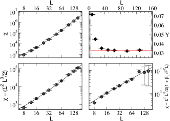
Figure 1: Plots of $\chi$ vs. $L$ (top left), $\chi-\Sigma^{2}L^{3}/2$ vs. $L$ (bottom left),$\chi-\Sigma^{2}L^{3}/2[1+\beta_{1}/(F^{2}L)]$ vs. $L$ (bottom right), and $Y$ vs. $L$ (top right) at $T=7.42$. The solid lines are fit to the data as discussed in the text.

In order to verify eq. (7), let us focus on $T=7.42$, a temperature which is below but close to $T_{c}$. We believe that the closeness to the second order transition point will reduce lattice artifacts and help make connections with ChPT easier. In the top-left graph of figure 1, we plot our results for $\chi$ as a function of $L$. The availability of results at large values of $L$ with small error bars allows us to fit our results to the first three terms in eq.(7) reliably. Using the values of $\chi$ for $L\geq 24$ we find $\Sigma=1.079(2)$, $F=0.181(4)$ and $a=114(4)$ with a $\chi^{2}/$d.o.f of $0.73$. In order to convince the readers that the error bars in our data are small enough to be sensitive to the higher order finite size effects, we also plot $\chi-\Sigma^{2}L^{3}/2$ versus $L$ in the bottom-left graph and $\chi-\Sigma^{2}L^{3}/2(1+\beta_{1}/(F^{2}L))$ versus $L$ in the bottom-right graph of figure 1. As the graphs indicate, the evidence for the $L^{2}$ and $L$ dependence of $\chi$ is indeed quite strong. Since $F^{2}=\lim_{L\rightarrow\infty}Y$, we can also compute $F$ independently using the helicity modulus. In the top right plot of figure 1 we plot $Y$ as a function of $L$. A fit indicates that the data for $L\geq 64$ is consistent with $F^{2}=0.0327(2)$ (solid line in the figure). This gives $F=0.181(1)$ in excellent agreement with the value obtained above. Thus, we find that the $L$ dependence of $\chi$ at $m=0$ and $T=7.42$ is indeed consistent with expectations from ChPT.

Let us now turn our attention to the entire region near $T_{c}$. Clearly, the fits based on ChPT (eq.(7)) will be reliable only for $L>>\xi$, where $\xi$ represents the diverging correlation length at $T_{c}$. In three dimensions $\xi\sim 1/F^{2}$. Since most of our computations involve lattice sizes with $L\leq 128$ we assume $1/F^{2}$ must be less than $64$ for our fits to be reliable. With this criterion we find that the above fitting procedure is reliable only when $T\leq 7.45$. The fits of our data in this range of temperatures are given in table 1.

$\beta$	$\Sigma$	$F$	$a$	$\chi^{2}$/d.o.f
7.30	1.599(5)	0.25(2)	6(12)	0.95
7.33	1.502(6)	0.26(2)	34(8)	1.5
7.40	1.198(11)	0.18(2)	62(11)	0.1
7.42	1.079(2)	0.181(4)	114(4)	0.73
7.43	1.014(3)	0.174(6)	142(6)	1.7
7.44	0.931(3)	0.149(7)	168(18)	0.15
7.45	0.827(9)	0.127(10)	242(25)	0.75

Table 1: Fits of $\chi$ vs. $L$ to eq. (7).

The values at $T=7.42$ have been discussed above. We can now verify if the values of $\Sigma$ given in table 1 satisfy eq. (8). However, we find that using $T_{c}$ as a free parameter in the fits is not ideal since the fits do not converge. Thus, we first determine $T_{c}$ using a different method.

Although, ChPT is unreliable on small lattices close to the phase transition, it can still help in roughly estimating $T_{c}$. We find that $7.476<T_{c}<7.478$. In this region we have data at four different temperatures: $7.4765,7.477,7.4775,7.478$. Since for these values of the temperature we expect $(T/T_{c}-1)L^{1/\nu}$ to be small, the $O(2)$ scaling suggests that in this temperature range $\chi$ must satisfy

$$\chi=g_{0}L^{1.962}+g_{1}(T/T_{c}\ -\ 1)L^{3.451},$$ (10)

obtained from eq. (9) after substituting the $O(2)$ critical exponents. Indeed, a joint fit to all the available data involving 22 data points yields $g_{0}=14.69(2)$, $g_{1}=-9.7(3)$ and $T_{c}=7.47739(3)$ with a $\chi^{2}/$d.o.f of $0.74$. This joint fit is shown in figure 2.

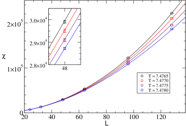
Figure 2: Plot of $\chi$ vs. $L$ for four different values of $T$ near $T_{c}$. The solid lines represent the function given in eq. (10) with $g_{0}=14.69$ and $g_{1}=-9.7$. The inset shows how the fitting function fits the data at $L=48$.

Interestingly, if we use the 3d Ising critical exponents in this fit instead of the $O(2)$ exponents, we obtain $T_{c}=7.47734(3)$ with a $\chi^{2}/$d.o.f of about $1$. Thus, clearly we cannot distinguish between Ising and $O(2)$ exponents with this approach. However, we believe we can determine $T_{c}$ quite accurately.

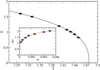
Figure 3: Plot of $\Sigma$ vs. $T$ at $m=0$ and $\langle\phi\rangle$ vs. $m$ at $T=T_{c}$ (Inset). The solid lines represent fits discussed in the text.

Having obtained $T_{c}$ we can now verify if the values of $\Sigma$ given in Table 1, for various values of $T$, satisfy eq. (8). In figure 3 we plot our results for $\Sigma$ as a function of $T$. We find that our data fits well to eq. (8) with $T_{c}=7.47739$ fixed. We obtain $A=2.92(2)$ and $\beta=0.348(2)$ with a $\chi^{2}/$d.o.f of $0.53$. Changing $T_{c}$ to $7.47734$ has negligible effect on this result. The value of $\beta$ is in excellent agreement with $0.3485(2)$, the exponent obtained in the three dimensional $XY$ spin model Cam01 and differs significantly with the three dimensional Ising exponent $0.32648(18)$ Cam99 .

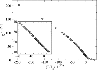
Figure 4: Plot of $\chi/L^{2-\eta}$ vs. $(T-T_{c})L^{1/\nu}$. The plot confirms the scaling prediction of eq.(9).

In order to test the scaling relation eq.(9) we plot $\chi/L^{2-\eta}$ against $(T-T_{c})L^{1/\nu}$ in figure 4. In order to be fair we do not include the data at $T=7.4765,7.477,7.4775$ and $7.478$, since these were already used to fit to this relation while determining $T_{c}$. The remaining data points (a total of 77) fall consistently on a single function as shown in figure 4.

So far we had focused on the physics at $m=0$. The algorithm discussed in Cha03 can easily be extended to include a quark mass. At $T=T_{c}$ one expects $\lim_{L\rightarrow\infty}\langle\phi\rangle=Bm^{1/\delta}$, where $\delta=4.780(2)$ in the case of $O(2)$ universality Cam01 . Since this is another independent test of the critical behavior and our prediction of $T_{c}$, in figure 3 (inset) we also show $\lim_{L\rightarrow\infty}\langle\phi\rangle$ as a function of $m$ at $T=T_{c}=7.47739$. The data fits well to the expected form with $B=5.9(1)$ and $\delta=4.97(10)$ with a $\chi^{2}/$d.o.f of $0.34$. On the other hand fixing $\delta=4.78$ in the fit gives $B=6.18(2)$ and increases the $\chi^{2}/$d.o.f to $0.88$.

V CONCLUSIONS

The above results show convincingly that the finite temperature chiral phase transition, in strongly coupled lattice QCD with staggered quarks, is governed by $O(2)$ universality class. Further, close to the transition in the low temperature phase the singularities of $O(2)$ ChPT arising due to Goldstone pions is observable.

There are many directions to extend the current work. In the low temperature phase one can verify the striking predictions of ChPT for the quark mass dependence of the chiral condensate, the pion mass and the pion decay constant. Using the pion decay constant as a physical scale it would also be interesting to understand the width of the critical region in physical units. This may shed some light on how difficult it would be to study the universal properties of the chiral transition at weaker couplings. The physics of the chiral limit of $SU(N)$ gauge theories at strong couplings in the presence of a baryon chemical potential is quite rich and has not yet been reliably explored from first principles. In particular when $N$ is even it is well known that the inclusion of a baryon chemical potential does not lead to sign problems. Although the phase diagrams of these models can be studied at weaker couplings (on small lattices away from the chiral limit) Kog03 , it would be interesting examine them at strong couplings (on large lattices in the chiral limit).

Current lattice QCD results at weaker couplings with light dynamical quarks suffer from large systematic errors. Bringing numerical precision, as demonstrated in this article, to these studies should be considered an important challenge to pursue in the future.

References

- (1) C. Bernard et. al., Nucl. Phys. B. (Proc. Suppl.) 119, 170 (2003).
- (2) J. Engels, S. Holtmann, T. Mendez and T. Schulze, Phys. Lett. B514 (2001) 299.
- (3) R. D. Pisarski and F. Wilczek, Phys. Rev. D29, 338 (1984).
- (4) F. Wilczek, Int. J. Mod. Phys. A7 3911 (1992).[Erratum-ibid. A7 (1992) 6951].
- (5) C. Bernard et. al., Phys. Rev. D61, 054503 (2000).
- (6) E. Laermann, Nucl. Phys. Proc. Suppl. 63, 114 (1998).
- (7) Y. Iwasaki et.al., Phys. Rev. Lett., 78, 17 (1997).
- (8) Y. Nishida, K. Fukushima, T. Hatsuda, arXiv:hep-ph/0306066.
- (9) N. Kawamoto and J. Smit, Nucl. Phys. B192, 100 (1981).
- (10) H. Kluberg-Stern, A. Morel and B. Petersson, Nucl. Phys. B215, 527 (1983).
- (11) P.H. Damgaard, N. Kawamoto and K. Shigemoto, Phys. Rev. Lett. 53, 2211 (1984).
- (12) P. Rossi and U. Wolff, Nucl. Phys. B248, 105 (1984).
- (13) G. Boyd et. al., Nucl. Phys. B376, 199 (1992).
- (14) H.G. Evertz, Adv.Phys. 52, 1 (2003).
- (15) S. Chandrasekharan and D.H. Adams, Nucl. Phys. B662, 220 (2003).
- (16) P. Hasenfratz and H. Leutwyler, Nucl. Phys. B343, 241 (1990).
- (17) M. Campostrini, M. Hasenbusch, A. Pelissetto, P. Rossi and E. Vicari, Phys. Rev. B63, 214503 (2001).
- (18) M. Campostrini, A. Pelissetto, P. Rossi and E. Vicari, Phys. Rev. E60, 3526 (1999).
- (19) J.B. Kogut, D.K. Sinclair and D. Toublan, arXiv:hep-lat/0305003.