A detailed study of the Abelian-projected SU(2) flux tube
and its dual Ginzburg-Landau analysis

Abstract

The color-electric flux tube of Abelian-projected (AP) SU(2) lattice gauge theory in the maximally Abelian gauge (MAG) is revisited. It is shown that the lattice Gribov copy effect in the MAG is crucial for the monopole-related parts of the flux-tube profiles. Taking into account both the gauge fixing procedure and the effect of finite quark-antiquark distance properly, the scaling property of the flux-tube profile is confirmed. The quantitative relation between the measured AP flux tube and the flux-tube solution of the U(1) dual Abelian Higgs (DAH) model is also discussed. The fitting of the AP flux tube in terms of the DAH flux tube indicates that the vacuum can be classified as weakly type-I dual superconductor.

I Introduction

An intuitive explanation why a quark cannot be isolated as a free particle rests on the assumption that the QCD vacuum has the property of a dual superconductor tHooft:1975pu ; Mandelstam:1974pi . Analogously to electrically-charged Cooper pairs being condensed in normal superconductors, magnetically-charged monopoles would be condensed in the QCD vacuum, and the dual analogue of the Meissner effect could be expected to occur. In the result, for example, the color-electric flux connecting a quark-antiquark ($q$-$\bar{q}$) system would be squeezed into a quasi-one-dimensional flux tube Abrikosov:1957sx ; Nielsen:1973ve ; Nambu:1974zg . This configuration provides a linearly rising potential between the quark and antiquark such that a quark cannot be separated infinitely from an antiquark spending a finite amount of energy.

Remarkably, lattice QCD simulations with ’t Hooft’s Abelian projection tHooft:1981ht , typically in the maximally Abelian gauge (MAG), support this picture numerically. The distributions of the electric field and of the magnetic monopole currents, which can be identified after Abelian projection, have been measured in the presence of a static $q$-$\bar{q}$ pair (represented by a Wilson loop) within pure SU(2) Singh:1993jj ; Matsubara:1994nq and SU(3) lattice gauge theories Matsubara:1994nq . It has been shown that the electric flux is confined in a dual Abrikosov vortex due to a monopole current circulating around the $q$-$\bar{q}$ axis, signalling the dual Meissner effect. More quantitatively, the London penetration length of the electric field has been studied systematically within SU(2) lattice gauge theory Cea:1995zt . These authors compared the penetration length in MAG with a gauge invariant definition of the flux-tube profile. They came to the conclusion that the penetration length is gauge independent. A large-scale simulation on a $32^{4}$ lattice at a single value of $\beta=2.5115$ within SU(2) lattice gauge theory has been performed next Bali:1998gz , applying the fine-tuned gauge fixing algorithm (a mixture of overrelaxation (OR) algorithm and a realization of simulated annealing (SA)) Bali:1996dm in order to fight the lattice Gribov copy problem in MAG and applying a noise reduction technique, the smearing of spacelike link variables before constructing a Wilson loop Bali:1996dm . Through this study, the dual Ampère law, a relation between the monopole current and the curl of electric field, has been confirmed with high accuracy.

What is interesting and suggestive is that these numerical results gave strong hints towards the existence of a dual Abelian Higgs (DAH) model (we often call this the dual Ginzburg-Landau (DGL) model) as an effective model to deal with the QCD vacuum Suzuki:1988yq ; Maedan:1988yi ; Suganuma:1995ps and with quark-induced hadronic excitations of the vacuum. In particular, the DAH model has a flux-tube solution corresponding to a $q$-$\bar{q}$ system. The mechanism of the flux-tube formation is nothing but the dual Meissner effect. The DAH model essentially contains three parameters, the dual gauge coupling $\beta_{g}$, the masses of the dual gauge boson $m_{B}$ and of the monopoles $m_{\chi}$. The inverses of these masses are identified as the London penetration length and the Higgs coherence length, respectively. These lengths determine the width of the flux tube. The so-called Ginzburg-Landau parameter is defined as the ratio between the two masses, $\kappa=m_{\chi}/m_{B}$, where the vacuum for $\kappa<1$ $(>1)$ is classified as type-I (type-II) superconductor.

Determining the parameters of the DAH model, based on the comparison between the most elementary flux-tube profile measured in non-Abelian lattice gauge theory and the flux-tube solution of the DAH model, is expected to be an important source of information on the QCD-vacuum structure itself, which would be helpful to learn about how the vacuum can function as a dual superconductor. Moreover, it might be useful in view of possible applications of the model in more complex physical situations (to describe baryons, for example in the SU(3) case). The first motivation has been, more or less, common to the above mentioned works and, in fact, such quantitative level of investigation has been attempted in Refs. Singh:1993jj ; Matsubara:1994nq ; Cea:1995zt ; Bali:1998gz . For example, the lattice data have been fitted by some approximate, analytical flux-tube solutions of the DAH model, and in this way the GL parameter have been estimated. The conclusions have varied, ranging from the vacuum belonging to the borderline between a type-I and type-II superconductor, with $\kappa\sim 1$, as claimed in Refs. Singh:1993jj ; Matsubara:1994nq , to a classification of the vacuum as a type-I superconductor, with $\kappa<1$, in Ref. Bali:1998gz . The reanalysis of the profile data in Ref. Bali:1998gz by fitting them with a numerical solution of the DAH model has supported the case of $\kappa\sim 1$ Gubarev:1999yp .

However, the systematic analysis of lattice flux-tube data in MAG itself was incomplete such that doubts have remained whether the resulting parameters represent physical reality. At least, one has to check several basic properties of the lattice flux-tube profile before one can seriously discuss the implications of the extracted DAH parameters. To mention the first, since one applies the MAG fixing, the lattice Gribov copy effect should be controlled, where the OR-SA algorithm would be helpful for this purpose Bali:1996dm . At second, one should check the scaling property of the profile with respect to changing the gauge coupling $\beta$ of the lattice simulation. At third, one has to inquire how the profile behaves as a function of the $q$-$\bar{q}$ distance. One also should know how to compare the lattice flux-tube profile with the flux-tube solution in the DAH model, if the above mentioned quantitative analysis is of interest.

In our previous paper Koma:2003gq , which was mainly devoted to the duality relating non-Abelian lattice theory on one hand with the DAH model on the other, we have carefully studied the flux-tube structure in the U(1) DAH model and have confronted it with some related data from our corresponding ongoing SU(2) lattice gauge measurements in the MAG. These studies, which will be discussed in the present paper in much more detail, have been done using a $32^{4}$ lattice with the OR-SA algorithm and with the smearing technique as in Ref. Bali:1996dm . Then, based on the Hodge decomposition of the Abelian Wilson loop into the electric photon and the magnetic monopole parts, we have found there that the Abelian-projected lattice flux tube consists of two components, the Coulombic and the solenoidal electric field, the latter being induced by the monopole currents circulating around the $q$-$\bar{q}$ axis. All this was in full analogy to the structure of the DAH flux-tube solution. We have also found Koma:2003gq that the Coulomb contribution cannot be neglected for any flux-tube length practically accessible in present-day lattice studies.

In this paper we are going to present all our results concerning the flux-tube profile within AP-SU(2) lattice gauge theory, obtained in the MAG, in a more complete way in order to meet the above requirements. The strategy of our study has been the following one. Measurements have been performed using a $32^{4}$ lattice at various $\beta$ values ($\beta$=2.3, 2.4, 2.5115, and 2.6). At first, we have investigated the lattice Gribov effect by comparing the profiles obtained from the widely used OR algorithm and from the OR-SA algorithm. In the context of the latter algorithm, we have also investigated the dependence on the number of gauge copies under investigation. At second, we have studied the scaling property of the flux-tube profile by comparing the profiles from various $\beta$ values, keeping the physical $q$-$\bar{q}$ distance approximately the same. The physical scales, the lattice spacing $a(\beta)$ for different values of $\beta$, have been calculated through the measurement of the corresponding non-Abelian string tension. Throughout the profile measurements, smearing has always applied to the spatial link variables before constructing a Wilson loop. This procedure is meant to extract the profiles which effectively belong to the ground state of a flux tube; we have checked the (in)dependence of the flux-tube profile on the temporal extension of the Wilson loop. This effect has not received the due attention in the previous studies in Refs. Singh:1993jj ; Matsubara:1994nq ; Cea:1995zt ; Bali:1998gz . This needs to be checked carefully when the Wilson loop is used to represent a static $q$-$\bar{q}$ source and the ground state is of interest. This procedure finally helps to reduce the noise. In a final step, we have assessed the DAH parameters by fitting the lattice data against the numerical DAH flux-tube solution. For this fit, we have not used the infinitely long flux-tube solution as it has been done in previous analyses Singh:1993jj ; Matsubara:1994nq ; Cea:1995zt ; Bali:1998gz ; Gubarev:1999yp . It should be noted that the use of the infinitely long solution would be suitable only for that part of the electric field which is induced by the monopole part of the Wilson loop with sufficiently large temporal length Koma:2003gq . For our purpose to assess the DAH parameters, in this way we have taken into full account the finite $q$-$\bar{q}$ length effect in the fit.

The paper is organized as follows. In section II we describe the procedures how to measure the Abelian-projected SU(2) flux-tube profile in MAG. Section III presents the numerical results. In section IV we describe the results of fitting the lattice profiles by the DAH flux-tube solutions. Section V is a summary and contains our conclusions. Preliminary results of the studies summarized in the present paper have been presented at the LATTICE2002 conference Koma:2002uq and in Ref. Koma:2003gq .

II Numerical procedures

In this section, we explain how to measure the profile of a color-electric flux tube on the lattice within the maximally Abelian gauge (MAG). We also develop the strategy to achieve a systematic, more detailed study of the flux-tube profile which takes into account the effect of the finite $q$-$\bar{q}$ length properly. We restrict the explanations of the methods to the case of SU(2) gauge theory.

The numerical study of the flux-tube profile begins with the simulation of non-Abelian gauge fields. A thermalized ensemble of SU(2) gauge configurations $\{U_{\mu}(m)\}$ is generated by simulating the standard Wilson action

$$S_{\rm SU(2)}[U]=\beta\sum_{m}\sum_{\mu<\nu}\left\{1-\frac{1}{2}{\rm Re}\;{\rm tr}[U_{\mu\nu}(m)]\right\}$$ (1)

using the Monte Carlo heatbath method. Here $U_{\mu\nu}(m)\in SU(2)$ are plaquette variables constructed in terms of link variables $U_{\mu}(m)\in SU(2)$ as

$$U_{\mu\nu}(m)\equiv U_{\mu}(m)U_{\nu}(m+\hat{\mu})U_{\mu}^{\dagger}(m+\hat{\nu})U_{\nu}^{\dagger}(m)\;.$$ (2)

The inverse coupling is given by $\beta=4/e^{2}$.

II.1 Maximally Abelian Gauge fixing

We put all the equilibrium configurations into the MAG. One exploits the gauge freedom of the SU(2) link variables with respect to gauge transformations $g(m)$

$$U_{\mu}(m)\mapsto U_{\mu}^{g}(m)=g(m)U_{\mu}(m)g^{\dagger}(m+\hat{\mu})$$ (3)

in order to achieve a maximum of the following gauge functional

$$R[U^{g}]=\frac{1}{8V}\sum_{m,\mu}{\rm tr}\left\{\tau_{3}U_{\mu}^{g}(m)\tau_{3}U^{g\;\dagger}_{\mu}(m)\right\}\;,$$ (4)

where $V$ is the number of sites in the lattice. The set of $g(m)\in SU(2)/U(1)$ for all site $m$ represents the MAG fixing gauge transformation defined on $m$.

For the numerical task to find the “optimal” $g(m)$, in the past mostly an overrelaxation (OR) algorithm has been used. However, as it has been pointed out in the work in Ref. Bali:1996dm , the OR algorithm is prone to fall into the nearest local maximum of Eq. (4) although the absolute maximum is of interest. This is due to the existence of many local maxima, which is known as the lattice Gribov copy problem. The only way known before to reduce the risk of being trapped in a wrong maximum is to explore many such local maxima by repeating the OR algorithm, starting each time from a new random gauge copy of the original Monte Carlo configuration; the ensemble of $U_{\mu}^{g}(m)$ corresponding to only the highest of the achieved maxima was then understood as the gauge-fixed ensemble. It has then been proposed to use a “simulated annealing (SA)” algorithm with a (final) OR algorithm in order to prevent very poor maxima from entering the competition between gauge copies Bali:1996dm . We may call this the OR-SA algorithm, which we mainly apply to fixing the MAG in the present paper. In the SA algorithm, the functional $R[U^{g}]$ is regarded as a spin action

$$F(S)=R[U^{g}]=\frac{1}{8V}\sum_{m,\mu}{\rm tr}\left\{S(m)U_{\mu}(m)S(m+\hat{\mu})U^{\dagger}_{\mu}(m)\right\},$$ (5)

where $S(m)=g^{\dagger}(m)\tau_{3}g(m)$ corresponds to spin variables. The maximization of this functional is achieved by considering the statistical system given by the partition function

$$Z=\sum_{\{S(m)\}}\exp\left[\frac{1}{\tau}F(S)\right]$$ (6)

with decreasing the auxiliary temperature $\tau\to 0$. Practically, we first prepare a thermalized spin system at a certain high temperature, which is decreased gradually according to some annealing schedule until sufficiently low temperature is reached ($\tau\approx 0$). Then, final maximization is done by means of the OR algorithms. Notice that this algorithm only succeeds to escape from the worst local maxima, such that the above-mentioned inspection of many gauge copies per Monte Carlo configuration cannot be avoided.

After the MAG fixing (3), the SU(2) link variables $U_{\mu}^{g}(m)=U_{\mu}^{\mathit{MA}}(m)$ are factorized into a diagonal (Abelian) link variable $u_{\mu}(m)\in U(1)$ and the off-diagonal (charged matter field) parts $c_{\mu}(m)$, $c_{\mu}^{*}(m)\in SU(2)/U(1)$ as follows

$$U_{\mu}^{\mathit{MA}}(m)=\left(\begin{array}[]{cc}\sqrt{1-|c_{\mu}(m)|^{2}}&-c_{\mu}^{*}(m)\\ c_{\mu}^{*}(m)&\sqrt{1-|c_{\mu}(m)|^{2}}\end{array}\right)\left(\begin{array}[]{cc}u_{\mu}(m)&0\\ 0&u_{\mu}^{*}(m)\end{array}\right)\;.$$ (11)

The Abelian link variables $u_{\mu}(m)$ are explicitly written as

$$u_{\mu}(m)=e^{i\theta_{\mu}(m)}\quad(\theta_{\mu}(m)\in[-\pi,\pi))\;.$$ (12)

The Abelian plaquette variables are constructed from the phase $\theta_{\mu}(m)$ as

$$\theta_{\mu\nu}(m) \equiv \theta_{\mu}(m)+\theta_{\nu}(m+\hat{\mu})-\theta_{\mu}(m+\hat{\nu})-\theta_{\nu}(m)\quad(\theta_{\mu\nu}(m)\in[-4\pi,4\pi))\;,$$ (13)

which can be decomposed into a regular part $\bar{\theta}_{\mu\nu}(m)\in[-\pi,\pi)$ and a singular (magnetic Dirac string) part $n_{\mu\nu}(m)=0,\pm 1,\pm 2$ as follows

$$\theta_{\mu\nu}(m) \equiv \bar{\theta}_{\mu\nu}(m)+2\pi n_{\mu\nu}(m)\;.$$ (14)

The field strength is defined by $\bar{\theta}_{\mu\nu}(m)=\theta_{\mu\nu}(m)-2\pi n_{\mu\nu}(m)$. Following DeGrand and Touissaint DeGrand:1980eq , magnetic monopoles are extracted from the magnetic Dirac string sheets as their boundaries

$$k_{\mu}(\tilde{m})=-\frac{1}{2}\varepsilon_{\mu\nu\rho\sigma}\partial_{\nu}n_{\rho\sigma}(m+\hat{\mu})\qquad(\varepsilon_{1234}=1)\;,$$ (15)

where $k_{\mu}(\tilde{m})=0,\pm 1,\pm 2$ and $\tilde{m}$ denotes the dual site defined by $\tilde{m}=m+(\hat{1}+\hat{2}+\hat{3}+\hat{4})/2$. Note that the monopole current satisfies a conservation law $\partial_{\mu}^{\prime}k_{\mu}(\tilde{m})=0$ formulated in terms of the backward derivative $\partial_{\mu}^{\prime}$.

II.2 Correlation functions of Wilson loops involving local probes

To find the flux-tube profile, one needs to measure the expectation value of a local probe ${\cal O}(m)$ with an external source as $\langle{\cal O}(m)\rangle_{j}$ (in our case $j$ corresponds to an Abelian Wilson loop). Based on the path integral representation of $\langle{\cal O}(m)\rangle_{j}$, it can be rewritten as the ratio of $\langle W_{A}{\cal O}(m)\rangle_{0}$ and $\langle W_{A}\rangle_{0}$, where the subscript $0$ means the expectation value in the vacuum without such a source Koma:2003gq :

$$\langle{\cal O}(m)\rangle_{j}=\frac{\langle W_{A}{\cal O}(m)\rangle_{0}}{\langle W_{A}\rangle_{0}}\;.$$ (16)

The Abelian Wilson loop is defined in terms of the $u_{\mu}(m)$

$$W_{A}(L)=\prod_{m\in L}u_{\mu}(m)=\exp[i\!\sum_{m\in L}\theta_{\mu}(m)]\;.$$ (17)

The local operators ${\cal O}(m)$ that we need to describe the structure of the flux tube are an electric field operator

$$i\bar{\theta}_{i4}(m)=i(\theta_{i4}(m)-2\pi n_{i4}(m)),$$ (18)

and a monopole current operator

$$2\pi ik_{i}(\tilde{m})\;,$$ (19)

where only spatial directions $i=1,2,3$ are of interest. To avoid the contamination from higher states as much as possible, we have inserted the local probe ${\cal O}(m)$ at $t=t_{m}=T/2$ to minimize the effect from the boundary of the Wilson loop at $t=0$ and $T$. The local field operators are then evaluated over the whole $x$-$y$ midplane erected in the center of the spatial extension of the Abelian Wilson loop ($z=z_{m}=R/2$). In other words, the coordinates of the local operator are $m=(x,y,z_{m},t_{m})$ running over the midplane of the flux tube between a quark and an antiquark.

II.3 Decomposition of the Abelian Wilson loop

In order to see the composed structure of the flux-tube profiles, it is useful to apply the Hodge decomposition to the Abelian Wilson loop, which allows us to define the photon and monopole Wilson loops. We have shown in the previous work Koma:2003gq for the electric field profile that the photon Wilson loop induces exclusively the Coulombic electric field while the monopole Wilson loop creates the solenoidal electric field. At the same time, concerning the monopole current profile, the photon Wilson loop is not correlated with the monopole currents, while exclusively the monopole Wilson loop is responsible for the monopole current signal.

We explain the decomposition using lattice differential form notations Chernodub:1997ay . The Abelian Wilson loop in Eq. (17) is written as $W_{A}=\exp[i(\theta,j)]$, where $\theta(C_{1})$ and $j(C_{1})$ are the Abelian link variables and the closed electric current. The Hodge decomposition of Abelian link variables leads to

$$\theta = \Delta^{-1}\Delta\theta=\Delta^{-1}(d\delta+\delta d)\theta$$ (20)

$$= \Delta^{-1}d\delta\theta+\Delta^{-1}\delta\bar{\theta}+2\pi\Delta^{-1}\delta n\;,$$

where the second and third terms are identified as the photon link ($\theta^{ph}=\Delta^{-1}\delta\bar{\theta}$) and monopole link ($\theta^{mo}=2\pi\Delta^{-1}\delta n$) variables, respectively. We do not need to fix the Abelian gauge in order to specify the first term in the second line, since it does not contribute to the Abelian Wilson loop due to $\delta j=0$: $(\Delta^{-1}d\delta\theta,j)=(d\Delta^{-1}\delta\theta,j)=(\Delta^{-1}\delta\theta,\delta j)=0$. Note that $\Delta$ is a lattice Laplacian and $\Delta^{-1}$ is its inverse, corresponding to the lattice Coulomb propagator. We have used $d\theta=\bar{\theta}+2\pi n$ (see, Eq. (14)) at the last equality. Inserting Eq. (20) into the expression of $W_{A}$, the Abelian Wilson loop is decomposed as

$$W_{A}[j]=\exp[i(\theta^{ph},j)]\cdot\exp[i(\theta^{mo},j)]\equiv W_{\mathit{Ph}}[j]\cdot W_{\mathit{Mo}}[j]\;.$$ (21)

We call $W_{\mathit{Ph}}$ and $W_{\mathit{Mo}}$ the photon Wilson loop and the monopole Wilson loop. They are separately used to evaluate the photon and monopole parts of the profiles.

II.4 Smearing of spatial links

The shape of the flux-tube profile induced by a Wilson loop depends on its size, $R\times T$, where $R$ corresponds to the $q$-$\bar{q}$ distance and $T$ the temporal extension. This means that the profile is influenced not only by the ground state but also by excited states, when a Wilson loop is used as an external source. If one is interested in the ground state, e.g., for the comparison with the flux-tube solution in the three-dimensional DAH model, in principle, one needs to know the profile at $T\to\infty$. However, it is practically impossible to take this limit due to the finite lattice volume.

Smearing is a useful technique to extract the profiles which belong to the ground state of a flux tube effectively even with a finite $T$. We then see remarkable noise reduction when the size of the Wilson loop is large. The procedure is as follows. Regarding the fourth direction as the Euclidean time direction, we perform the following step several ($N_{s}$) times for the spacelike Abelian link variables:

$$\exp[i\theta_{i}(m)]\mapsto\alpha\exp[i\theta_{i}(m)]+\sum_{j\neq i}\exp\left[i(\theta_{j}(m)+\theta_{i}(m+\hat{j})-\theta_{j}(m+\hat{i}))\right]\;,$$ (22)

where $i,j=1,2,3$ and $\alpha$ is an appropriate smearing weight.

To find an appropriate set of parameters ($\alpha$, $N_{s}$), one needs to investigate the $T$-dependence of several quantities like the ground state overlap and the $q$-$\bar{q}$ potential. The emerging shape of the profile also should be checked for the effect of smearing. A numerical example at $\beta=2.5115$ is shown in Appendix A. We notice that this procedure seems to have practical limitations which become visible in the flux-tube profile measurement. For the profile extracted with Wilson loops of size $R\leq T$, it works very well with large class of the parameter set ($\alpha$, $N_{s}$). We could easily observe $T$-independence of the profile within the numerical error. On the other hand, for the Wilson loops of size $R>T$, an extremely fine-tuned parameter set is required for smearing. However, we did not spend full effort to fix it.

III Numerical results

In this section, we present numerical results of the flux-tube profiles measured over the $x$-$y$ midplane of the $q$-$\bar{q}$ system (separated in $z$ direction) using the Abelian, photon and monopole Wilson loops. We are going to clarify i) the lattice Gribov copy effect associated with the MAG fixing procedure and ii) the scaling property.

The numerical simulations were done at $\beta=$ 2.3, 2.4, 2.5115, and $\beta=2.6$. The lattice volume was always $V=32^{4}$. We have used 100 configurations for measurements. We have stored them after 3000 thermalization sweeps, and they were separated by 500 Monte Carlo updates. To study (i), we have generated several numbers of gauge copies from a given SU(2) configuration by random gauge transformations, each of which has undergone the OR-SA algorithm in the process of MAG fixing. The SA algorithm itself is applied with the temperature decreasing from $\tau=2.5$ to $\tau=0.01$. After that the OR algorithm is adopted with a certain convergence criterion. As the number of gauge copies, we have chosen $N_{g}=$ 5, 10 and 20, and have stored the configurations which provide the best maximal value of the gauge functional Eq. (4) within these $N_{g}$. We have also stored the same number of configurations (=100) from the OR algorithm in the MAG fixing with the same stopping criterion as in the OR-SA case, where always the first copy has been accepted ($N_{g}=1$). To study (ii), we have used the configurations from the sample based on $N_{g}=$ 20 copies. The Abelian smearing parameters have been chosen $N_{s}=8$ for $\alpha=2.0$. With this choice, the temporal length independence of the profiles induced by the Abelian Wilson loop is achieved within errors, at least for $R\leq T$. The same procedure was also applied to the spacelike photon and monopole link variables before constructing each type of Wilson loop.

III.1 Fixing the physical scale and choosing the flux-tube lengths

The physical reference scale, the lattice spacing $a(\beta)$, has been determined from the non-Abelian string tensions $\sigma_{L}$ by fixing $\sqrt{\sigma_{phys}}=\sqrt{\sigma_{L}}/a\equiv 440$ MeV. The non-Abelian string tension has been evaluated by measuring expectation values of non-Abelian Wilson loops with optimized non-Abelian smearing. The emerging potential has been fitted to match the form $V(R)=C-A/R+\sigma_{L}\;R$. The resulting (dimensionless) lattice string tensions and the corresponding lattice spacings $a(\beta)$ in units of fm are shown in Table. 1.

Table 1: The non-Abelian string tensions and corresponding lattice spacings $a(\beta)$ for $\beta=$ 2.3, 2.4, 2.5115, and 2.6 estimated by the relation $a(\beta)=\sqrt{\sigma_{L}/\sigma_{phys}}$ with $\sqrt{\sigma_{phys}}=440$ MeV.

$\beta$	$\sigma_{L}$	$a(\beta)$ [fm]
2.3	0.144(3)1	0.170(2)
2.4	0.0712(5)	0.1197(4)
2.5115	0.0323(4)	0.0806(5)
2.6	0.0186(2)	0.0612(5)

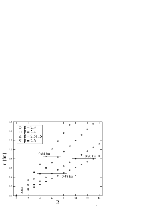
Figure 1: Estimate of the physical $q$-$\bar{q}$ distance $r$ in units of fm as a function of lattice distance $R$ for various $\beta=$ 2.3, 2.4, 2.5115, and 2.6 used in this study.

To compare the profiles from various $\beta$ values, it is quite important to put data into groups close to almost the same physical $q$-$\bar{q}$ distance because the finite length effect of the flux-tube system has to be studied simultaneously Koma:2003gq . One might naively expect that the flux-tube profile has a good translational-invariant property along the $q$-$\bar{q}$ axis so that the difference in length does not matter when one follows the change in lattice scale. However, as shown in our previous work Koma:2003gq , the finite length effect is not negligible as long as the photon part of the profile still contributes to the total profile. In Fig. 1 we then plot, for the four $\beta$-values at our disposal, the physical length $r=Ra(\beta)$ in units of fm for various choices of the integer lattice flux-tube length $R$. This information is taken into account when we study the scaling property of the flux-tube profile.

III.2 Assessment of the lattice Gribov problem

We investigate how the flux-tube profile depends on the lattice Gribov copy effect due to the MAG fixing. As shown in Ref. Bali:1996dm , the density of monopole currents (in vacuum) is sensitive to the gauge fixing procedure; it decreases when larger $R[U^{g}]$ is achieved. Therefore, we expect that the monopole-related part of the profile crucially depends on the quality of the gauge fixing procedure.

In Fig. 2 we show the electric field and monopole current profiles as observed over the flux-tube midplane at $\beta=2.3$ for $W(R,T)=W(3,3)$. Profiles, both with the use of the OR and the OR-SA algorithms, are presented. The dependence on the number of gauge copies under exploration is also investigated for the case of the latter algorithm. The upper, middle, and lower figures are the profiles from the Abelian, the monopole and the photon Wilson loops, respectively.

We observe that the electric field and the monopole current profiles (except from the photon Wilson loop) are overestimated if the OR algorithm is applied. A possible explanation of this behavior is the following. The correlation between the monopole Wilson loop and the monopole currents are enhanced artificially due to denser monopole current system owing to the imperfect gauge fixing, which results in a larger contribution to the monopole current profile. Then, the strongly circulating monopole current around the $q$-$\bar{q}$ axis induces a strong solenoidal electric field. In this way, the electric field profile is also overestimated when the OR algorithm is adopted. It is interesting to note that since the photon Wilson loop is not correlated with the monopole currents, the corresponding electric field profile is insensitive to the Gribov copy problem. Finally, the impact of the Gribov copy problem on the monopole part is inherited also by the total flux-tube profile measured by the Abelian Wilson loop. Notice that the number of gauge copies to which the OR-SA algorithm is applied does not drastically change the profiles compared with the change from OR to OR-SA algorithm. This suggests that the tentative maxima successfully anticipated at the end of SA algorithm do not strongly differ in the monopole density.

In Figs. 3, 4 and 5 we show the same plot as in Fig. 2 for other $\beta$ values, correspondingly choosing the Wilson loops: at $\beta=2.4$ for $W(4,4)$, at $\beta=2.5115$ for $W(6,6)$ and at $\beta=2.6$ for $W(8,8)$. Here, the physical sizes of the respective Wilson loops are approximately the same (0.48 fm $\times$ 0.48 fm). We find that with increasing $\beta$ (approaching to the continuum limit), the difference between the profiles from the OR algorithm and the OR-SA algorithm becomes clearer, i.e. the effect of the Gribov copy problem becomes more significant. Since the continuum limit is of interest, one needs to take care of this problem as already emphasized in Ref. Bornyakov:2001ux .

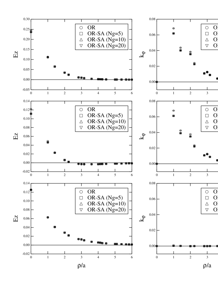
Figure 2: The profiles of electric field (left) and monopole current (right) at $\beta=2.3$ for the $W(3,3)$ quark-antiquark system for gauge fixing according to OR and OR-SA algorithms, respectively, and the dependence on the number of gauge copies in the OR-SA case. Non-integer radiuses appear due to off-axis distances from the flux-tube axis. Upper, middle, and lower figures refer to correlations with the full Abelian, the monopole and the photon Wilson loops.

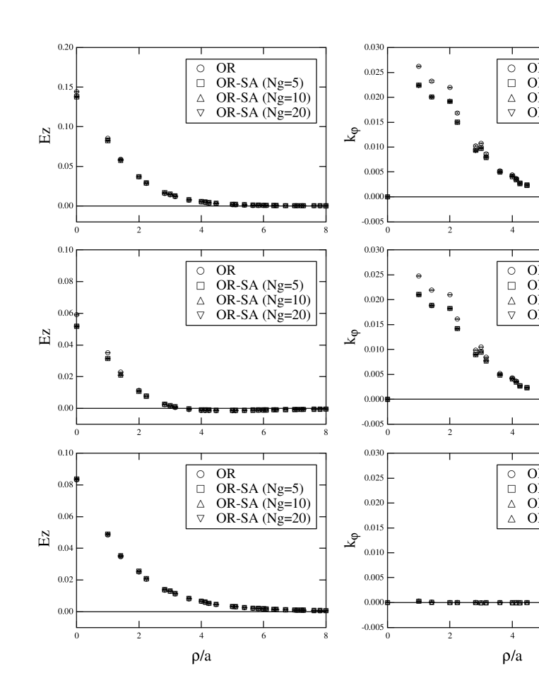
Figure 3: The same plot as in Fig. 2 at $\beta=2.4$ for $W(4,4)$.

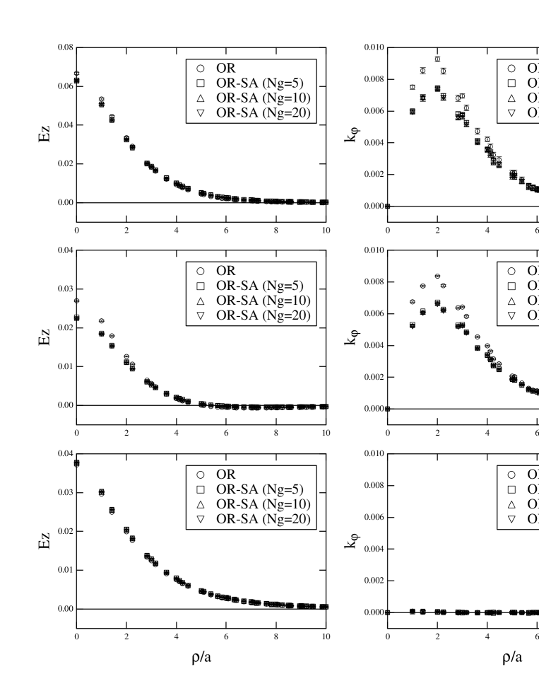
Figure 4: The same plot as in Fig. 2 at $\beta=2.5115$ for $W(6,6)$.

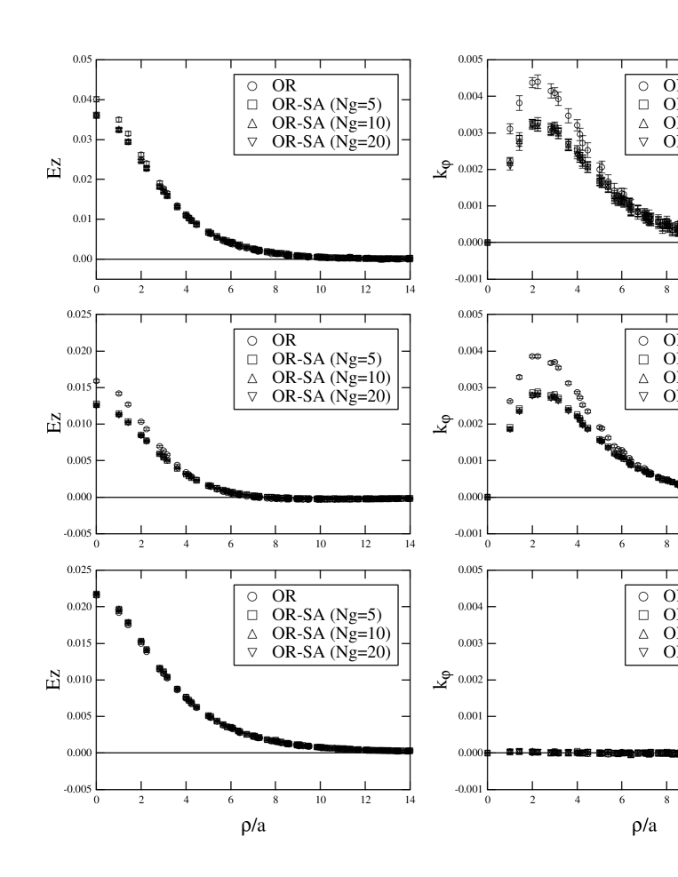
Figure 5: The same plot as in Fig. 2 at $\beta=2.6$ for $W(8,8)$.

III.3 Does the flux-tube profile satisfy scaling ?

We investigate the scaling property for groups of $q$-$\bar{q}$ distances according to Fig. 1 using the best MAG-fixed configurations with $N_{g}=20$. We choose three sets of physical distances:

• at $r\sim 0.48$ fm: from $\beta=$2.4 with $W(R,T)=W(4,4)$, $\beta=$2.5115 with $W(6,6)$, and $\beta=$2.6 with $W(8,8)$,

• at $r\sim 0.80$ fm: from $\beta=$2.5115 with $W(10,6)$ and $\beta=$2.6 with $W(13,8)$.

• at $r\sim 0.84$ fm: from $\beta=$2.3 with $W(5,3)$ and $\beta=$2.4 with $W(7,4)$.

Here, the physical size of the temporal extension of the Wilson loop is taken approximately the same among all sets. This choice is made to normalize the systematic uncertainty for the flux-tube profile which might come from finite $T$ even after smearing, especially for Wilson loops having $R>T$, which reflect contributions from excited states. We did not attempt to include profiles from such Wilson loops into the fit in Sec. IV. The first set is shown in Fig. 6. The other two sets are plotted together in Fig. 7.

We find that both the electric and monopole current profiles measured at different $\beta$ values from the interval 2.3 to 2.6 scale properly for each of the three groups of $q$-$\bar{q}$ distances. The remaining minor differences can be blamed to small differences in $q$-$\bar{q}$ distance and uncontrolled smearing effects. We also observe the following properties. Although the rotational invariance around $q$-$\bar{q}$ axis is poor for small $\beta$, it is recovered with increasing $\beta$. The electric field profile from the photon Wilson loop is very sensitive to the change of the $q$-$\bar{q}$ distance. Clearly, the shape of the electric field profiles from the photon Wilson loop in Figs. 6 and 7 are different; this part of the electric field drastically decreases with increasing $q$-$\bar{q}$ distance. On the other hand, the electric field profile from the monopole Wilson loop remains almost the same with increasing $q$-$\bar{q}$ distance. The difference of the electric field profile coming from the full Abelian Wilson loop for different $q$-$\bar{q}$ distance can be explained by the change of the photon contribution. The large error of the monopole current profile from the Abelian Wilson loop in Fig. 7 is due to the large size of the Wilson loop, $13\times 8$, at $\beta=$ 2.6. The statistics is not sufficient in this case. However, it is interesting to find that the decomposition of the Abelian Wilson loop into the photon and monopole parts helps to see a clear signal even with a number of configurations which is normally used for smaller Wilson loops.

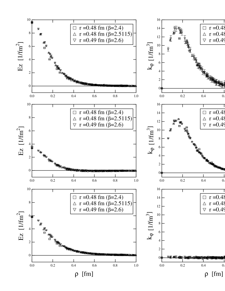
Figure 6: The $\beta$ dependence of the profiles of the electric field (left) and the monopole current (right) for $q$-$\bar{q}$ distance $r\sim$ 0.48 fm as a function of the flux-tube radius $\rho$ given in units of fm (see Table 1 and Fig. 1).

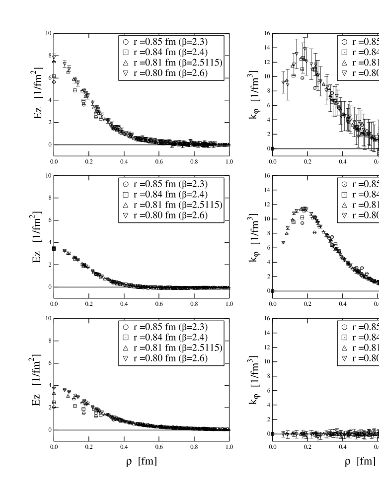
Figure 7: The same plot as in Fig. 6 for $q$-$\bar{q}$ distance $r\sim$ 0.80 and 0.84 fm (see Table 1 and Fig. 1).

IV Fitting with the U(1) DAH flux tube

In this section, we discuss the quantitative relation between the extracted AP-SU(2) flux tube and the classical flux tube of the dual Abelian Higgs model (the DAH flux tube) through a $\chi^{2}$ fit of the former profile by the latter. In the fit, we take into account both the electric field and the monopole current profiles simultaneously.

IV.1 The dual lattice formulation of the DAH model

The DAH flux-tube profile is calculated within the dual lattice formulation of the three dimensional DAH model in order to mimic eventual lattice discretization effects in the fit Koma:2000hw . The lattice DAH action is

$$S_{\rm DAH}=\beta_{g}\sum_{m}\left[\frac{1}{2}\sum_{i<j}F_{ij}(m)^{2}+\frac{m_{B}^{2}}{2}\sum_{i=1}^{3}\left|\Phi(m)-e^{iB_{i}(m)}\Phi(m+\hat{i})\right|^{2}+\frac{m_{B}^{2}m_{\chi}^{2}}{8}\left(|\Phi(m)|^{2}-1\right)^{2}\right],$$ (23)

where $F_{ij}$ is the dual field strength

$$F_{ij}(m)=B_{i}(m)+B_{j}(m+\hat{i})-B_{i}(m+\hat{j})-B_{j}(m)-2\pi\Sigma_{ij}(m)\,.$$ (24)

$B_{i}(m)$ and $\Phi(m)$ are the dual gauge field and the complex-valued scalar monopole field. The electric Dirac string $\Sigma_{ij}$ in the dual field strength reflects the actual length of the flux tube. For instance, for a straight flux tube along the $z$ direction, $\Sigma_{12}=1$ for all plaquettes penetrated by this flux tube, otherwise $\Sigma_{ij}=0$ Koma:2000hw . This action contains three parameters: the dual gauge coupling $\beta_{g}=1/g^{2}$, the dual gauge boson mass $m_{B}=\sqrt{2}gv$, and the monopole mass $m_{\chi}=2\sqrt{\lambda}v$. Here $v$ corresponds to the monopole condensate, and $\lambda$ is the self-coupling of the monopole field. Writing the masses in terms of $g$, $v$ and $\lambda$ is more familiar in the continuum form of the DAH model. Note that in the lattice formulation, all fields and parameters are dimensionless. The type of dual superconductivity is characterized by the Ginzburg-Landau parameter, $\kappa=m_{\chi}/m_{B}$. In this definition, the cases $\kappa<1$ $(>1)$ are classified as type I (type II) vacuum.

The flux-tube solution is obtained by solving the field equations. The equation for $B_{i}(m)$ is given by $\frac{\partial S_{\rm DAH}}{\partial B_{i}(m)}=\beta_{g}X_{i}(m)=0$. Similarly, the equations for the monopole field are $\frac{\partial S_{\rm DAH}}{\partial\Phi^{R}(m)}=\beta_{g}m_{B}^{2}X^{R}(m)=0$ and $\frac{\partial S_{\rm DAH}}{\partial\Phi^{I}(m)}=\beta_{g}m_{B}^{2}X^{I}(m)=0$. The superscripts $R$ and $I$ refer to the real and imaginary parts of the complex scalar monopole field. The explicit form of the field equations $X_{i}(m)$, $X^{R}(m)$, and $X^{I}(m)$ are given in Appendix B. To solve the field equations numerically, we adopt a relaxation algorithm a la Newton and Raphson by taking into account the second derivative of the action with respect to each field Koma:2000hw . We iterate this procedure until the conditions $\sum_{m}\sum_{i=1}^{3}(X_{i}(m))^{2}<0.0001$ and $\sum_{m}\{(X^{R}(m))^{2}+(X^{I}(m))^{2}\}<0.0001$ are satisfied and the change of the action for one iteration step $\Delta S_{\rm DAH}<0.001$. Within the possible range of the DAH parameters, we find that the solution is well-converged.

The strategy of the fit is as follows. We fit the flux-tube profile induced by the Abelian Wilson loop with the DAH flux tube. Since we want to use the $T$-independent profile and it can only be $T$-independent if $R\leq T$, we are restricted for this purpose (profile) to $R\leq T$. The electric field and monopole current profiles of the DAH flux tube is $\sqrt{\beta_{g}}\varepsilon_{ijk}F_{jk}$ and $\sqrt{\beta_{g}}K_{i}$ (see, Appendix B), which are regarded as representing $\bar{\theta}_{i4}$ and $2\pi k_{i}$ of the AP-SU(2) field profile (see, Eqs. (18) and  (19)). The DAH field profiles are calculated with the same spatial volume as used in the SU(2) simulation, namely $32^{3}$, imposing the same periodic boundary conditions for all three directions. The length of the DAH flux tube is taken equal to that of the AP-SU(2) flux tube to be fitted. We extract the profile all over the midplane cutting the flux tube between the quark and the antiquark. The DAH lattice spacing is assumed to be the same as $a(\beta)$ of the SU(2) lattice. Once the fit has found the optimal set of dimensionless DAH parameters, the physical masses are fixed with the help of $a(\beta)$. To seek the set of parameters which provides minimum $\chi^{2}$, we use the MINUIT code from the CERNLIB.

After getting the set of the DAH parameter, we check whether this set can reproduce the composed internal structure of the electric field profile as a superposition of the Coulombic plus the solenoidal field by applying the Hodge decomposition as in Eq. (20) to the dual field strength. Each field strength can be constructed from the DAH photon link ($B^{ph}=2\pi\Delta^{-1}\delta\Sigma$) and the DAH monopole link ($B^{mo}=\Delta^{-1}\delta F$), respectively. Note that the field strength from the photon (monopole) links describe the Coulombic (solenoidal) electric field.

IV.2 Fitting results

We fit the flux-tube profiles at $\beta=2.5115$ from $W(3,6)$, $W(4,6)$, $W(5,6)$, and $W(6,6)$, and at $\beta=2.6$ from $W(4,8)$, $W(5,8)$, $W(6,8)$, $W(7,8)$, and $W(8,8)$. Here, the physical length of the temporal extension of the Wilson loop for these $\beta$ values is approximately the same, $0.48$ fm. We did not attempt to fit the profiles from the Wilson loops with $R>T$, since they still contain the contribution from excited states ($T$ dependence) even after the smearing (see, Sec. II.4 and Appendix A). In the fit, we have taken into account the data from $\rho/a\geq 2$ for $\beta=2.5115$ and from $\rho/a\geq 3$ for $\beta=2.6$ to certain maximum radii which provide the positive expectation values for the field profiles. We have checked that the DAH parameters emerging from the fit are rather insensitive with respect to restricting the fit range (further increasing the minimal radius).

In Table 2, we summarize the parameters obtained by the fit. In Fig. 8, we show how the AP flux tube is described by the DAH one using the profiles from $W(6,6)$ at $\beta=2.5115$ and from $W(8,8)$ at $\beta=2.6$. One can see that the profiles from the Abelian Wilson loop are reproduced. Remarkably, the resulting DAH parameters also reproduce the composed internal structure of the AP flux tube as well. In this sense, the fit which takes into account the finite $q$-$\bar{q}$ distance works very well. In Fig. 9, we plot the fitting parameters as a function of the physical $q$-$\bar{q}$ distance, where the scale of the masses is recovered by using the SU(2) lattice spacing $a(\beta)$. The maximum physical $q$-$\bar{q}$ distance is around 0.5 fm. We find that the $\beta_{g}$ becomes large as increasing the $q$-$\bar{q}$ distance, $r=Ra(\beta)$, while the masses of the dual gauge boson and of the monopole are rather stable. The constant fit of the masses using the stable data for $r>0.3$ fm provides

$$m_{B}=1091(7)\;\mbox{MeV},$$ (25)

$$m_{\chi}=953(20)\;\mbox{MeV}.$$ (26)

The GL parameter is then found to be

$$\kappa=\frac{m_{\chi}}{m_{B}}=0.87(2)<1,$$ (27)

which means that the vacuum corresponds to weakly type I in terms of the classification of the dual superconductivity. However, we have noticed that the change of the dual gauge coupling $\beta_{g}$ as a function of $r$ indicates that the vacuum cannot completely be regarded as the classical one. In fact, if one defines an effective Abelian electric charge based on the Dirac quantization condition as $e_{\rm eff}=4\pi/g=4\pi\sqrt{\beta_{g}}$, this coupling shows an anti-screening behavior; $e_{\rm eff}$ becomes large with increasing $r$. The constant behaviors of $m_{B}$ and $m_{\chi}$ indicate that various widths of the AP flux tube, which are defined by the inverse of these masses (the penetration depth $m_{B}^{-1}$ and the coherence length $m_{\chi}^{-1})$, do not depend on $r$. This is established at least up to a $q$-$\bar{q}$ distance $r=0.5$ fm.

Table 2: The $q$-$\bar{q}$ distance dependence of the DAH parameter

$\beta$	$R$	$\beta_{g}$	$m_{B}$	$m_{\chi}$	$\chi^{2}$/dof	fit range
2.5115	3	0.0630(5)	0.4633(23)	0.3490(43)	135/67	$\rho/a\geq 2$
2.5115	4	0.0711(5)	0.4595(17)	0.3738(7)	99.9/81	$\rho/a\geq 2$
2.5115	5	0.0797(8)	0.4485(29)	0.4090(6)	77.4/81	$\rho/a\geq 2$
2.5115	6	0.0840(8)	0.4504(21)	0.4091(3)	186/97	$\rho/a\geq 2$
2.6	4	0.0719(9)	0.3372(72)	0.2284(371)	35.7/91	$\rho/a\geq 3$
2.6	5	0.0798(13)	0.3295(36)	0.2884(29)	22.0/91	$\rho/a\geq 3$
2.6	6	0.0834(12)	0.3368(31)	0.2673(11)	33.3/75	$\rho/a\geq 3$
2.6	7	0.0867(18)	0.3354(46)	0.3004(5)	37.3/91	$\rho/a\geq 3$
2.6	8	0.0907(14)	0.3360(10)	0.3081(2)	75.5/105	$\rho/a\geq 3$

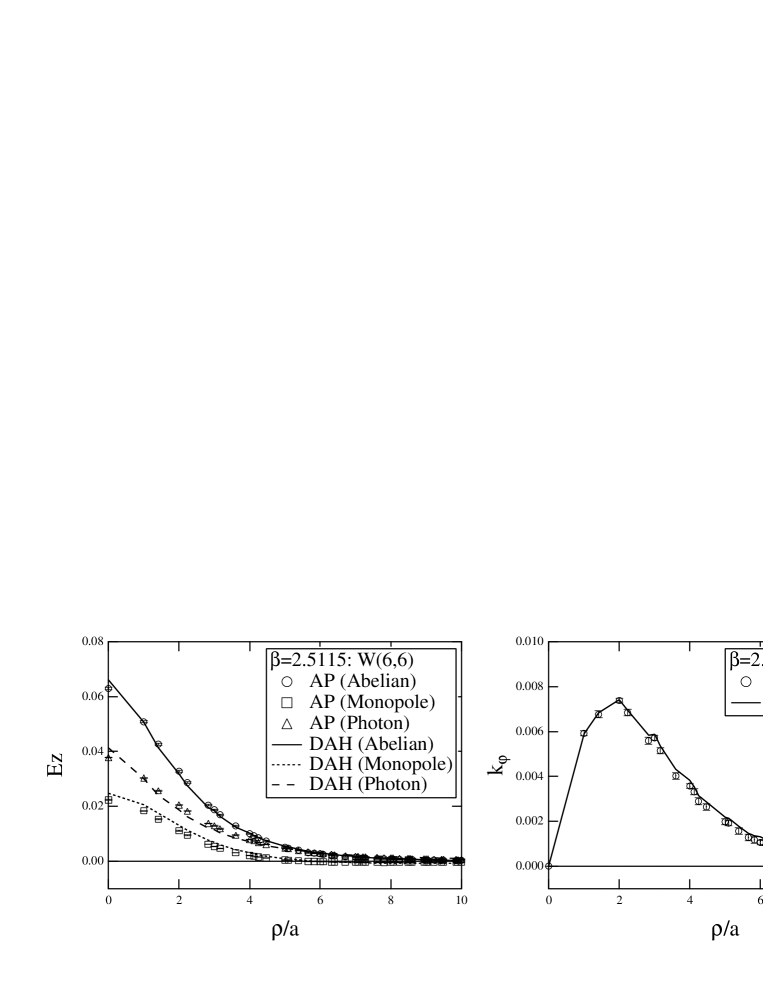
Figure 8: Some examples of the fitting at $\beta=2.5115$ for $R=6$ (upper row), and $\beta=2.6$ for $R=8$ (lower row). The solid line is the DAH flux-tube profile (obtained by the fit). The dotted and dashed lines correspond to its monopole and photon parts (as predicted using the fit parameters).

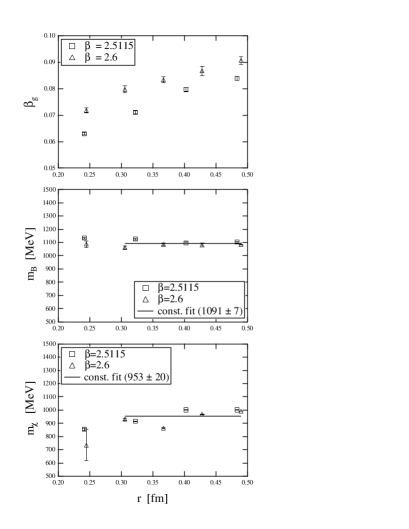
Figure 9: The DAH parameters $\beta_{g}$, $m_{B}$ and $m_{\chi}$ as functions of the physical $q$-$\bar{q}$ distance.

V Summary and conclusions

The main aim of this paper has been to present the flux-tube profile data within Abelian-projected (AP) SU(2) lattice gauge theory in the maximally Abelian gauge (MAG) in a quality and sufficiently detailed in order to warrant quantitative discussions from the point of view of the dual Abelian Higgs (DAH) model. We have mainly studied i) the lattice Gribov copy effect associated with the MAG fixing procedure and ii) the scaling property ($\beta$ independence) of the flux-tube profile using a large lattice volume, $32^{4}$. During these investigations, we have always paid special attention to the composed internal structure of the AP flux tube. We have also carefully monitored the effect of smearing.

(i) We have found that the flux-tube profile is very sensitive to lattice Gribov copy problem in the MAG, in particular, the monopole-related parts of the profile are strongly affected. The monopole current profile is overestimated if one uses a non-improved gauge fixing algorithm or just one single gauge copy. Since we do not know the real global maximum of $R[U^{g}]$ (see, Eq. (4)), we cannot insist that our result is the final one. However, we have obtained significantly corrected profile data by virtue of the over-relaxed simulated annealing algorithm converging within a moderate number of gauge copies.

(ii) We have confirmed the scaling property of the flux-tube profile, which has been achieved by using the well-gauge-fixed configurations and by taking into account the finite $q$-$\bar{q}$ distance effect properly. In fact, the flux-tube profile is strongly depending on the size ($R$ and $T$) of the Abelian Wilson loops $W(R,T)$. At finite $q$-$\bar{q}$ distance $R$, the photon part of the flux-tube profile is crucially contributing to the total Abelian electric field measured at any distance from the external charges.

Finally, we have investigated the effective parameters of the U(1) dual Abelian Higgs (DAH) model by fitting the AP flux tube with the DAH flux-tube solution. We have adopted a new fitting strategy; in order to obtain the DAH flux-tube solution, we have defined the DAH model on the dual lattice and have solved the field equations numerically with the same size of the spatial lattice volume ($32^{3}$) and with the same periodic boundary condition as in the AP-SU(2) simulations. In particular, we have fully taken into account the finite $q$-$\bar{q}$ distance effect. As a result, we also could reproduce the composed internal structure of the AP flux tube in terms of the DAH one. We have found that the dual gauge coupling depends on the $q$-$\bar{q}$ distance, which becomes large with increasing $q$-$\bar{q}$ distance. In this sense, the comparison between the AP flux tube and the DAH flux tube considered at the classical level is not perfect. On the other hand, we have found that the masses of the dual gauge boson and the monopole are almost constant as a function of the $q$-$\bar{q}$ distance up to 0.5 fm, which take values of 1100 MeV and 950 MeV, respectively. The Ginzburg-Landau parameter takes a value slightly smaller than unity, indicating that the vacuum is classified as weakly type-I dual superconductor.

We should mention that, while we have chosen the DeGrand-Toussaint prescription for the electric flux and the monopole currents featuring in the description of flux tube in the Abelian projected gauge theory, this choice is not unique. We have made our choice because of the possibility to relate then the AP theory to the DGL description Koma:2003gq . Haymaker et al. Cheluvaraja:2002yj , on the other hand, have proposed an alternative definition to satisfy the the Maxwell equations even at finite lattice spacing. It would also be interesting to study the differences of the measured flux-tube profile with their definition.

Suggested by an effective bosonic string description Luscher:1981iy , it is expected that the width of the flux tube broadens with increasing $q$-$\bar{q}$ distance. If such an effect exists in the effective DAH description, too, we would have to see the change of the DAH mass parameters as a function of the $q$-$\bar{q}$ distance. Our results show that, at least until 0.5 fm, the width of the flux tube is appearing as an almost stable vacuum property. It could be argued that the bosonic-string-like features of the flux tube might become manifest only for much more elongated strings. In order to study the existence of string roughening, one might be forced to study the profiles correlated with Wilson loops of much larger size. For larger $R$, if one takes small $T$, one can get the signal of the flux-tube profile with the help of smearing techniques. However, one has to care that such a profile does not immediately correspond to the physical profile at $T\to\infty$. In order to check if the flux tube becomes broader, the profile should be investigated in a $T$-independent regime.

It would be worthwhile to extend the strategy of this paper to the AP-SU(3) flux tube in order to discuss the quantitative relation between SU(3) gluodynamics and the U(1)$\times$U(1) DAH model.

Acknowledgment

We are grateful to M.I. Polikarpov for valuable discussions and the collaboration leading to our previous paper Koma:2003gq . We wish to thank V. Bornyakov, H. Ichie, G. Bali, P.A. Marchetti, V. Zakharov, R.W. Haymaker and T. Matsuki for their constructive discussions. We acknowledge also the collaboration of T. Hirasawa in an early stage of the present study. Y. K. and M. K. are grateful to P. Weisz for the discussion on the string fluctuation. M.K. is partially supported by Alexander von Humboldt foundation, Germany. E.-M. I. acknowledges gratefully the support by Monbu-Kagaku-sho which allowed him to work at Research Center for Nuclear Physics (RCNP), Osaka University, where this work has begun. He expresses his personal thanks to H. Toki for the hospitality. E.-M. I. is presently supported by DFG through the DFG-Forschergruppe ’Lattice Hadron Phenomenology’ (FOR 465). T. S. is partially supported by JSPS Grant-in-Aid for Scientific Research on Priority Areas No.13135210 and (B) No.15340073. The calculations were done on the Vector-Parallel Supercomputer NEC SX-5 at the RCNP, Osaka University, Japan.

Appendix A Fixing the smearing parameters

The smearing procedure for the spatial link variables as indicated in Eq. (22) successfully reduces the contribution from excited states. To find a set of optimized smearing parameters, the weight $\alpha$ and the number of smearing sweeps $N_{s}$, we need to investigate the behavior of the ratio

$$C_{0}\equiv[W_{A}(R,T)]^{T+1}/[W_{A}(R,T+1)]^{T}$$ (28)

as a function of $R$ for some fixed values of $T$ Bali:1996dm . For interpretation, we notice that this ratio turns into the ground state overlap in the limit $T\to\infty$. We apply the smearing step repeatedly on the spatial links until we get a good ground state overlap. In Fig. 10 we show the typical behavior of the ground state overlap before and after smearing at $\beta=2.5115$. We see clearly that $C_{0}$ got enhanced to $C_{0}\approx 1$ as the result of smearing. This justifies to select, for this $\beta$, the smearing parameters $\alpha=2.0$ and $N_{s}=8$ which have led to the improved ground state overlap. Using this set, we can also confirm a typical improvement of the Abelian potential

$$V(R,T)=\ln(W_{A}(R,T)/W_{A}(R,T+1))\;.$$ (29)

This is shown in Fig. 11, where the potential is plotted as a function of $T$ for some fixed $R$. After smearing, we see a clear pattern of plateaus ranging from $T=1$ to large $T$, the height of which corresponds to the values of the potential $V(R)$ at $T\to\infty$.

In Fig. 12, we show the effect of the smearing to the behavior of the flux-tube profile at $\beta=2.5115$ for $W(6,4)$, $W(6,6)$, and $W(6,8)$. Before smearing, the shape of the electric field and monopole current profiles are depending on the size of the Wilson loop; the profile from the smaller Wilson loop is enhanced. After the smearing, we see a reduction of the electric field for all cases and at least, the profiles from $W(6,6)$, and $W(6,8)$ coincide within the numerical error (the error is also reduced). This suggests that $T$-independence of the flux-tube profile is now achieved. The shape of the monopole current profile is insensitive to smearing. However, we find a remarkable reduction of the error. Note that the profile from $W(6,4)$ still did not converge into the same profile, which means that the chosen smearing parameter set is not adequate in this case.

Figure 10: The ground state overlap before (left) and after (right) smearing at $\beta=2.5115$.

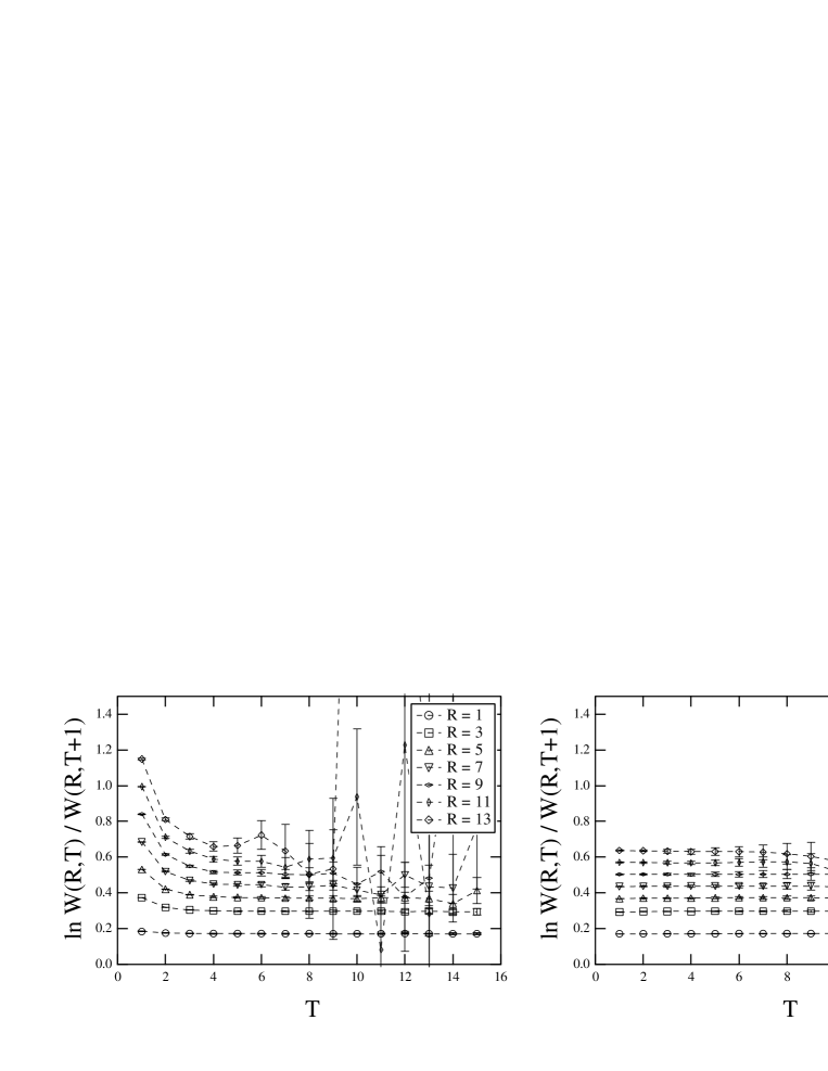
Figure 11: The potential before (left) and after (right) smearing at $\beta=2.5115$.

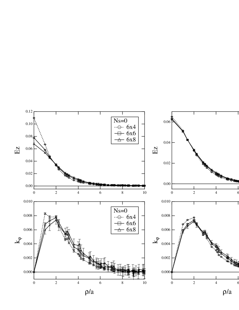
Figure 12: The flux-tube profiles before (left) and after (right) Abelian smearing at $\beta=2.5115$ for $R=6$ (fixed). Three cases of the temporal length, $T=4$, 6 and 8, are shown.

Appendix B Field equations of the lattice DAH model

We note the field equations of the lattice DAH model. For the dual gauge field,

$$\frac{\partial S}{\partial B_{i}(m)}=\beta_{g}X_{i}(m)=0,$$ (30)

where

$$X_{i}(m) = F_{ij}(m)+F_{ji}(m-\hat{j})+F_{ik}(m)+F_{ki}(m-\hat{k})-K_{i}(m)\;.$$ (31)

The last term corresponds to the monopole current

$$K_{i}(m) = -m_{B}^{2}\biggl{[}\Phi^{R}(m)\left(\Phi^{R}(m+\hat{i})\sin B_{i}(m)+\Phi^{I}(m+\hat{i})\cos B_{i}(m)\right)$$ (32)

$$-\Phi^{I}(m)\left(\Phi^{R}(m+\hat{i})\cos B_{i}(m)-\Phi^{I}(m+\hat{i})\sin B_{i}(m)\right)\biggr{]}\;.$$

For the monopole fields,

$$\frac{\partial S}{\partial\Phi^{R}(m)}=\beta_{g}m_{B}^{2}X_{i}^{R}(m)=0\;,$$ (33)

$$\frac{\partial S}{\partial\Phi^{I}(m)}=\beta_{g}m_{B}^{2}X_{i}^{I}(m)=0\;,$$ (34)

where

$$X^{R}(m) = 6\Phi^{R}(m)-\sum_{i=1}^{3}\biggl{\{}\left(\Phi^{R}(m+\hat{i})\cos B_{i}(m)-\Phi^{I}(m+\hat{i})\sin B_{i}(m)\right)$$ (35)

$$+\left(\Phi^{R}(m-\hat{i})\cos B_{i}(m-\hat{i})+\Phi^{I}(m-\hat{i})\sin B_{i}(m-\hat{i})\right)\biggr{\}}$$

$$+\frac{1}{2}m_{\chi}^{2}\Phi^{R}(m)\left(\Phi^{R}(m)^{2}+\Phi^{I}(m)^{2}-1\right)\;,$$

$$X^{I}(m) = 6\Phi^{I}(m)-\sum_{i=1}^{3}\biggl{\{}\left(\Phi^{R}(m+\hat{i})\sin B_{i}(m)+\Phi^{I}(m+\hat{i})\cos B_{i}(m)\right)$$ (36)

$$+\left(\Phi^{R}(m-\hat{i})(-\sin B_{i}(m-\hat{i}))+\Phi^{I}(m-\hat{i})\cos B_{i}(m-\hat{i})\right)\biggr{\}}$$

$$+\frac{1}{2}m_{\chi}^{2}\Phi^{I}(m)\left(\Phi^{R}(m)^{2}+\Phi^{I}(m)^{2}-1\right)\;.$$

References

- (1) G. ’t Hooft, in High-Energy Physics. Proceedings of the EPS International Conference, Palermo, Italy, 23-28 June 1975, edited by A. Zichichi Vol. 2, pp. 1225–1249, Editrice Compositori, Bologna, 1976.
- (2) S. Mandelstam, Phys. Rept. 23C, 245 (1976).
- (3) A. A. Abrikosov, Sov. Phys. JETP 5, 1174 (1957).
- (4) H. B. Nielsen and P. Olesen, Nucl. Phys. B61, 45 (1973).
- (5) Y. Nambu, Phys. Rev. D10, 4262 (1974).
- (6) G. ’t Hooft, Nucl. Phys. B190, 455 (1981).
- (7) V. Singh, D. A. Browne, and R. W. Haymaker, Phys. Lett. B306, 115 (1993), hep-lat/9301004.
- (8) Y. Matsubara, S. Ejiri, and T. Suzuki, Nucl. Phys. B (Proc. Suppl.) 34, 176 (1994), hep-lat/9311061.
- (9) P. Cea and L. Cosmai, Phys. Rev. D52, 5152 (1995), hep-lat/9504008.
- (10) G. S. Bali, C. Schlichter, and K. Schilling, Prog. Theor. Phys. Suppl. 131, 645 (1998), hep-lat/9802005.
- (11) G. S. Bali, V. Bornyakov, M. Mueller-Preussker, and K. Schilling, Phys. Rev. D54, 2863 (1996), hep-lat/9603012.
- (12) T. Suzuki, Prog. Theor. Phys. 80, 929 (1988).
- (13) S. Maedan and T. Suzuki, Prog. Theor. Phys. 81, 229 (1989).
- (14) H. Suganuma, S. Sasaki, and H. Toki, Nucl. Phys. B435, 207 (1995), hep-ph/9312350.
- (15) F. V. Gubarev, E.-M. Ilgenfritz, M. I. Polikarpov, and T. Suzuki, Phys. Lett. B468, 134 (1999), hep-lat/9909099.
- (16) Y. Koma, M. Koma, E.-M. Ilgenfritz, T. Suzuki, and M. I. Polikarpov, Duality of gauge field singularities and the structure of the flux tube in Abelian-projected SU(2) gauge theory and the dual Abelian Higgs model, 2003, hep-lat/0302006.
- (17) Y. Koma, M. Koma, T. Suzuki, E.-M. Ilgenfritz, and M. I. Polikarpov, Nucl. Phys. B (Proc. Suppl.) 119, 676 (2003), hep-lat/0210014.
- (18) T. A. DeGrand and D. Toussaint, Phys. Rev. D22, 2478 (1980).
- (19) M. N. Chernodub and M. I. Polikarpov, Abelian projections and monopoles, 1997, hep-th/9710205.
- (20) V. Bornyakov and M. Muller-Preussker, Nucl. Phys. B (Proc. Suppl.) 106, 646 (2002), hep-lat/0110209.
- (21) Y. Koma, E.-M. Ilgenfritz, T. Suzuki, and H. Toki, Phys. Rev. D64, 014015 (2001), hep-ph/0011165.
- (22) S. Cheluvaraja, R.W. Haymaker, and T. Matsuki, Nucl. Phys. B (Proc. Suppl.) 119, 718 (2003), hep-lat/0210016.
- (23) M. Lüscher, G. Münster, and P. Weisz, Nucl. Phys. B180, 1 (1981).