KANAZAWA-03-18     
ITEP-LAT-2003-13     
Blocked lattice monopoles in quenched SU(2) QCD and dual superconductor model

Abstract

We study the action of the lattice monopoles in quenched SU(2) QCD in the Maximal Abelian projection. We relate the lattice action of the monopole currents to the monopole degrees of freedom of the continuum dual superconductor model and obtain the value of the monopole condensate.

The key feature of the dual superconductor mechanism [1] of the color confinement in non–Abelian gauge theories is the Abelian monopole condensation (for a review, see, $e.g.$, Ref. [2]). The monopole condensate is formed in the low temperature (confinement) phase and it disappears in the high temperature (deconfinement) phase [3]. The monopoles provide a dominant contribution to the tension of the fundamental chromoelectric string [4].

There were various attempts to determine the lagrangian of the dual superconductor and the values of its couplings [5, 6, 7, 8, 9]. In these approaches the solutions of the classical equations of motion of the dual model were related to the quantum observables in the SU(2) gauge theory. Our aim is to determine the lagrangian of the dual model in a quantum way.

To this end we compare the lattice monopole model (obtained numerically) with the continuum dual superconductor model using the analytical approach of blocking of the continuum variables to the lattice [10]. This kind of the blocking is ideologically similar to the lattice blockspin transformation of the monopole action introduced in Ref. [11]. The obtained action of the lattice monopole model depends on the parameters of the continuum model. Thus, the comparison of the analytical and numerical results allows us to fix the parameters of the continuum model. In this paper we determine the monopole condensate in the quenched SU(2) QCD in the Maximal Abelian (MA) gauge.

In order to construct the lattice monopole action we start from the continuum dual Ginzburg–Landau (DGL):

$${\cal Z} = \int\Sigma{\cal D}k\int{\cal D}B\,\exp\Bigl{\{}-\int{\mathrm{d}}^{4}x\,\Bigl{[}\frac{1}{4g^{2}}F^{2}_{\mu\nu}$$ (1)

$$+ik_{\mu}(x)B_{\mu}(x)\Bigr{]}-S_{int}(k)\Bigr{\}}\,,$$

where $F_{\mu\nu}=\partial_{\mu}B_{\nu}-\partial_{\nu}B_{\mu}$ is the field stress tensor of the dual gauge field $B_{\mu}$, and $S_{int}(k)$ is the action of the closed monopole currents $k_{\mu}$. The integration is carried out over the dual gauge fields and over all possible monopole trajectories.

The integration over the monopoles gives [5]:

$${\cal Z} = \int{\cal D}\Phi\int{\cal D}B\,\exp\Bigl{\{}-\int{\mathrm{d}}^{4}x\,\Bigl{[}\frac{1}{4g^{2}}F^{2}_{\mu\nu}$$ (2)

$$+\frac{1}{2}|(\partial_{\mu}+iB_{\mu})\Phi|^{2}+V(\Phi)\Bigr{\}}\,,$$

where $\Phi$ is the complex monopole field. The self–interactions of the monopole trajectories described by the action $S_{int}$ in Eq. (1) lead to the self–interaction of the monopole field $\Phi$ described by the potential term $V(\Phi)$ in Eq. (2).

Next, we embed the hypercubic lattice with the spacing $b$ into the continuum space. The $3D$ cube $C_{s,\mu}$ is defined by relations $\{b(s_{\nu}-1/2)\leq x_{\nu}\leq b(s_{\nu}+1/2)$ for all $\nu\neq\mu$ and $x_{\mu}=bs_{\mu}$. Here $s_{\nu}$ is the dimensionless lattice coordinate of the cube $C_{s,\mu}$ and $x_{\nu}$ is the continuum coordinate.

The magnetic charge $K_{C}$ inside the lattice cube $C_{s,\mu}$ is equal to the total charge of the continuum monopoles, $k$, passing through the cube. Geometrically, $K_{C}$ is given by the linking number between the cube and the monopole trajectory:

$$K_{C}(k)=\frac{1}{2}\int_{k}\!{\mathrm{d}}x_{\mu}\int_{\Sigma}\!{\mathrm{d}}^{2}y_{\nu\alpha}\,\epsilon_{\mu\nu\alpha\beta}\partial_{\beta}{\cal D}^{(4)}(x-y)\,.$$

Here $\Sigma=\partial C$ is the boundary of the cube $C$.

To rewrite the dual superconductor model (2) in terms of the lattice currents $K_{C}$ we insert the unity, $1=\sum\nolimits_{K_{C}\in Z\!\!\!Z}\,\prod\nolimits_{C}\delta(K_{C}-{I\!\!L}(\partial C,k))$ into the partition function (1). Representing this unity as a functional integral over the variable $\theta_{C}$ and substitute the result into Eq. (1). Integrating over the currents we get ${\cal Z}=\sum\nolimits_{K_{C}\in Z\!\!\!Z}\exp\{-S_{mon}(K)\}$, where

$$e^{-S_{mon}(K)}=\int\nolimits^{\infty}_{-\infty}\!\!\!\!\!{\cal D}\theta_{C}\exp\Bigl{\{}-{\tilde{S}}(\theta)+i(\theta,K)\Bigr{\}}\,.$$ (3)

The action of the lattice fields $\theta$ is expressed as

$$e^{-{\tilde{S}}(\theta)}\!=\!\int\!\!{\cal D}\Phi\int\!\!{\cal D}B\,\exp\Bigl{\{}-\!\!\int\!{\mathrm{d}}^{4}x\Bigl{[}\frac{1}{4g^{2}}F^{2}_{\mu\nu}$$

$$+\frac{1}{2}\Bigl{|}\Bigl{[}\partial_{\mu}+i(B_{\mu}+{\tilde{B}}_{\mu}(\theta)\Bigr{]}\Phi\Bigr{|}^{2}+V(\Phi)\Bigr{]}\Bigr{\}}\,,$$ (4)

$${\tilde{B}}_{\mu}(\theta;x)=\frac{1}{2}\sum\limits_{C}\int_{\partial C}\!\!\!\!{\mathrm{d}}^{2}y_{\alpha\beta}\,\epsilon_{\mu\nu\alpha\beta}\,\partial_{\nu}{\cal D}^{(4)}(x-y)\,\theta_{C}\,.$$

An exact integration over the monopole and dual gauge gluon fields in Eq. (4) is impossible. However, in this work we are interested in the large–$b$ limit in which the monopole action is dominated by quadratic interactions [15, 12]:

$$S_{mon}(K)=\sum\nolimits_{i}g_{i}S_{i}(k)\,,$$ (5)

where $S_{i}\sim k_{\mu}(s)k_{\mu^{\prime}}(s^{\prime})$ and $g_{i}$ are the monopole couplings. This type of action can be described by one dual gluon exchange. Therefore we disregard the fluctuations of the monopole field $\Phi$, which lead to the higher–point interactions in the effective monopole action [12].

In the limit $b\to\infty$ the leading contribution to the monopole action (3) is

$$S_{\mathrm{mon}}(K)=\sum_{s,s^{\prime}}\sum_{\alpha,\alpha^{\prime}}K_{s,\alpha}\,{\cal S}_{ss^{\prime},\alpha\alpha^{\prime}}\,K_{s^{\prime},\alpha^{\prime}}\,,$$

$${\cal S}_{ss^{\prime},\alpha\alpha^{\prime}}=\frac{2\pi}{\eta^{2}b^{2}}\frac{\delta_{\alpha\alpha^{\prime}}\delta_{s_{\alpha},s_{\alpha}^{\prime}}}{\Gamma(0,t_{UV}M^{2}_{B}\,b^{2})}\cdot{\cal D}^{(3),-1}_{\alpha},$$

where ${\cal D}^{(3)}_{\alpha}(\vec{s}_{\perp})$ is the three-dimensional Laplacian acting in a timeslice perpendicular to the direction $\hat{\alpha}$, $\Gamma$ is the incomplete gamma function and $t_{UV}$ is an ultraviolet cutoff.

Next we numerically determine the monopole action in the quenched SU(2) QCD. We simulate the quenched SU(2) gluodynamics with the Wilson action, $S(U)=-\frac{\beta}{2}\sum_{P}{\mathrm{Tr}}U_{P}$. We fix the MA gauge to extract the Abelian gauge field $\theta_{\mu}(s)$ with the help the projection of the SU(2) link fields $U_{\mu}(s)$ to the Abelian gauge fields, $\theta_{\mu}(s)=\arg U^{11}_{\mu}(s)$. The Abelian field strength is decomposed into two parts, $\theta_{\mu\nu}(s)=\bar{\theta}_{\mu\nu}(s)+2\pi m_{\mu\nu}(s)$. The elementary monopole currents are determined in a standard way [13], $k_{\mu}(s)=\frac{1}{2}\epsilon_{\mu\nu\rho\sigma}\partial_{\nu}m_{\rho\sigma}(s+\hat{\mu})$, where $\partial$ is the forward lattice derivative.

To study the monopole charges at various physical scales we use the blockspin transformed monopole currents [14],

$$k_{\mu}^{(n)}(s)=\sum_{i,j,l=0}^{n-1}k_{\mu}(ns+(n-1)\hat{\mu}+i\hat{\nu}+j\hat{\rho}+l\hat{\sigma})\,.$$

Applying an inverse Monte-Carlo method [12, 15] to the monopole configurations we get the effective monopole action. In our simulations we have used 200 configurations on $48^{4}$ lattice. The MA gauge was fixed with the help of the standard iterative procedure.

Note that the shift of the quadratic operator ${\cal S}\to{\cal S}+\alpha\partial\partial^{\prime}$ (with arbitrary $\alpha$) does not change the monopole action due to the closeness of the monopole currents. Thus only the transverse part of the operator ${\cal S}$ has a sense. We evaluate this part calculating the monopole action on a set of closed trajectories, $K^{(i)}$,

$$f_{i}(b)\equiv\frac{S(K^{(i)})}{|K^{(i)}|}=\frac{2\pi\,d_{i}}{\eta^{2}b^{2}\,\Gamma(0,b^{2}M^{2}_{B}t_{UV})}\,,$$ (6)

where $|K^{(i)}|$ is the length of the trajectory $K^{(i)}$ and $d_{i}$ are certain numbers depending on the lattice size. We consider six types of the trajectories $K^{(i)}$ shown in Figure 1.

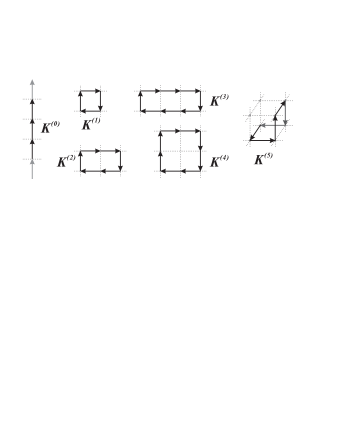
Figure 1: The lattice currents used to determine the transverse elements $f_{i}$ of the monopole action.

coupling	$\eta/\sqrt{\sigma}$	coupling	$\eta/\sqrt{\sigma}$
$f_{0}$	0.521(25)	$f_{1}$	0.577(41)
$f_{2}$	0.565(34)	$f_{3}$	0.544(32)
$f_{4}$	0.554(28)	$f_{5}$	0.591(38)
average: $\mathbf{\eta=0.552(13)\,\sqrt{\sigma}}$

Table 1: The monopole condensate $\eta$ from the fits.

We used $n=6$ extended monopoles to fit of the transverse couplings by functions (6).

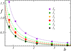
Figure 2: The fits of the monopole couplings.

The fits are shown in Figure 2 and the best fit values of the condensate obtained from the independent fits of couplings $f_{i}$ are presented in Table 1. These values coincide with each other indicating self–consistency of our approach.

Averaging of the results of the six independent fits and taking into account systematic errors we get the value of the monopole condensate, $\eta=243(40)$ MeV. This result is in a quantitative agreement with the value [8], $\eta=194(19)$ MeV, obtained by a completely different method. We conclude that the blocking from continuum is a powerful tool to get the couplings of the DGL model. We are going to get other parameters of the dual model by this method in future [16].

References

- [1] G. ’t Hooft, in High Energy Physics, ed. A. Zichichi, Palermo (1975); S. Mandelstam, Phys. Rept. 23 (1976) 245.
- [2] T. Suzuki, Nucl. Phys. Proc. Suppl. 30 (1993) 176; M. N. Chernodub and M. I. Polikarpov, hep-th/9710205; R.W. Haymaker, Phys. Rept. 315 (1999) 153.
- [3] N. Arasaki et al, Phys. Lett. B 395 (1997) 275; M.Chernodub, M.I.Polikarpov, A.I.Veselov, Phys.Lett.B 399 (1997) 267; Nucl. Phys. Proc. Suppl. 49 (1996) 307; A. Di Giacomo, G. Paffuti, Phys. Rev. D 56 (1997) 6816.
- [4] T. Suzuki, I. Yotsuyanagi, Phys. Rev. D42(1990) 4257; H. Shiba, T. Suzuki, Phys. Lett. B 333 (1994) 461; J. D. Stack, S. D. Neiman, R. J. Wensley, Phys. Rev. D 50 (1994) 3399; G. S. Bali et al, Phys. Rev. D54 (1996) 2863.
- [5] S. Maedan, T. Suzuki, Prog. Theor. Phys. 81 (1989) 229; T. Suzuki, ibid. 81 (1989) 752.
- [6] Y.Matsubara, S.Ejiri, T.Suzuki, Nucl. Phys. Proc. Suppl. 34 (1994) 176; K.Schilling, G.S.Bali, C.Schlichter, ibid. 73 (1999) 638; M.Baker et al, Phys. Rev. D 58 (1998) 034010.
- [7] V. Singh, D. A. Browne, R. W. Haymaker, Phys. Lett. B 306 (1993) 115; see also contribution of T. Matsuki and R. W. Haymaker.
- [8] F.Gubarev et al, Phys.Lett.B 468(1999) 134.
- [9] Y. Koma, M. Koma, E.–M. Ilgenfritz, T. Suzuki, in preparation.
- [10] W.Bietenholz, U.J.Wiese, Nucl.Phys. B464 (1996) 319; Phys.Lett. B 378 (1996) 222; M. N. Chernodub, K. Ishiguro and T. Suzuki, hep-lat/0204003; hep-lat/0202020.
- [11] S. Fujimoto, S. Kato and T. Suzuki, Phys. Lett. B 476, 437 (2000).
- [12] M. N. Chernodub et al, Phys. Rev. D 62 (2000) 094506; hep-lat/9902013.
- [13] T. A. DeGrand, D. Toussaint, Phys. Rev. D 22 (1980) 2478.
- [14] T. L. Ivanenko, A. V. Pochinsky and M. I. Polikarpov, Phys. Lett. B 252 (1990) 631.
- [15] H. Shiba and T. Suzuki, Phys. Lett. B 351 (1995) 519.
- [16] T.Suzuki et al, in preparation.