DESY 03-087

HU-EP-03/39

MS-TP-03-7

SFB/CPP-03-15

Lattice HQET with exponentially improved statistical precision

Michele Della Morte^a, Stephan Dürr^a, Jochen Heitger^b, Heiko Molke^a,

Juri Rolf^c, Andrea Shindler^d and Rainer Sommer^a
a DESY, Zeuthen, Germany ^b Institut für Theoretische Physik, Universität Münster, Münster, Germany ^c Institut für Physik, Humboldt Universität, Berlin, Germany ^d NIC, Zeuthen, Germany
Abstract

We introduce an alternative discretization for static quarks on the lattice retaining the ${\rm O}(a)$-improvement properties of the Eichten-Hill action. In this formulation, statistical fluctuations are reduced by a factor which grows exponentially with Euclidean time, $x_{0}$. For the first time, B-meson correlation functions are computed with good statistical precision in the static approximation for $x_{0}>1\,{\rm fm}$. At lattice spacings $a\approx 0.1\,{\rm fm},\,0.08\,{\rm fm},\,0.07\,{\rm fm}$, the B_s-meson decay constant is determined in the combined static and quenched approximation. A correction due to the finite mass of the b-quark is estimated by interpolating between the static result and a recent determination of $F_{\rm D_{\rm s}}$. Key words: Lattice QCD; Heavy quark effective theory; Static approximation; Modified static actions; B-meson decay constant

PACS: 11.15.Ha; 12.15.Hh; 12.38.Gc; 12.39.Hg; 13.20.He

1. B-physics matrix elements such as the B-meson decay constant $F_{\rm B}$ are obtained from lattice correlation functions at large Euclidean time. Considerable interest lies in the treatment of the b-quark in the leading order of HQET, the static approximation [?,?]: in this framework non-perturbative renormalization can be performed, the continuum limit exists and also $1/m_{{\rm b}}$ corrections can in principle be taken into account [?,?,?,?].

Progress along this line has been hampered by large statistical errors in the static approximation. In particular it has been observed [?] that the errors of a B-meson correlation function roughly grow as

$$R_{\rm NS}\equiv{\rm noise\over\rm signal}\propto\exp\left(x_{0}\,\Delta\right)\,,\;\Delta=E_{\rm stat}-m_{\pi}\,,$$ (1)

where $E_{\rm stat}$ is the ground state energy of a B-meson in the static approximation with the Eichten-Hill action,

$$S_{\rm h}^{\rm EH} = a^{4}\sum_{x}\overline{\psi}_{\rm h}(x)D_{0}\psi_{\rm h}(x)\,,$$ (2)

$$D_{0}\psi_{\rm h}(x) = {1\over a}\,[\psi_{\rm h}(x)-U^{\dagger}(x-a\hat{0},0)\psi_{\rm h}(x-a\hat{0})]\,,$$ (3)

for the static quark [?]. Eq. (1) is problematic because the requirement $R_{\rm NS}\ll 1$ is satisfied only for $x_{0}$ of the order of $\Delta^{-1}$ and this time interval shrinks rapidly to zero in the continuum limit $a\to 0$ where $E_{\rm stat}\sim e_{1}\times g_{0}^{2}/a$ with some number $e_{1}$. In the attempt to eliminate the discretization errors by reducing the lattice spacing, $a$, one is then limited more and more by unwanted contaminations by higher energy states and it has been very difficult to compute matrix elements in the static approximation [?,?,?,?,?]. Since the exponent in eq. (1) is dominated by a divergent term, it is plausible that one may reduce it by changing the discretization. Here we will demonstrate that this is indeed possible while remaining with roughly the same discretization errors.

In [?] it has been shown that energy differences computed with the action eq. (2) are ${\rm O}(a)$-improved if the relativistic sector (light quarks and gluons) is ${\rm O}(a)$-improved. Furthermore, apart from the usual mass dependent factor, $1+b_{\rm A}^{\rm stat}am_{\rm q}$, the static axial current,

$$A^{\rm stat}_{0}(x)=\overline{\psi}_{\rm l}(x)\gamma_{0}\gamma_{5}\psi_{\rm h}(x)\,,$$ (4)

is on-shell ${\rm O}(a)$-improved after adding only one correction term,

$$(A^{\rm stat}_{\rm I})_{0}=A^{\rm stat}_{0}+ac_{\rm A}^{\rm stat}\delta A^{\rm stat}_{0}\,,\quad\delta A^{\rm stat}_{0}(x)=\overline{\psi}_{\rm l}(x)\gamma_{j}\gamma_{5}{{\overleftarrow{\nabla}_{j}}+\overleftarrow{\nabla}\kern-0.5pt\smash{\raise 4.5pt\hbox{$\ast$}}\kern-4.5pt_{j}\over 2}\psi_{\rm h}(x)\,.$$ (5)

We want to retain these properties of the theory. They are guaranteed if the lattice Lagrangian is invariant under the following symmetry transformations (we do not list the usual ones such as parity and cubic invariance) [?].

• Heavy quark spin symmetry:

  $$\psi_{\rm h}\longrightarrow{\cal V}\psi_{\rm h}\,,\qquad\overline{\psi}_{\rm h}\longrightarrow\overline{\psi}_{\rm h}{\cal V}^{-1}\,,\quad{\rm with}\quad{\cal V}=\exp(-i\phi_{i}\epsilon_{ijk}\sigma_{jk})\,.$$ (6)

• Local conservation of heavy quark flavor number:

  $$\psi_{\rm h}\longrightarrow{\rm e}^{i\eta({\it\bf x})}\,\psi_{\rm h}\,,\qquad\overline{\psi}_{\rm h}\longrightarrow\overline{\psi}_{\rm h}{\rm e}^{-i\eta({\it\bf x})}.$$ (7)

Keeping these symmetries intact, there is little freedom to modify the action. We may, however, alter the way the gauge fields enter the discretized covariant derivative, $D_{0}$. To this end we choose

$$D_{0}\psi_{\rm h}(x)={1\over a}\,[\psi_{\rm h}(x)-W^{\dagger}(x-a\hat{0},0)\,\psi_{\rm h}(x-a\hat{0})]\,,$$ (8)

with $W(x,0)$ a generalized gauge parallel transporter with the gauge transformation properties of $U(x,0)$. In particular we take $W(x,0)$ to be a function of the link variables in the neighborhood of $x$, which is invariant under spatial cubic rotations and does have the correct classical continuum limit such that $D_{0}=\partial_{0}+A_{0}+{\rm O}(a^{2})$. This is enough to ensure that the universality class as well as ${\rm O}(a)$-improvement are unchanged in comparison to eq. (3). Since we expect the size of remaining higher order lattice artifacts to be moderate if one keeps the action rather local, we here consider only choices where $W(x,0)$ is a function of gauge fields in the immediate neighborhood of $x,x+a\hat{0}$. We choose

$$W_{\rm S}(x,0) = V(x,0)\,\left[{g_{0}^{2}\over 5}+\Big{(}{1\over 3}\,\hbox{tr}\,V^{\dagger}(x,0)V(x,0)\Big{)}^{1/2}\right]^{-1}\,,$$ (9)

$$W_{\rm A}(x,0) = V(x,0)\,,$$ (10)

$$W_{\rm HYP}(x,0) = V_{\rm HYP}(x,0)\,,$$ (11)

where

$$V(x,0)={1\over 6}\sum_{j=1}^{3} [ U(x,j)U(x+a\hat{j},0)U^{\dagger}(x+a\hat{0},j)$$ (12)

$$+\,U^{\dagger}(x-a\hat{j},j)U(x-a\hat{j},0)U(x+a\hat{0}-a\hat{j},j)\,\,\,\,]\,,$$

and where the so-called HYP-link, $V_{\rm HYP}(x,0)$, is a function of the gauge links located within a hypercube [?,?]. In the latter case we take the parameters $\alpha_{1}=0.75$, $\alpha_{2}=0.6$, $\alpha_{3}=0.3$ [?]. The choices (9) – (11) will be motivated further in [?]. It is worth pointing out that a covariant derivative of the general type used above has first been introduced in [?]. In this reference it was considered for the Kogut-Susskind action for relativistic quarks and with a different motivation.

2. Next we have to study the scaling behaviour of observables computed with the actions $S_{\rm h}^{\rm S},\,S_{\rm h}^{\rm A},\,S_{\rm h}^{\rm HYP}$ which are obtained by inserting $W_{\rm S},\,W_{\rm A},\,W_{\rm HYP}$ into eqs. (8) and (2). In [?] this scaling behaviour is analyzed in depth for various observables and various choices for the static action in perturbation theory and non-perturbatively. Here we will present only one example. The necessity of such an investigation can be underlined by the following consideration.

The static potential can be seen as an energy for a static quark with action $S_{\rm h}$ and an antiquark with the corresponding $S_{\bar{\rm h}}$ [?]. Hence, the static force is one indicator for the scaling behavior of these actions. In [?], rather large $a^{2}$-effects have been seen in the short-distance force for $S_{\rm h}^{\rm HYP}$ and $S_{\bar{\rm h}}^{\rm HYP}$.

One may therefore worry about large $a$-effects, in particular in correlation functions of the static-light axial current, where static and light quarks propagate also close to each other. With the new actions, $A^{\rm stat}_{0}$ is ${\rm O}(a)$-improved once [?]

$$c_{\rm A}^{\rm stat} = -0.08237\,g_{0}^{2}+{\rm O}(g_{0}^{4})\,,\quad\mbox{for}\;S_{\rm h}=S_{\rm h}^{\rm EH}\,,$$ (13)

$$c_{\rm A}^{\rm stat} = 0.0072(4)\,g_{0}^{2}+{\rm O}(g_{0}^{4})\,,\quad\mbox{for}\;S_{\rm h}=S_{\rm h}^{\rm S},S_{\rm h}^{\rm A}\,,$$ (14)

$$c_{\rm A}^{\rm stat} = 0.0385(37)\,g_{0}^{2}+{\rm O}(g_{0}^{4})\,,\quad\mbox{for}\;S_{\rm h}=S_{\rm h}^{\rm HYP}\,,$$ (15)

is set in eq. (5). The improvement coefficient $b_{\rm A}^{\rm stat}$ is set to its tree–level value $b_{\rm A}^{\rm stat}=1/2$ in this work.

We consider now a step scaling function, $\Sigma_{\rm A}^{\rm stat}$, which gives the change of the renormalized static axial current in a Schrödinger functional (SF) scheme [?], when the renormalization scale is changed from $\mu=1/L$ to $\mu=1/(2L)$. Its continuum limit is known for a few values of $L$ [?]. This quantity is thus a good observable to search for $a$-effects. In Fig. 1 we show $\Sigma_{\rm A}^{\rm stat}(3.48,a/L)$, where the first

Figure 1: The step scaling function $\Sigma_{\rm A}^{\rm stat}(3.48,a/L)$ for different choices of the action $S_{\rm h}$. Results for $S_{\rm h}^{\rm EH}$ were extrapolated to $\Sigma_{\rm A}^{\rm stat}(3.48,0)$ [?] ($\bullet$). In all cases $c_{\rm A}^{\rm stat}$ from 1-loop perturbation theory is used, which is sufficient since $\Sigma_{\rm A}^{\rm stat}(3.48,a/L)$ does not depend very sensitively on this improvement coefficient. For $S_{\rm h}^{\rm A}$, $S_{\rm h}^{\rm S}$ and $S_{\rm h}^{\rm HYP}$ points have been displaced on the horizontal axis for clarity.

argument parameterizes $L$ in terms of the SF-coupling $\bar{g}^{2}(L)=3.48$. ${\rm O}(a)$-improvement is employed as in [?] but we consider the different actions for the static quark introduced above. All of them lead to $\Sigma_{\rm A}^{\rm stat}(3.48,a/L)$ at finite $a/L$ differing from the continuum limit by about the same amount. Supported also by further such studies [?], we conclude that within the set of actions studied none is particularly distinguished by its scaling behavior.

3. Let us now demonstrate that the statistical errors at large Euclidean time are reduced by the choices eqs. (9) – (11). As a B-meson correlation function we choose

$$f_{\rm A}^{\rm stat}(x_{0},\omega)=-\hbox{$1\over 2$}\langle(A^{\rm stat}_{\rm I})_{0}(x)\,{\mathcal{O}}(\omega)\rangle\,,\quad{\mathcal{O}}(\omega)={a^{6}\over L^{3}}\sum_{{\it\bf y},{\it\bf z}}\overline{\zeta}_{\rm h}({\it\bf y})\gamma_{5}\omega({\it\bf y}-{\it\bf z}){\zeta_{\rm l}}({\it\bf z})\,,$$ (16)

defined in the Schrödinger functional with $T=3L/2$, $L/a=24$, $\beta=6/g_{0}^{2}=6.2$ and a vanishing background field [?]. Here, as a novelty compared to previous applications, a wave function $\omega({\it\bf x})$ is introduced to construct an interpolating B-meson field in terms of the boundary quark fields ${\zeta_{\rm l}}$ and $\overline{\zeta}_{\rm h}$. It may be exploited to reduce the contribution of excited B-meson states to the correlation function, but this does not concern us yet. At the moment we simply consider $\omega({\it\bf x})=1$ and form the ratio $R_{\rm NS}$, eq. (1), for the different actions. From now on we set the light quark mass to the strange quark mass, taken from [?] following exactly [?] concerning the technical details. Figure 2 shows that in all

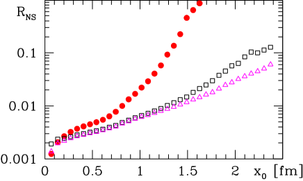
Figure 2: The ratio $R_{\rm NS}$, eq. (1), for the correlation function $f_{\rm A}^{\rm stat}$ for a statistics of 2500 measurements. Circles refer to $S_{\rm h}^{\rm EH}$ while squares and triangles to $S_{\rm h}^{\rm S}$ and $S_{\rm h}^{\rm HYP}$, respectively. $S_{\rm h}^{\rm A}$ behaves like $S_{\rm h}^{\rm S}$. Physical units are set by using $r_{0}=0.5\,{\rm fm}$ [?,?].

cases $R_{\rm NS}$ grows exponentially with $x_{0}$. For the Eichten-Hill action, also the effective coefficient $\Delta$, describing the growth for $x_{0}=1\,{\rm fm}-2\,{\rm fm}$, is roughly given by $E_{\rm stat}-m_{\pi}$ in agreement with eq. (1), while for the other actions this is not the case. Most importantly for the other actions, $\Delta$ is reduced by a factor around 4, and with the statistics in our example a distance of $x_{0}\approx 2\,{\rm fm}$ is reached with $S_{\rm h}^{\rm HYP}$ if one requires $R_{\rm NS}\leq 2\%$. The actions $S_{\rm h}^{\rm A},S_{\rm h}^{\rm S}$ behave only slightly worse.

4. This reduction of statistical errors enables us to choose $\omega({\it\bf x})$ such that a long and precise plateau is visible in the effective energy,

$$E_{\rm eff}(x_{0},\omega)=\ln\left[f_{\rm A}^{\rm stat}(x_{0}-a,\omega)/f_{\rm A}^{\rm stat}(x_{0}+a,\omega)\right]/(2a)\,,$$ (17)

as shown in Fig. 3.

Figure 3: Effective energies for wave functions $\Omega_{1}$ (open symbols) and $\Omega_{2}$ (filled symbols) using $S_{\rm h}^{\rm HYP}$ (circles) and $S_{\rm h}^{\rm S}$ (triangles). Results refer to a $24^{3}\times 36$ lattice, $\beta=6.2$.

Neither position nor length of the plateau depend sensitively on the details of $\omega$, as long as it is chosen such that the first excited state in the B-meson channel is canceled to a good approximation. For the figure as well as for the following, we have chosen $\omega\in\{\Omega_{1},\Omega_{2}\}$ with

$$\Omega_{1} = \omega_{1}+\alpha\omega_{3}\,,\quad\Omega_{2}=\omega_{2}+\alpha^{\prime}\omega_{4}\,,$$ (18)

$$\omega_{i}({\it\bf x}) = N_{i}^{-1}\sum_{{\bf n}\in{\bf Z}^{3}}\overline{\omega}_{i}(|{\it\bf x}-{\bf n}L|)\,,\;i=1,2,3\,,$$

$$\overline{\omega}_{1}(r) = r_{0}^{-3/2}\,{\rm e}^{-r/a_{0}}\,,\quad\overline{\omega}_{2}(r)=r_{0}^{-3/2}\,{\rm e}^{-r/(2a_{0})}\,,\quad\overline{\omega}_{3}(r)=r_{0}^{-5/2}\,r\,{\rm e}^{-r/(2a_{0})}\,,$$

$$\omega_{4}({\it\bf x}) = L^{-3/2}\,,$$ (19)

where $a_{0}=0.1863\,r_{0}$ and the (dimensionless) coefficients $N_{i}$ are chosen such that $a^{3}\sum_{\bf x}\omega_{i}^{2}({\bf x})=1$. The B-meson decay constant is then obtained from the renormalization group invariant matrix element [?]

$$\Phi_{{\rm RGI}}(x_{0})=-Z_{\rm RGI}\,(1+b_{\rm A}^{\rm stat}am_{\rm q})\,2L^{3/2}{{f_{\rm A}^{\rm stat}(x_{0})}\over{\sqrt{f_{1}(T^{\prime},\omega)}}}\,{\rm e}^{(x_{0}-T^{\prime}/2)E_{\rm eff}(x_{0})}$$ (20)

of the static axial current, where

$$f_{1}(T,\omega)=-\hbox{$1\over 2$}\langle{\mathcal{O}}^{\prime}(\omega){\mathcal{O}}(\omega)\rangle\,,\quad{\mathcal{O}}^{\prime}(\omega)={a^{6}\over L^{3}}\sum_{{\it\bf y},{\it\bf z}}\overline{\zeta}_{\rm l}\kern 1.0pt^{\prime}({\it\bf y})\gamma_{5}\,\omega({\it\bf y}-{\it\bf z})\zeta_{\rm h}\kern 1.0pt^{\prime}({\it\bf z})\,.$$ (21)

The renormalization factor, $Z_{\rm RGI}$, relates the bare matrix element to the renormalization group invariant one [?]. Its regularization dependent part is computed exactly as in that reference, but for the new actions. In Table 1 we give results for $\Phi_{{\rm RGI}}(x_{0})$ for three values of the lattice spacing and selected choices of $T,T^{\prime},x_{0}$, highlighting what we selected for further analysis. These numbers do not change significantly if we vary the improvement coefficients $c_{\rm A}^{\rm stat}$ and $b_{\rm A}^{\rm stat}$, which are known only in perturbation theory, by factors of two. We thus extrapolate our results quadratically in the lattice spacing and arrive at our estimate for the continuum limit

$$r_{0}^{3/2}\Phi_{{\rm RGI}}=1.78(13)\,.$$ (22)

						$\Omega_{1}$	$\Omega_{2}$
$\beta$	$a\,[{\rm fm}]$	$L/a$	$T/a$	$T^{\prime}/a$	$x_{0}/a$	$r_{0}^{3/2}\Phi_{{\rm RGI}}$		$\alpha$	$\alpha^{\prime}$
6.0	0.093	16	24	24	12	1.830(31)	1.832(30)	0.278	$-0.200$
6.0	0.093	16	24	20	12	1.847(18)	1.830(17)	0.278	$-0.200$
6.0	0.093	16	24	24	10	1.818(31)	1.828(30)	0.278	$-0.200$
6.0	0.093	16	24	20	10	1.851(17)	1.829(17)	0.278	$-0.200$
6.1	0.079	24	30	30	15	1.864(56)	1.858(52)	0.756	0.022
6.1	0.079	24	30	30	12	1.850(56)	1.846(52)	0.756	0.022
6.2	0.068	24	36	36	18	1.724(78)	1.760(75)	0.351	$-0.176$
6.2	0.068	24	36	36	15	1.726(78)	1.763(76)	0.351	$-0.176$

Table 1: Decay constant in static approximation.

5. The result eq. (22) may be used to compute $F_{\rm B_{\rm s}}$ by taking account of the mass dependent function [?] $C_{\text{PS}}(M_{\text{b}}/\Lambda_{\overline{\rm MS}})=F_{\rm B}\sqrt{m_{\text{B}}}/\Phi_{{\rm RGI}}=1.22(3)$, evaluated using the 3-loop anomalous dimension [?] and the associated matching coefficient between HQET and QCD [?]. $M_{\rm b}$ denotes the renormalization group invariant b-quark mass [?,?]. With this we arrive at $r_{0}F_{\rm B_{\rm s}}^{\text{stat}}=0.57(4)$. A correction due to the finite mass of the b-quark can be computed by connecting the static result eq. (22) and

$$r_{0}^{3/2}{{F_{\rm D_{s}}\sqrt{m_{\rm D_{s}}}}\over{C_{\rm PS}(M_{\rm c}/\Lambda_{\overline{\rm MS}})}}=1.33(7)$$ (23)

by a linear interpolation in the inverse meson mass. Here we have used recent computations of the D${}_{\text{s}}$-meson decay constant [?] and of the charm quark mass [?]. In this way we obtain

$$r_{0}F_{\rm B_{\rm s}}=0.52(3)\to F_{\rm B_{\rm s}}=205(12)\,{\rm MeV}\;\mbox{with}\;r_{0}=0.5\,{\rm fm}\,.$$ (24)

Conservatively, we may attribute an additional $\approx 5\,\%$ uncertainty to the fit ansatz used, but our personal estimate is that this error is significantly smaller and it will soon be quantified [?].

One should remember that eq. (24) refers to the quenched approximation and as in [?] a $12\,\%$ scale ambiguity may be estimated from the slope of the linear interpolation.

6. An interesting point is that the potential in full QCD may be computed replacing the time-like links in the Wilson loop (or Polyakov loops) by the different $W_{i}$ introduced above. In particular the “HYP-link potential” [?] may be used. Depending on which $W_{i}$ is chosen, the static potentials differ from each other, but all of them approach the continuum limit with ${\rm O}(a^{2})$ corrections if the action used for the dynamical fermions is ${\rm O}(a)$-improved. This property follows from the considerations of [?] applied to the static actions introduced above, which satisfy all the necessary requirements. This virtue of e.g. the HYP-link potential was not obvious before. Using it, better precision can be reached and some signs of string breaking [?] may become visible.

7. To summarize, we have shown that a modification of the Eichten-Hill static action can be found which keeps lattice artifacts in heavy-light correlation functions moderate but reduces statistical errors to a level making the region $x_{0}>1.5\,{\rm fm}$ accessible. Furthermore, the new action can be used without change for dynamical fermions and also to compute the static potential with dynamical fermions. As a demonstration of the usefulness of this reduction of statistical errors, we have computed $F_{\rm B_{\rm s}}$ in the quenched approximation, by joining the continuum limit of the static approximation estimated with the new action with the previously determined continuum limit of $F_{\rm D_{\rm s}}$ by means of a linear interpolation. This procedure can systematically be improved by computing 1) the mass dependence around $m_{{\rm c}}$, 2) the $1/m$ corrections to the static limit and 3) repeating the whole analysis with dynamical fermions. Work along these lines is in progress and a more detailed investigation of the properties of various static quark actions is in preparation.

Acknowledgments. We are grateful to M. Lüscher and F. Knechtli for comments on the manuscript. We thank DESY for allocating computer time on the APEmille computers at DESY Zeuthen to this project and the APE-group for its valuable help. This work is also supported by the EU IHP Network on Hadron Phenomenology from Lattice QCD under grant HPRN-CT-2000-00145 and by the Deutsche Forschungsgemeinschaft in the SFB/TR 09.

References

- [1] E. Eichten, Talk delivered at the Int. Sympos. of Field Theory on the Lattice, Seillac, France, Sep 28 - Oct 2, 1987.
- [2] E. Eichten and B. Hill, Phys. Lett. B234 (1990) 511.
- [3] ALPHA, M. Kurth and R. Sommer, Nucl. Phys. B597 (2001) 488, hep-lat/0007002.
- [4] ALPHA, J. Heitger and R. Sommer, Nucl. Phys. Proc. Suppl. 106 (2002) 358, hep-lat/0110016.
- [5] R. Sommer, (2002), hep-lat/0209162.
- [6] J. Heitger, M. Kurth and R. Sommer, (2002), hep-lat/0209078.
- [7] S. Hashimoto, Phys. Rev. D50 (1994) 4639, hep-lat/9403028.
- [8] C.R. Allton et al., Nucl. Phys. B349 (1991) 598.
- [9] C. Alexandrou et al., Phys. Lett. B256 (1991) 60.
- [10] A. Duncan et al., Phys. Rev. D51 (1995) 5101, hep-lat/9407025.
- [11] R. Sommer, Phys. Rept. 275 (1996) 1, hep-lat/9401037.
- [12] A. Hasenfratz and F. Knechtli, Phys. Rev. D64 (2001) 034504, hep-lat/0103029.
- [13] A. Hasenfratz, R. Hoffmann and F. Knechtli, Nucl. Phys. Proc. Suppl. 106 (2002) 418, hep-lat/0110168.
- [14] M. Della Morte, A. Shindler and R. Sommer, in preparation.
- [15] T. Blum et al., Phys. Rev. D55 (1997) 1133, hep-lat/9609036.
- [16] S. Necco and R. Sommer, Nucl. Phys. B622 (2002) 328, hep-lat/0108008.
- [17] J. Heitger, M. Kurth and R. Sommer, (2003), hep-lat/0302019.
- [18] ALPHA, J. Garden et al., Nucl. Phys. B571 (2000) 237, hep-lat/9906013.
- [19] ALPHA, J. Rolf and S. Sint, JHEP 12 (2002) 007, hep-ph/0209255.
- [20] R. Sommer, Nucl. Phys. B411 (1994) 839, hep-lat/9310022.
- [21] ALPHA, M. Guagnelli, R. Sommer and H. Wittig, Nucl. Phys. B535 (1998) 389, hep-lat/9806005.
- [22] ALPHA, M. Guagnelli et al., Nucl. Phys. B560 (1999) 465, hep-lat/9903040.
- [23] K.G. Chetyrkin and A.G. Grozin, (2003), hep-ph/0303113.
- [24] D.J. Broadhurst and A.G. Grozin, Phys. Rev. D52 (1995) 4082, hep-ph/9410240.
- [25] ALPHA, A. Jüttner and J. Rolf, Phys. Lett. B560 (2003) 59, hep-lat/0302016.
- [26] ALPHA, in preparation .
- [27] K. Schilling, Nucl. Phys. Proc. Suppl. 83 (2000) 140, hep-lat/9909152.