CERN-TH/2003-154
MIT-CTP-3395
{centering}
The QCD Phase Diagram for Three Degenerate Flavors and Small Baryon Density
Philippe de Forcranda,b and Owe Philipsenc
a
Institut für Theoretische Physik,
ETH Zürich,
CH-8093 Zürich,
Switzerland
b
Theory Division, CERN, CH-1211 Geneva 23,
Switzerland
c
Center for Theoretical Physics, Massachusetts Institute of Technology,
Cambridge, MA 02139-4307, USA
We present results for the phase diagram of three flavor QCD for MeV. Our simulations are performed with imaginary chemical potential for which the fermion determinant is positive. Physical observables are then fitted by truncated Taylor series and continued to real chemical potential. We map out the location of the critical line with an accuracy up to terms of order . We also give first results on a determination of the critical endpoint of the transition and its quark mass dependence. Our results for the endpoint differ significantly from those obtained by other methods, and we discuss possible reasons for this.
1 Introduction
The last two years have seen significant progress in simulating QCD at small baryon densities. Standard Monte Carlo methods fail in the presence of a non-vanishing chemical potential, for which the fermion determinant is complex and prohibits importance sampling with positive weights. While this problem remains unsolved for QCD, there are presently three avenues to investigate the -phase diagram, as long as the quark chemical potential in units of temperature, , is sufficiently small: A two-dimensional generalization of the Glasgow method [1] predicts a phase diagram with a first order phase transition at large , terminating in a critical endpoint [2]. Taylor expanding the observables and the reweighting factor leads to coefficients expressed in local operators and thus permits the study of larger volumes [3]. Simulations at imaginary chemical potential are not limited in volume since the fermion determinant is positive. They allow for fits of the full observables by truncated Taylor series, thus controlling the convergence of the latter, and subsequent analytic continuation to real [4].
The results for the location of the pseudo-critical line are consistent among all three approaches for baryon chemical potentials up to MeV (). This latter number gives the range of applicability of method , and hence the range over which convergence of the Taylor series can be checked explicitly. A review comparing these methods in detail can be found in [5]. However, the location of the endpoint of the phase transition has only been computed by one method and for one set of quark masses [2]. Since the numerical study of critical phenomena is notoriously difficult even for , it is important to cross-check this result by another method.
In the present paper we investigate QCD with three degenerate quark flavors by lattice simulations with imaginary chemical potential. In this case we know reasonably well the chiral critical point , i.e. the critical bare quark mass for which the deconfinement transition changes from first order to crossover [6, 7, 8]. This point marks a second order phase transition in the universality class of the 3d Ising model [7]. For the -phase diagram this means that for the line of first order deconfinement/chiral phase transitions extends all the way to the temperature axis at , whereas for it terminates at a critical point . The critical chemical potential, , is expected to grow with the quark mass. Inverting this relation yields the change in the critical bare quark mass with chemical potential, . Our goal is to determine this function for chemical potentials MeV.
We begin by computing the quark mass and chemical potential dependence of the critical line, . Our simulations are accurate enough to allow for a determination of the coefficient of its Taylor series. We then proceed to extract by measuring the Binder cumulant of the chiral condensate. We find the -dependence of the latter to be very weak, proving a quantitative determination of to be extremely difficult. Just like the critical temperature, is an even function of the chemical potential with a Taylor expansion in . We are only able to determine the first non-trivial coefficient with an error of 40%. However, this allows us to give a conservative upper bound on this coefficient at the 90% confidence level. This bound is in disagreement with a preliminary result obtained by Taylor expanded reweighting [15].
After summarizing the imaginary chemical potential approach in Sec. 2, Sec. 3 discusses general qualitative features and expectations about the three flavor phase diagram and how it can be determined by simulations at imaginary chemical potential. Sec. 4 introduces the Binder cumulant and its finite volume scaling as our computational tool to determine the order of the phase transition as a function of quark mass and chemical potential. Our numerical results are presented in Sec. 5, followed by a discussion and comparison with other work in Sec. 6. Finally, we give our conclusions.
2 The QCD phase transition from imaginary
This section serves to fix the notation and summarize what is needed in the sequel. For a detailed discussion of the formalism we refer to [4]. The QCD grand canonical partition function , with the same chemical potential for all flavors, can be considered for complex chemical potential . Two general symmetry properties can be used to constrain the phase structure of the theory as a function of : is an even function of , , where ; A non-periodic gauge transformation, which rotates the Polyakov loop by a center element but leaves unchanged, is equivalent to a shift in [9]:
| (1) |
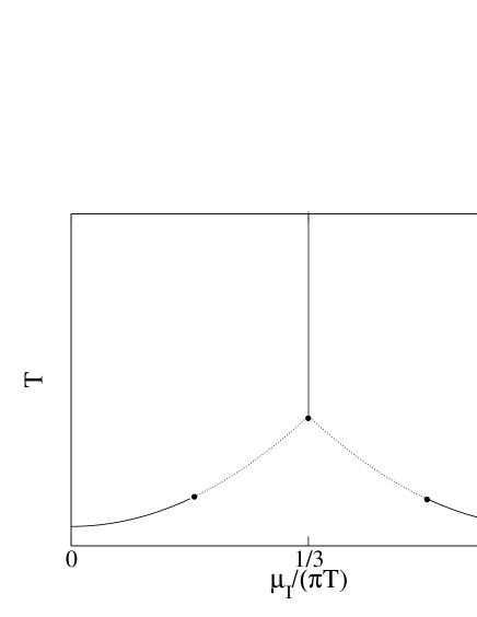
For QCD (), these two properties lead to transitions at critical values of the imaginary chemical potential, , separating regions of parameter space where the Polyakov loop angle falls in different sectors. The resulting phase diagram in the plane is periodic and symmetric about , as depicted in Fig. 1 for . The transitions are first order for high temperatures, terminating at some critical temperature which coincides with the deconfinement line. This endpoint also belongs to the 3d Ising universality class [4]. The curves in Fig. 1 correspond to the deconfinement line continued to imaginary chemical potential, . We will map out these curves as well as the location of the critical endpoint as a function of quark mass. Their relation to real is discussed in detail in the next section.
On the lattice, phase transitions can be studied by measuring fluctuations of gauge invariant operators,
| (2) |
where we use the plaquette, the chiral condensate and the modulus of the Polyakov loop for . A transition region is signalled by a peak in the susceptibilities
| (3) |
whose maximum implicitly defines the critical parameters, . In a finite volume, the susceptibility is always an analytic function of the parameters of the theory, even in the presence of a phase transition. The latter reveals itself by a divergence of in the infinite volume limit, whereas stays finite in the case of a crossover. This fact was used in [4] to show that, on any large but finite volume, the pseudo-critical coupling can be represented by a Taylor series in . Here we also wish to study the quark mass dependence, and thus consider an additional expansion in about the chiral critical point . Hence we have for the pseudo-critical coupling on a finite volume
| (4) |
With the help of the two-loop lattice beta-function, the critical coupling can be converted to the critical temperature . In our previous work [4] we demonstrated by simulations that the -series converges fast and the critical coupling viz. temperature are well described by the leading -term. Analytic continuation between real and imaginary chemical potential is then trivial.
Following [10, 11, 4], our strategy thus consists of measuring observables at , fitting them by a Taylor series in and then continuing the truncated Taylor series to real . The -transition closest to the origin, at , defines the convergence radius of the expansion and limits the prospects of analytic continuation. In physical units this corresponds to MeV.
3 Qualitative features of the phase diagram
In principle, as proposed in [4], the order of the phase transition, and hence the location of the critical point, can be determined from a finite size scaling analysis of the critical coupling itself, which attains its infinite volume limit as
| (5) |
where for a first order phase transition, for a second order phase transition, and for a crossover. The critical endpoint on the curve is then defined by , for which the transition is of second order. However, such an analysis is not practical for analytic continuation. In a Taylor expansion in , the volume dependence resides in the coefficients,
| (6) |
Clearly, a -dependent finite volume behavior as in Eq. (5) cannot in general be well approximated by only a few terms of this series.
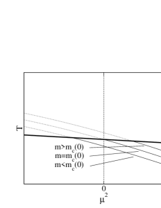
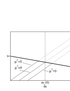
Fortunately, the problem can be approached differently by considering variations of the quark mass, as outlined in [12]. In this case we have a three-dimensional parameter space . The critical temperature now describes a surface in this space, and the critical endpoint traces out a line , or equivalently , on this surface. Projections of this situation onto the and -planes are shown schematically in Fig. 2 and 3. The bottom line in Fig. 2 (left) corresponds to the situation depicted in Fig. 1, for some quark mass . With increasing quark mass, the critical endpoint of the deconfinement line in Fig. 1 moves towards , which it hits for . On the other hand, for decreasing quark mass it moves to larger , until it meets the endpoint at some mass . For the deconfinement and transition lines are connected.
This feature appears in Fig. 3 as the intersection of with the vertical -line, which can be shown as follows. In the chiral limit, the chiral condensate represents a true order parameter which is strictly zero in the deconfined phase, and there must be a true phase transition for all values . Thus the line separating first order from crossover, , cannot hit the negative -axis unless it has an unexpected non-analyticity there, implying the existence of some .
Since the (pseudo-) critical line is analytic, so is the line of endpoints , and by elimination of the same holds for . These are again smooth functions with analytic continuations to imaginary , which one may hope to describe well in terms of only a few coefficients. In our practical calculation we attempt to map out the phase diagram Fig. 3 by computing the coefficients of
| (7) |
Preliminary results for the leading coefficient as determined from Taylor expanded reweighting, have been reported in [13], and we will discuss this result in comparison to ours in Sec. 6.
3.1 Theoretical expectations
Before continuing to describe our calculational tools, let us make a few remarks about what one would expect theoretically. The analytic continuation approach has by now been tested for screening masses in the plasma phase [11] as well as for [4, 14]. In [11] it was remarked that the screening masses are most “naturally” expanded in , where “natural” means that the coefficients in such a series are of order one. The same observation is made regarding the critical temperature for the two flavor case. The result quoted in [4] can be rewritten as
| (8) |
where the coefficient is of order one. In thermal perturbation theory this is easy to understand, as in the imaginary time formalism one expands in terms of Matsubara modes and the chemical potential always appears in this combination [11, 17]. It is also transparent non-perturbatively in the case of an imaginary chemical potential : the chemical potential gives an extra factor for the boundary condition on the fermionic fields, so that it is equivalent to shifting the Matsubara frequencies by . Hence the relevant expansion parameter is the relative shift . We will empirically confirm this for the three flavor case, where we also measure the next-to-leading coefficient.
The same considerations apply to the quark mass expansion and provide a reason for the near independence of upon the light quark masses [3]. Fermionic modes contribute with non-zero Matsubara frequencies, and light quark masses are always negligible compared to those modes, . This is still the case for the strange quark mass, and so we expect the curve to be approximately the same for and .
For the critical quark mass one then similarly expects to have
| (9) |
with of order one. The bare quark mass is not a physical quantity, but depends on the lattice action. For example, comparing calculations with p4-improved and unimproved staggered fermion actions, one finds [7]. However, the mass renormalization should not be affected by , which is just an external thermodynamic parameter without ultraviolet renormalization. Multiplicative mass renormalization should therefore cancel out in the ratio Eq. (9), which, up to additive corrections , is directly comparable between different lattice actions.
A remarkable finding for the critical temperature is that it is quite accurately described by the leading term, at least up to , where for imaginary the transition occurs. The same was found for screening masses [11] and recently also for the pressure [15]. We thus expect similar behavior for , which will be confirmed by our simulations. If is well described by the leading term, its intersection with the -line at a quark mass value , as described in the previous section, furthermore implies an upper bound for . From Eq.(9) one gets , or .
4 Cumulant ratio and finite volume scaling
In order to find the boundary between the first order and crossover regime along the critical line, we use the Binder cumulant [16] of the chiral condensate,
| (10) |
In the infinite volume limit this quantity assumes a universal value at a critical point. In particular, this observable was used in [7] to locate the chiral critical point at , for staggered fermions on an lattice, and to identify its universality class as that of the 3d Ising model, for which . On a finite volume, this value receives corrections. It also receives corrections away from the critical point, which are positive for crossover and negative for first order behavior. Cumulants calculated on increasing lattice sizes for different parameters will intersect at some pseudo-critical value of the parameters, with the -value at the intersection point converging towards its universal value.
In order to explicitly assess the quark mass and -dependence, we fit our data by a Taylor expansion about the critical point,
| (11) |
with . This observable can also be directly related to the critical line in the phase diagram Fig. 3. At the expansion point we have , and this value is maintained along the line , which is a line of constant . This line is implicitly defined by the equation
| (12) |
and in particular one obtains the coefficient of Eq. (9) through the chain rule
| (13) |
If the volumes are large enough, the approach to the thermodynamic limit is governed by universality. In this case the volume dependence hidden in the coefficients of the series can be made explicit. Approaching the critical endpoint, the correlation length diverges as , where is the distance to the critical point in the plane of temperature and magnetic field-like variables, and for the Ising universality class. In practice, we first find for a given pair , and then compute for those values of the couplings. Since always, we thus have . is a function of the dimensionless ratio , or equivalently . Hence one expects the scaling behavior
| (14) |
5 Numerical results
In our simulations we consider QCD with the Wilson gauge action and three degenerate flavors of staggered fermions, with bare quark masses in the range . We monitor finite volume scaling behavior using three lattice sizes, , and . The Monte Carlo employs the R-algorithm [18] with a step size , which is sufficiently small for the systematic errors to be negligible compared to our statistical errors. For each simulated parameter set we accumulate unit-length trajectories, measuring the gauge action and the Polyakov loop and estimating the first four powers of the chiral condensate after each trajectory. The pseudo-critical values are obtained from a range of typically simulated -values by means of the Ferrenberg-Swendsen reweighting method [19]. Hence, every data point in the following figures for the critical coupling and the cumulant ratio typically consists of over trajectories.
5.1 The critical line
The calculation of the critical line proceeds as in the two flavor case [4]. The critical coupling was determined by finding a peak in the plaquette susceptibility, and we have checked that the chiral condensate and the Polyakov loop give consistent results. Our first task then is to determine the coefficients in the Taylor expansion Eq. (4).
In Table 1 we give an exhaustive list of all possible three, four and six parameter fits to our data. For the expansion point in the quark mass, we have chosen , which will be the result obtained in Sec. 5.3. Apart from resolving the leading linear quark mass and quadratic chemical potential dependence, our statistics is now also large enough to permit some statements concerning the next-to-leading terms. On our lattice we studied the largest , and consequently get the most constrained fits for the -term. Note that on this volume a quartic term is required to fit the data, while the other possibilities give significantly worse fits. The situation on the other volumes is consistent with this. The best four parameter fit is in all cases the one with a -term. The other options give coefficients that are either consistent with zero within 1.5 standard deviations, or inconsistent between the different volumes. On the other hand, six parameter fits do not significantly reduce the , and thus are not fully constrained yet.
Comparing the coefficients of the fits including the quartic term between the volumes, we observe that the present statistics is unable to resolve systematic finite volume effects, all volumes being compatible within one standard deviation. It is then expedient to further constrain the fit parameters by fitting all volumes together. We use the best four parameter fit highlighted in the table as our final result for the critical coupling, which is shown in Fig. 4 as a function of .
| 8 | 5. | 1450(2) | 0. | 790(8) | – | 1. | 748(26) | – | – | 0. | 94 | |||
|---|---|---|---|---|---|---|---|---|---|---|---|---|---|---|
| 8 | 5. | 1451(2) | 0. | 739(26) | 0. | 93(46) | 1. | 735(27) | – | – | 0. | 66 | ||
| 8 | 5. | 1449(3) | 0. | 791(8) | – | 1. | 745(27) | 2. | 3(6.3) | – | 1. | 01 | ||
| 8 | 5. | 1450(2) | 0. | 789(8) | – | 1. | 751(31) | – | -0. | 085(0.40) | 1. | 02 | ||
| 8 | 5. | 1449(4) | 0. | 740(27) | 0. | 99(48) | 1. | 712(44) | 6. | 8(9.9) | 0. | 38(0.63) | 0. | 75 |
| 10 | 5. | 1449(2) | 0. | 800(5) | – | 1. | 831(23) | – | – | 7. | 66 | |||
| 10 | 5. | 1457(2) | 0. | 667(15) | 1. | 98(22) | 1. | 818(23) | – | – | 1. | 21 | ||
| 10 | 5. | 1457(2) | 0. | 798(5) | – | 1. | 808(23) | -28. | 2(4.6) | – | 5. | 41 | ||
| 10 | 5. | 1449(2) | 0. | 798(5) | – | 1. | 883(40) | – | -0. | 38(25) | 8. | 04 | ||
| 10 | 5. | 1458(2) | 0. | 679(17) | 1. | 78(25) | 1. | 820(42) | -8. | 6(5.6) | -0. | 07(26) | 1. | 21 |
| 12 | 5. | 1455(4) | 0. | 764(13) | – | 1. | 770(44) | – | – | 1. | 04 | |||
| 12 | 5. | 1457(5) | 0. | 721(31) | 0. | 94(63) | 1. | 788(46) | – | – | 0. | 44 | ||
| 12 | 5. | 1454(5) | 0. | 763(13) | – | 1. | 784(57) | 7. | 5(18.9) | – | 1. | 48 | ||
| 12 | 5. | 1443(8) | 0. | 791(21) | – | 2. | 28(31) | – | -2. | 5(1.5) | 0. | 12 | ||
| 8-12 | 5. | 1442(1) | 0. | 7943(33) | – | 1. | 796(16) | – | – | 4. | 10 | |||
| 8-12 | 5. | 1453(1) | 0. | 705(10) | 1. | 46(15) | 1. | 780(16) | – | – | 1. | 43 | ||
| 8-12 | 5. | 1453(2) | 0. | 7917(34) | – | 1. | 792(16) | -14. | 2(3.3) | – | 3. | 68 | ||
| 8-12 | 5. | 1448(1) | 0. | 7940(34) | – | 1. | 807(23) | – | -0. | 1(16) | 4. | 20 | ||
| 8-12 | 5. | 1457(2) | 0. | 705(10) | 1. | 43(16) | 1. | 767(26) | -10. | 1(3.9) | 0. | 10(19) | 1. | 17 |
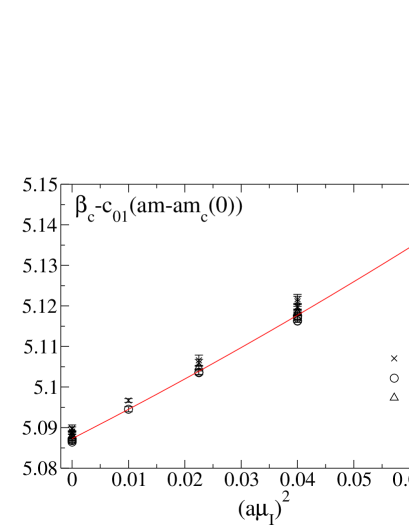
We conclude that we have a signal for a contribution to the critical coupling. This is a result of having more accurate data and does not invalidate our earlier observation that the line is well described by the leading term. E.g. at the contribution of this term to the critical coupling is only . Converting to continuum units by means of the two-loop beta-function as in [4], we thus obtain for the critical line in three flavor QCD
| (15) |
on the right side of this and the following two equations is meant to be the same as in the denominator on the left, which plays a role for the coefficient of next-to-leading terms. Note that the mixing of the errors on the parameters in the critical coupling through standard error propagation drowns out the -signal in continuum units. Since we do not yet have a signal for a mixed -term, the quark mass and chemical potential dependence are separately consistent with
| (16) |
A mixed dependence only appears in higher orders, having no effect at our present accuracy. This explains why critical lines obtained previously for various different quark masses agree so well [5].
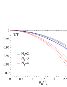
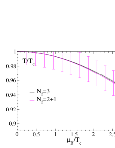
We may then directly compare our result with existing ones for [4] and [14] in Fig. 5. As one would expect, our result falls between these two. Note, however, that these earlier results were not sensitive to a -term, which makes itself felt at the right end of the interval and also lowers the -coefficient, cf. Table 1. Also shown in the figure is the result for as obtained by reweighting [2]. In accordance with our expectations from Sec. 3.1, due to the quark mass independence of the critical line this result is practically identical to the one for .
5.2 First order vs. crossover and error estimates
Before presenting our results for the cumulant ratio, we make some remarks concerning the considerable technical difficulty of these measurements. Inspection of the Monte Carlo history of an observable over a sufficiently long Monte Carlo time reveals that the tunneling frequency between the different vacua is very low: observing only one crossing per a few thousand trajectories is typical. This is expected in a first order regime, where tunneling is suppressed by a potential barrier, but the same observation is made in the crossover regime.
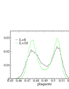
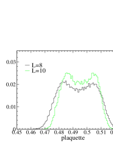
The reason for this behavior is the fact that, on the lattice sizes used here, the probability distributions for measurements at the critical coupling have not yet reached their asymptotic scaling regime. This is illustrated in Fig. 6, where we show the distributions of plaquette values on two volumes for a point each in the first order and crossover regimes. In accordance with expectation, the first order region displays a two peak structure and tunneling gets more suppressed on a larger volume. In the crossover region we observe accordingly a merging of the two peak structure with increasing volume. However, this merging to the asymptotic Gaussian distribution is not yet complete, and a remnant of the two-peak structure can be clearly identified. The displayed parameter values are deep in the crossover region, and the situation gets only worse closer to the critical point. This is a well known difficulty in the investigation of phase transitions.
On the other hand, the value of and its statistical error are driven by the number of tunnelings rather than the total number of measurements. Essentially the observable distinguishes between crossover and a first order transition by picking up the difference in the frequency of tunnelings. This leads to a much slower reduction of error bars than in the case of the critical couplings, where only the change of the observable between the two phases is needed, for which the number of measurements is relevant. Hence, too short Monte Carlo runs with less than a few tens of tunnelings tend to underestimate the statistical error on . More dangerous is the finite volume remnant of tunneling suppression in the crossover regime which can, for too short runs and combined with too small an error estimate, lead to an underestimate of and hence to misidentifying a crossover as a weakly first order signal.
In light of this, we can only be fully confident of our error estimates for lattices, where tunneling is faster and we have the longest Monte Carlo runs. On this volume we obtain a significant result for the -dependence, whereas for the signal is hidden in the noise. These volumes will be mainly used for consistency and scaling checks.
5.3 The cumulant ratio as function of and
Following Sec. 4, we proceed to discuss our measurements of the cumulant ratio along the critical line in order to determine its endpoint and its quark mass dependence. Our current accuracy constrains only the leading terms in the Taylor expansion of . To begin, we perform an analysis analogous to the one in [7]. For a fixed value of , we measure along the critical line , cf. Fig. 2 (right). The critical quark mass separating first order from crossover behavior is then extracted from the intersection of measured on different volumes. This is shown in Fig. 7 for and .
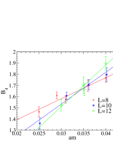
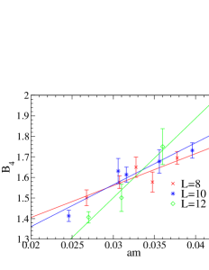
Our results for are in full agreement with those reported in [7], serving as a check of the analysis. The volume dependence appears to be moderate, and for the intersection point between the larger volumes we get , compared to [7]. However, practically the same result is obtained for , pointing to a very weak -dependence of . Indeed, plotting our data for fixed as a function of , no structure beyond noise is apparent to the eye.
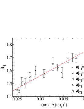
In order to obtain better accuracy we modify our analysis. Let us rewrite the leading terms of the Taylor expansion Eq. (11) as
| (17) |
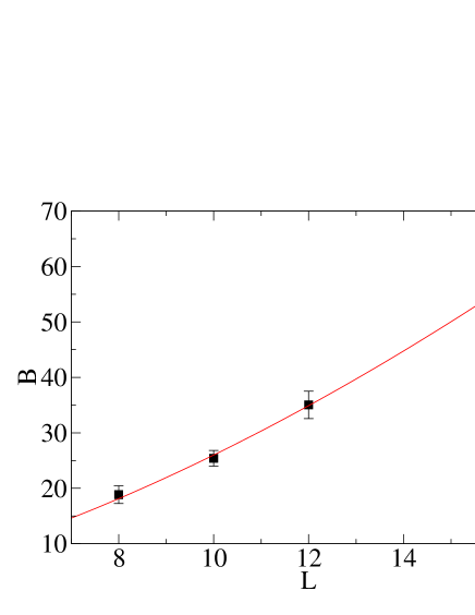
where we have traded the parameters for . With the constant fixed to its infinite volume value, finite volume corrections to will now show up in , which can be compared with the previous result. In this form we can collapse all our data obtained for various pairings into one plot and fit them by a single three parameter fit. Finally, , as in Eq. (13), is now immediately given by the fit parameter . Fig. 8 shows all data combined in this way together with the best fit. The fit results for all volumes are displayed in Table 2.
| 8 | 0. | 0313(5) | – | 18. | 5(1.8) | 1. | 33 | |
|---|---|---|---|---|---|---|---|---|
| 8 | 0. | 0323(6) | 0. | 044(19) | 18. | 9(1.6)) | 1. | 00 |
| 10 | 0. | 0325(3) | – | 25. | 9(1.3) | 0. | 54 | |
| 10 | 0. | 0320(5) | -0. | 010(10) | 25. | 4(2.1) | 0. | 53 |
| 12 | 0. | 0326(2) | – | 35. | 8(1.7) | 0. | 19 | |
| 12 | 0. | 0325(4) | -0. | 008(18) | 35. | 0(2.5) | 0. | 22 |
| 16 | 0. | 0331(3) | – | 57. | 0(6.3) | 0. | 19 | |
| 8-12 | 0. | 0323(3) | 0. | 0008(8) | 0. | 67(3) | 0. | 84 |
However, even after combining all data on one volume, the -coefficient is still only weakly constrained. The data on the larger lattices are consistent with a negligible -dependence, as is apparent by the acceptable fits obtained without such a term. Only on the lattice, for which we have the best statistics, do the fits prefer a positive value of this quantity.
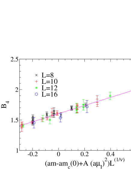
Let us now try to combine the different volumes by exploiting the fact that appears close to its infinite volume limit, and hence should be close to the scaling region on the volumes considered. In order to explicitly test for this, we plot the fit parameter against the volumes for which it was obtained, and fit the data to the expected asymptotic scaling behavior , cf. Eq. (14). For this purpose, we also use the data from [7]. This is shown in Fig. 9, and the resulting is indeed consistent with the Ising value . Having thus established the explicit volume dependence of as in Eq. (14), we may combine all available volumes into one maximally constrained fit, in order to get higher accuracy. This is done in Fig. 10. The resulting parameter values are given in the last line of Table 2.
5.4 The line of critical endpoints
The situation is less clear for the -dependence, as Table 2 shows. The combined fit over all volumes does not constrain the parameter enough to yield a non-vanishing result. Clearly, this is due to the lattices, whose results are consistent with zero, but whose negative central values neutralize the significant answer obtained on . Since these lattices only add noise to the determination of , we thus quote the number as our tentative final result,
| (18) |
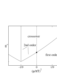
with higher terms being smaller than our present error of 40%. A check of the fit result is obtained by measuring for different quark masses along the vertical -line at , cf. Fig. 3, in order to determine . We have done so on and find , while Eq. (18) in lattice units predicts .
Note that, in terms of our natural expansion units, the coefficient of interest is not unnaturally small. Determining it to better accuracy is, however, a formidable numerical task that requires computational resources on the largest scales available. A more conservative result is obtained by adding two standard deviations to the central value, resulting in a bound at 90% confidence level.
Taken at face value, Eq. (18) tells us the critical bare quark mass for a given chemical potential as sketched in Fig. 3, while its inverse yields the location of the critical endpoint for a given bare quark mass. The renormalization of the bare quark mass cancels in the ratio, so that it should be independent of the lattice action chosen, up to additive cut-off effects. Moreover, since in the mass range of interest the zero temperature pion mass , we have
| (19) |
where MeV for unimproved (p4-improved (preliminary)) staggered fermions, respectively [7, 15]. These numbers highlight the strong need to eliminate cut-off effects on .
Another result involving only physical quantities is obtained by eliminating the bare quark mass in computing the line of critical endpoints,
| (20) |
While in this function we lose the information on the quark mass dependence, the curve relates only infrared quantities and describes a physical property of the QCD parameter space, cf. Fig. 2.
6 Discussion
Let us now try to compare our results to those obtained by other groups. The first Taylor coefficient in for the three flavor theory was also calculated by means of Taylor expanded reweighting [15]. In the form of Eq. (18) their result for the coefficient is , compared to ours of . We observe that, continued to imaginary , this result violates the bound derived in Sec. 3.1. The only way to avoid this conclusion would be large -effects, for which we see no evidence. While at present we have no explanation for this rather drastic disagreement, we speculate that it is a statistics problem: the preliminary result of [15] is based on six thousand trajectories, and measurements for different are always correlated in reweighting approaches. Considering the problems we mentioned in Sec. 5.2, the similarly sobering findings of Ref. [8], and the scatter of our uncorrelated data in Fig. 8, this might account for the discrepancy.
Eventually, we are of course interested in the 2+1 flavor theory with non-degenerate masses. In this case the line of constant derived from the leading order expression Eq. (11) reads
| (21) |
However, a linear extrapolation in the quark mass to is most likely not valid. Blindly substituting the bare quark masses of [2] and our value for , one would obtain a critical chemical potential GeV. While this number is certainly meaningless, it seems nevertheless that our calculation would put the critical endpoint of the deconfinement line at considerably larger values of than those reported in [2, 15]. To avoid extrapolations over large ranges, 2+1 flavor QCD with physical masses requires additional calculations in the light and heavier quark mass regimes and could be quite different numerically.
Finally we would like to add one more comment concerning the difficulties of distinguishing a first order phase transition from crossover, Sec. 5.2. Our discussion focused on the observable , and one may ask about its relevance for other methods of determining the endpoint, like finite size scaling of susceptibilities or Lee-Yang zeroes. While other observables might well have smaller statistical errors than when measured on the same number of configurations, their relative behavior between first order and crossover regimes is nevertheless driven by the number of tunnelings, and therefore suffers from the same slowness of the Monte Carlo history as our measurement, requiring similar statistics in order to arrive at reliable results.
7 Conclusions
We have investigated the finite density phase diagram of three flavor QCD for MeV by means of lattice simulations at imaginary chemical potential. Compared to previous studies with , we gathered much increased statistics allowing us to determine the location of the critical line through terms linear in the quark mass and quartic in the chemical potential. The curvature of the critical line becomes more negative with increasing . Any mixing terms between quark mass and chemical potential are smaller than our present accuracy, rendering quark mass independent to a good approximation.
We have also studied the nature of the phase transition along the critical line, and the location of its endpoint as a function of quark mass, by studying the Binder cumulant as a function of quark mass and chemical potential. We were able to compute the first coefficient of the critical quark mass to 40% accuracy. A constraint at the 90% confidence level puts our result at considerable odds with a preliminary result given by a Taylor expanded reweighting technique [15], our critical endpoint being at larger for comparable quark masses. Our central results are given in Eqs. (15),(16) and (18),(20). While we have clearly demonstrated the feasibility of such a calculation, our results exhibit the formidable difficulty of this task, whose unambiguous completion requires computational resources beyond those presently available to us. An extrapolation to the physical flavor case requires additional simulations to account for the heavier strange quark, and is envisaged for the future.
Acknowledgements
Our simulations were performed on main frame platforms as well as PC clusters at SCF Boston University, ETH Zürich, the University of Minnesota Supercomputer Institute, the RCNP at Osaka University, MIT and Jefferson Lab. We thank all those institutions for the provided resources, and in particular F. Berruto, A. Nakamura, J. Negele, A. Pochinsky and C. Rebbi for support in getting access to them. We are also grateful to N. Christ for providing us with Ref. [8] prior to publication, to C. Schmidt for correspondence and to M. Laine and K. Rajagopal for useful comments on the manuscript.
References
- [1] I. M. Barbour, S. E. Morrison, E. G. Klepfish, J. B. Kogut and M. P. Lombardo, Nucl. Phys. Proc. Suppl. 60A (1998) 220 [arXiv:hep-lat/9705042].
- [2] Z. Fodor and S. D. Katz, JHEP 0203 (2002) 014 [arXiv:hep-lat/0106002].
- [3] C. R. Allton et al., Phys. Rev. D 66 (2002) 074507 [arXiv:hep-lat/0204010].
- [4] P. de Forcrand and O. Philipsen, Nucl. Phys. B 642 (2002) 290 [arXiv:hep-lat/0205016].
- [5] E. Laermann and O. Philipsen, arXiv:hep-ph/0303042.
- [6] S. Aoki et al. [JLQCD Collaboration], Nucl. Phys. Proc. Suppl. 73 (1999) 459 [arXiv:hep-lat/9809102].
- [7] F. Karsch, E. Laermann and C. Schmidt, Phys. Lett. B 520 (2001) 41 [arXiv:hep-lat/0107020].
- [8] N. Christ and X. Liao, contribution to LATTICE 2002, to appear in the proceedings.
- [9] A. Roberge and N. Weiss, Nucl. Phys. B 275 (1986) 734.
- [10] M. P. Lombardo, Nucl. Phys. Proc. Suppl. 83 (2000) 375 [arXiv:hep-lat/9908006].
- [11] A. Hart, M. Laine and O. Philipsen, Phys. Lett. B 505 (2001) 141 [arXiv:hep-lat/0010008]; Nucl. Phys. B 586 (2000) 443 [arXiv:hep-ph/0004060].
- [12] P. de Forcrand and O. Philipsen, arXiv:hep-ph/0301209.
- [13] C. Schmidt, C. R. Allton, S. Ejiri, S. J. Hands, O. Kaczmarek, F. Karsch and E. Laermann, arXiv:hep-lat/0209009.
- [14] M. D’Elia and M. P. Lombardo, Phys. Rev. D 67 (2003) 014505 [arXiv:hep-lat/0209146].
- [15] C. R. Allton, S. Ejiri, S. J. Hands, O. Kaczmarek, F. Karsch, E. Laermann and C. Schmidt, arXiv:hep-lat/0305007.
- [16] K. Binder, Z. Phys. B 43 (1981) 119.
- [17] A. Vuorinen, arXiv:hep-ph/0305183.
- [18] S. Gottlieb, W. Liu, D. Toussaint, R. L. Renken and R. L. Sugar, Phys. Rev. D 35, 2531 (1987).
- [19] A. M. Ferrenberg and R. H. Swendsen, Phys. Rev. Lett. 63, 1195 (1989).