Effective lattice theories for Polyakov loops

Abstract:

We derive effective actions for $SU(2)$ Polyakov loops using inverse Monte Carlo techniques. In a first approach, we determine the effective couplings by requiring that the effective ensemble reproduces the single–site distribution of the Polyakov loops. The latter is flat below the critical temperature implying that the (untraced) Polyakov loop is distributed uniformly over its target space, the $SU(2)$ group manifold. This allows for an analytic determination of the Binder cumulant and the distribution of the mean–field, which turns out to be approximately Gaussian. In a second approach, we employ novel lattice Schwinger–Dyson equations which reflect the $SU(2)\times SU(2)$ invariance of the functional Haar measure. Expanding the effective action in terms of $SU(2)$ group characters makes the numerics sufficiently stable so that we are able to extract a total number of 14 couplings. The resulting action is short–ranged and reproduces the Yang–Mills correlators very well.

1 Introduction

The deconfinement phase transition in pure Yang–Mills theory [1, 2] is controlled by the dynamics of the Polyakov loop variable $\mathfrak{P}_{\mbox{\footnotesize\boldmath$x$}}$. Above a critical temperature $T_{c}$, the singlet part $L_{\mbox{\scriptsize\boldmath$x$}}\equiv\mbox{tr}\,\mathfrak{P}_{\mbox{\footnotesize\boldmath$x$}}/2$ develops a nonvanishing vacuum expectation value (VEV). In this high–temperature phase one expects to find a plasma of liberated gluons (and, in QCD, also quarks). The VEV of $L_{\mbox{\scriptsize\boldmath$x$}}$ thus represents an order parameter associated with spontaneous symmetry breaking. The symmetry in question is a global $\mathbb{Z}_{N}$ symmetry, $\mathbb{Z}_{N}$ being the center of the gauge group $SU(N)$. While the Yang–Mills action is center symmetric, $L_{\mbox{\scriptsize\boldmath$x$}}$, although gauge invariant, transforms nontrivially, $L_{\mbox{\scriptsize\boldmath$x$}}\to zL_{\mbox{\scriptsize\boldmath$x$}}$, $z\in\mathbb{Z}_{N}$. Combining renormalization group ideas and dimensional reduction, Svetitsky and Yaffe have conjectured that finite–temperature $SU(N)$ Yang–Mills theory in $d$ dimensions is in the universality class of a $\mathbb{Z}_{N}$ spin model in dimension $d-1$ [3, 4]. For some recent and rather sophisticated confirmations of the statement on the lattice the reader is referred to [5, 6, 7, 8].

The universality argument implies that effective field theory methods may be put to use. It should make sense to map the microscopic theory, here Yang–Mills, onto a macroscopic one, described by an effective action with $\mathbb{Z}_{N}$ symmetry. For gauge group $SU(2)$, for instance, one can try to coarse–grain the gauge fields all the way down to $\mathbb{Z}_{2}$ Ising spins [9, 10, 11]. An intermediate procedure is to establish an effective action for the Polyakov loop variable itself [12, 13, 14]. This may be achieved analytically using strong–coupling or, equivalently, high–temperature expansions [13, 15, 16]. Doing so for $SU(2)$, one obtains a local effective action depending on all characters $\chi_{j}(\mathfrak{P}_{\mbox{\footnotesize\boldmath$x$}})$ [15, 16]. The index $j\in\mathbb{N}/2$ labels the irreducible representations of $SU(2)$. In this most elementary case, $\chi_{j}$ can be expressed in terms of powers of $L_{\mbox{\scriptsize\boldmath$x$}}$ (the character of the fundamental representation, $j=1/2$). For larger gauge groups, however, more and more characters/representations become relevant. This fact has recently been employed for model building, regarding the untraced holonomy $\mathfrak{P}_{\mbox{\footnotesize\boldmath$x$}}$ [17] or, equivalently, its eigenvalues [18] as the fundamental degrees of freedom. We parametrize the (lattice) effective action as follows,

$$S_{\mathrm{eff}}=\sum_{a}\lambda_{a}S_{a}\;,$$ (1)

with center–symmetric operators $S_{a}$ and effective couplings $\lambda_{a}$ to be determined. As stated above, for $SU(2)$ it is sufficient to work with only the traced Polyakov loop, $L_{\mbox{\scriptsize\boldmath$x$}}$. The effective action will then have the form [14],

$$S_{\mathrm{eff}}[L_{\mbox{\scriptsize\boldmath$x$}}]=\sum_{\mbox{\scriptsize\boldmath$x$}}V[L_{\mbox{\scriptsize\boldmath$x$}}^{2}]+\sum_{\mbox{\scriptsize\boldmath$x$}\mbox{\scriptsize\boldmath$y$}}L_{\mbox{\scriptsize\boldmath$x$}}K_{\mbox{\scriptsize\boldmath$x$}\mbox{\scriptsize\boldmath$y$}}^{(2)}L_{\mbox{\scriptsize\boldmath$y$}}+\sum_{\mbox{\scriptsize\boldmath$x$}\mbox{\scriptsize\boldmath$y$}\mbox{\scriptsize\boldmath$u$}\mbox{\scriptsize\boldmath$v$}}L_{\mbox{\scriptsize\boldmath$x$}}L_{\mbox{\scriptsize\boldmath$y$}}K_{\mbox{\scriptsize\boldmath$x$}\mbox{\scriptsize\boldmath$y$}\mbox{\scriptsize\boldmath$u$}\mbox{\scriptsize\boldmath$v$}}^{(4)}L_{\mbox{\scriptsize\boldmath$u$}}L_{\mbox{\scriptsize\boldmath$v$}}+\ldots\;.$$ (2)

The kernels $K^{(a)}$ depend on the couplings $\lambda_{a}$ and the temperature. By construction, the $\mathbb{Z}_{2}$ center symmetry ($L_{\mbox{\scriptsize\boldmath$x$}}\to-L_{\mbox{\scriptsize\boldmath$x$}}$) is manifest. Note that the representation (2) is rather general and leaves room for a plethora of operators, the compact continuous variable $L_{\mbox{\scriptsize\boldmath$x$}}\in[-1,1]$ being dimensionless. Later on, it will therefore be crucial to choose an appropriate subset of all possible operators in order to capture the essential physics. In this respect it turns out useful to follow [17] and view the effective action (1) as being embedded into a ‘sigma model’ depending on $\mathfrak{P}_{\mbox{\footnotesize\boldmath$x$}}$, $S_{\mathrm{eff}}[L]\equiv S_{\mathrm{eff}}[\mathfrak{P}_{\mbox{\footnotesize\boldmath$x$}}]$. This yields an additional global $SU(2)$ symmetry,

$$\mathfrak{P}_{\mbox{\footnotesize\boldmath$x$}}\to g\,\mathfrak{P}_{\mbox{\footnotesize\boldmath$x$}}\,g^{-1}\;,\quad g\in SU(2)\;,$$ (3)

which is a remnant of the underlying $SU(2)$ gauge invariance. The Haar measure $\mathcal{D}\mathfrak{P}_{\mbox{\footnotesize\boldmath$x$}}$ has an even larger symmetry, namely $SU(2)\times SU(2)$, corresponding to the transformation law

$$\mathfrak{P}_{\mbox{\footnotesize\boldmath$x$}}\to g\,\mathfrak{P}_{\mbox{\footnotesize\boldmath$x$}}\,h\;,\quad g,h\in SU(2)\;.$$ (4)

The invariance of the measure leads to novel Schwinger–Dyson identities which will be an important ingredient in our derivation of the effective couplings $\lambda_{a}$ inherent in (1).

The paper is organized as follows. In Section 2 we derive exact (lattice) Schwinger–Dyson equations from the invariance of the Haar measure $\mathcal{D}\mathfrak{P}_{\mbox{\footnotesize\boldmath$x$}}$. We proceed by analysing the single–site distribution of the Polyakov loop variable $L_{\mbox{\scriptsize\boldmath$x$}}$ in Section 3. This yields a semianalytic method to determine all couplings $\lambda_{a}$ apart from the one of the hopping term, $\lambda_{0}$. The latter is obtained in Section 4 using the Schwinger–Dyson equations which are also employed to check the resulting effective action. In Section 5, we determine the effective potential in the symmetric phase from the single–site distribution. Finally, in Section 6, we perform an extensive numerical analysis to improve the effective action by including a maximum number of 14 operators. Some technicalities concerning the analysis of histograms are relegated to an appendix.

2 Haar measure and Schwinger–Dyson identities

The Polyakov loop variable on the lattice is given by a holonomy or parallel transport connecting the (periodic) boundaries in temporal direction,

$$\mathfrak{P}_{\mbox{\footnotesize\boldmath$x$}}\equiv\prod_{t=1}^{N_{t}}U_{t,\mbox{\scriptsize\boldmath$x$};0}\;,$$ (5)

where the $U$’s are the standard link variables on a lattice of size $N_{t}\times N_{s}^{3}$. The effective action for the Polyakov loops is obtained by inserting unity into the Yang–Mills partition function, such that (the trace of) (5) is imposed as a constraint,

$$Z_{\mathrm{YM}} = \int\mathcal{D}U\,\exp(-S_{W}[U])$$ (6)

$$= \int\mathcal{D}U\,\mathcal{D}\mathfrak{P}_{\mbox{\footnotesize\boldmath$$}}\,\delta\Big{(}\mbox{tr}\,\mathfrak{P}_{\mbox{\footnotesize\boldmath$x$}}-\mbox{tr}\prod_{t=1}^{N_{t}}U_{t,\mbox{\scriptsize\boldmath$x$};0}\Big{)}\,\exp(-S_{W}[U])$$

$$\equiv \int\mathcal{D}\mathfrak{P}_{\mbox{\footnotesize\boldmath$$}}\exp(-S_{\mathrm{eff}}[\mathfrak{P}_{\mbox{\footnotesize\boldmath$$}}])\;,$$

with $\mathcal{D}U$ and $\mathcal{D}\mathfrak{P}_{\mbox{\footnotesize\boldmath$$}}$ the appropriate Haar measures (see below) and $S_{W}$ the standard Wilson action. Of course, the integration over link variables $U$ in the last step cannot be performed exactly. For this reason one has to resort to effective actions as given by (1) and (2), for instance [3, 4, 14]. Using inverse Monte–Carlo (IMC) techniques, it should be possible to determine a reasonable effective action from Yang–Mills configurations.

The main ingredient for this procedure are the Schwinger–Dyson equations associated with the symmetry of the measure $\mathcal{D}\mathfrak{P}_{\mbox{\footnotesize\boldmath$$}}$ under (4). To derive those we choose the parametrization,

$$\mathfrak{P}_{\mbox{\footnotesize\boldmath$x$}}\equiv P_{\mbox{\scriptsize\boldmath$x$}}^{0}\,\Eins+i\tau^{a}P_{\mbox{\scriptsize\boldmath$x$}}^{a}\equiv P_{\mbox{\scriptsize\boldmath$x$}}^{\mu}\sigma^{\mu}\;,$$ (7)

which is in $SU(2)$, $\mathfrak{P}_{\mbox{\footnotesize\boldmath$x$}}^{\dagger}\mathfrak{P}_{\mbox{\footnotesize\boldmath$x$}}=\Eins$, if the components $P_{\mbox{\scriptsize\boldmath$x$}}^{\mu}$ define a three–sphere $S^{3}$ according to

$$P_{\mbox{\scriptsize\boldmath$x$}}^{\mu}P_{\mbox{\scriptsize\boldmath$x$}}^{\mu}=(P_{\mbox{\scriptsize\boldmath$x$}}^{0})^{2}+P_{\mbox{\scriptsize\boldmath$x$}}^{a}P_{\mbox{\scriptsize\boldmath$x$}}^{a}=1\;.$$ (8)

We mention in passing that the points $x$ where the Polyakov loop is given by center elements, $\mathfrak{P}_{\mbox{\footnotesize\boldmath$x$}}=\pm\Eins$, correspond to the positions of monopoles in the Polyakov gauge [19, 20, 21], a particular realization of ‘t Hooft’s Abelian projections [22].

In terms of the coordinates (7), the traced Polyakov loop becomes $L_{\mbox{\scriptsize\boldmath$x$}}=P_{\mbox{\scriptsize\boldmath$x$}}^{0}$, while the functional Haar measure can be written as

$$\mathcal{D}\mathfrak{P}_{\mbox{\footnotesize\boldmath$$}}\equiv\prod_{\mbox{\scriptsize\boldmath$x$}}d^{4}P_{\mbox{\scriptsize\boldmath$x$}}\;\delta(P_{\mbox{\scriptsize\boldmath$x$}}^{\mu}P_{\mbox{\scriptsize\boldmath$x$}}^{\mu}-1)\;.$$ (9)

Obviously, this is invariant under rotations $R\in SO(4)$ generated by the angular momenta

$$L_{\mbox{\scriptsize\boldmath$x$}}^{\mu\nu}\equiv-i\left(P_{\mbox{\scriptsize\boldmath$x$}}^{\mu}\frac{\partial}{\partial P_{\mbox{\scriptsize\boldmath$x$}}^{\nu}}-P_{\mbox{\scriptsize\boldmath$x$}}^{\nu}\frac{\partial}{\partial P_{\mbox{\scriptsize\boldmath$x$}}^{\mu}}\right)\;.$$ (10)

These can be split up into ‘electric’ and ‘magnetic’ components (or ‘boosts’ and 3$d$ ‘rotations’),

$$iL_{\mbox{\scriptsize\boldmath$x$}}^{0a} \equiv P_{\mbox{\scriptsize\boldmath$x$}}^{0}\frac{\partial}{\partial P_{\mbox{\scriptsize\boldmath$x$}}^{a}}-P_{\mbox{\scriptsize\boldmath$x$}}^{a}\frac{\partial}{\partial P_{\mbox{\scriptsize\boldmath$x$}}^{0}}\equiv iK_{\mbox{\scriptsize\boldmath$x$}}^{a}\;,$$ (11)

$$iL_{\mbox{\scriptsize\boldmath$x$}}^{ab} \equiv P_{\mbox{\scriptsize\boldmath$x$}}^{a}\frac{\partial}{\partial P_{\mbox{\scriptsize\boldmath$x$}}^{b}}-P_{\mbox{\scriptsize\boldmath$x$}}^{b}\frac{\partial}{\partial P_{\mbox{\scriptsize\boldmath$x$}}^{a}}\equiv i\epsilon^{abc}L_{\mbox{\scriptsize\boldmath$x$}}^{c}\;,\quad L_{\mbox{\scriptsize\boldmath$x$}}^{a}\equiv\frac{1}{2}\epsilon^{abc}L_{\mbox{\scriptsize\boldmath$x$}}^{bc}\;.$$ (12)

Summarizing, the $SO(4)$ generators $L_{\mbox{\scriptsize\boldmath$x$}}^{\mu\nu}$ rotate the four–vector $P_{\mbox{\scriptsize\boldmath$x$}}^{\mu}$, while the $SO(3)$ generators $L_{\mbox{\scriptsize\boldmath$x$}}^{a}$ rotate the three–vector $P_{\mbox{\scriptsize\boldmath$x$}}^{a}$. The self– and anti–selfdual combinations,

$$M_{\mbox{\scriptsize\boldmath$x$}}^{a}\equiv\frac{1}{2}(L_{\mbox{\scriptsize\boldmath$x$}}^{a}-K_{\mbox{\scriptsize\boldmath$x$}}^{a})\;,$$ (13)

$$N_{\mbox{\scriptsize\boldmath$x$}}^{a}\equiv\frac{1}{2}(L_{\mbox{\scriptsize\boldmath$x$}}^{a}+K_{\mbox{\scriptsize\boldmath$x$}}^{a})\;,$$ (14)

generate left and right multiplication, respectively,

$$\mathfrak{P}_{\mbox{\footnotesize\boldmath$x$}}\to g\,\mathfrak{P}_{\mbox{\footnotesize\boldmath$x$}}\;,\quad\mathfrak{P}_{\mbox{\footnotesize\boldmath$x$}}\to\mathfrak{P}_{\mbox{\footnotesize\boldmath$x$}}\,h\;,\quad g,h\in SU(2)\;.$$ (15)

Global $SU(2)$ (gauge) transformations of the Polyakov loop as given by (3) are generated by $L_{\mbox{\scriptsize\boldmath$x$}}^{ab}$ (or $L_{\mbox{\scriptsize\boldmath$x$}}^{a}$) which do not differentiate with respect to the trace $P_{\mbox{\scriptsize\boldmath$x$}}^{0}$ and thus leave any functional of $P_{\mbox{\scriptsize\boldmath$x$}}^{0}=L_{\mbox{\scriptsize\boldmath$x$}}$ invariant. Typical such invariants are

$$P_{\mbox{\scriptsize\boldmath$x$}}^{0}\;,\quad P_{\mbox{\scriptsize\boldmath$x$}}^{a}P_{\mbox{\scriptsize\boldmath$x$}}^{a}\equiv 1-P_{\mbox{\scriptsize\boldmath$x$}}^{0}P_{\mbox{\scriptsize\boldmath$x$}}^{0}\;,\ldots\;.$$ (16)

The Schwinger–Dyson equations that follow from the $SO(4)$ invariance of the Haar measure (9) are given by

$$\int\mathcal{D}\mathfrak{P}_{\mbox{\footnotesize\boldmath$$}}\,L_{\mbox{\scriptsize\boldmath$x$}}^{\mu\nu}\big{\{}F[\mathfrak{P}_{\mbox{\footnotesize\boldmath$$}}]\exp(-S_{\mathrm{eff}}[\mathfrak{P}_{\mbox{\footnotesize\boldmath$$}}])\big{\}}=0\;,$$ (17)

where $F[\mathfrak{P}_{\mbox{\footnotesize\boldmath$$}}]$ is an arbitrary functional of $\mathfrak{P}_{\mbox{\footnotesize\boldmath$x$}}$. As the effective action depends on $\mathfrak{P}_{\mbox{\footnotesize\boldmath$x$}}$ solely through the $SU(2)$ invariant $P_{\mbox{\scriptsize\boldmath$x$}}^{0}$, $S_{\mathrm{eff}}[\mathfrak{P}_{\mbox{\footnotesize\boldmath$$}}]\equiv S_{\mathrm{eff}}[P^{0}]$, only the generators $L_{\mbox{\scriptsize\boldmath$x$}}^{0a}\equiv K_{\mbox{\scriptsize\boldmath$x$}}^{a}$ lead to nontrivial relations which can be written as

$$\langle K_{\mbox{\scriptsize\boldmath$x$}}^{a}F[\mathfrak{P}_{\mbox{\footnotesize\boldmath$$}}]-F[\mathfrak{P}_{\mbox{\footnotesize\boldmath$$}}]K_{\mbox{\scriptsize\boldmath$x$}}^{a}S_{\mathrm{eff}}[\mathfrak{P}_{\mbox{\footnotesize\boldmath$$}}]\rangle=0\;,$$ (18)

using the expectation value notation,

$$\langle O\rangle\equiv Z^{-1}\int\mathcal{D}\mathfrak{P}_{\mbox{\footnotesize\boldmath$$}}\,O[\mathfrak{P}_{\mbox{\footnotesize\boldmath$$}}]\exp(-S_{\mathrm{eff}}[\mathfrak{P}_{\mbox{\footnotesize\boldmath$$}}])\;.$$ (19)

Because $K_{\mbox{\scriptsize\boldmath$x$}}^{a}$ transforms like a vector under gauge rotations, (18) in general will not be gauge invariant. However, we are still free to choose the functional $F[\mathfrak{P}_{\mbox{\footnotesize\boldmath$$}}]$ at our will. If we pick

$$F_{\mbox{\scriptsize\boldmath$x$}}^{a}[\mathfrak{P}_{\mbox{\footnotesize\boldmath$$}}]\equiv P_{\mbox{\scriptsize\boldmath$x$}}^{a}\,G[P^{0}]\;,$$ (20)

with an arbitrary functional $G[P^{0}]$, we have the action of $K_{\mbox{\scriptsize\boldmath$x$}}^{a}$,

$$K_{\mbox{\scriptsize\boldmath$x$}}^{a}F_{\mbox{\scriptsize\boldmath$y$}}^{b}=\delta^{ab}\delta_{\mbox{\scriptsize\boldmath$x$}\mbox{\scriptsize\boldmath$y$}}P_{\mbox{\scriptsize\boldmath$x$}}^{0}G-P_{\mbox{\scriptsize\boldmath$x$}}^{a}P_{\mbox{\scriptsize\boldmath$y$}}^{b}\,G_{\mbox{\scriptsize\boldmath$x$}}^{\prime}\;,$$ (21)

where we have denoted $G_{\mbox{\scriptsize\boldmath$x$}}^{\prime}\equiv\partial G/\partial P_{\mbox{\scriptsize\boldmath$x$}}^{0}$. Plugging this into (18), setting $\mbox{\boldmath$x$}=\mbox{\boldmath$y$}$ and taking the trace one finds the gauge invariant Schwinger–Dyson equations,

$$\langle 3P_{\mbox{\scriptsize\boldmath$x$}}^{0}G-P_{\mbox{\scriptsize\boldmath$x$}}^{a}P_{\mbox{\scriptsize\boldmath$x$}}^{a}(G_{\mbox{\scriptsize\boldmath$x$}}^{\prime}-GS_{\mathrm{eff},\mbox{\scriptsize\boldmath$x$}}^{\prime})\rangle=0\;.$$ (22)

The same result is obtained using $F_{\mbox{\scriptsize\boldmath$x$}}^{a}[\mathfrak{P}_{\mbox{\footnotesize\boldmath$$}}]\equiv K_{\mbox{\scriptsize\boldmath$x$}}^{a}\,H[P^{0}]$ instead of (20) and identifying $H_{\mbox{\scriptsize\boldmath$x$}}^{\prime}\equiv-G_{\mbox{\scriptsize\boldmath$x$}}$. Let us rewrite (22) as a functional integral,

$$\int\mathcal{D}\mathfrak{P}_{\mbox{\footnotesize\boldmath$$}}\,\left[3P_{\mbox{\scriptsize\boldmath$x$}}^{0}G-P_{\mbox{\scriptsize\boldmath$x$}}^{a}P_{\mbox{\scriptsize\boldmath$x$}}^{a}(G_{\mbox{\scriptsize\boldmath$x$}}^{\prime}-GS_{\mathrm{eff},\mbox{\scriptsize\boldmath$x$}}^{\prime})\right]\exp(-S_{\mathrm{eff}})=0\;,$$ (23)

and parametrize $\mathfrak{P}_{\mbox{\footnotesize\boldmath$x$}}$ according to

$$\mathfrak{P}_{\mbox{\footnotesize\boldmath$x$}}=\exp{i\tau^{a}\theta_{\mbox{\scriptsize\boldmath$x$}}^{a}}=\Eins\cos\theta_{\mbox{\scriptsize\boldmath$x$}}+i\tau^{a}n_{\mbox{\scriptsize\boldmath$x$}}^{a}\sin\theta_{\mbox{\scriptsize\boldmath$x$}}\;,\quad n_{\mbox{\scriptsize\boldmath$x$}}^{a}\equiv P_{\mbox{\scriptsize\boldmath$x$}}^{a}/(P_{\mbox{\scriptsize\boldmath$x$}}^{b}P_{\mbox{\scriptsize\boldmath$x$}}^{b})^{1/2}\;.$$ (24)

Then, the traced Polyakov loop is $L_{\mbox{\scriptsize\boldmath$x$}}\equiv\cos\theta_{\mbox{\scriptsize\boldmath$x$}}$ while the Haar measure (9) becomes

$$\mathcal{D}\mathfrak{P}_{\mbox{\footnotesize\boldmath$$}}=\prod_{\mbox{\scriptsize\boldmath$x$}}\sin^{2}\theta_{\mbox{\scriptsize\boldmath$x$}}\,\frac{d\theta_{\mbox{\scriptsize\boldmath$x$}}\,d^{2}n_{\mbox{\scriptsize\boldmath$x$}}}{4\pi^{2}}\;.$$ (25)

As the functional integral (23) only depends on invariants we can integrate over the directions $n$ (yielding an irrelevant volume factor) so that we are left with an integral involving only the reduced Haar measure,

$$\mathcal{D}L\equiv\prod_{\mbox{\scriptsize\boldmath$x$}}d\theta_{\mbox{\scriptsize\boldmath$x$}}\,\sin^{2}\theta_{\mbox{\scriptsize\boldmath$x$}}=\prod_{\mbox{\scriptsize\boldmath$x$}}d(\cos\theta_{\mbox{\scriptsize\boldmath$x$}})\sin\theta_{\mbox{\scriptsize\boldmath$x$}}=\prod_{\mbox{\scriptsize\boldmath$x$}}dL_{\mbox{\scriptsize\boldmath$x$}}\,\sqrt{1-L_{\mbox{\scriptsize\boldmath$x$}}^{2}}\equiv\prod_{\mbox{\scriptsize\boldmath$x$}}DL_{\mbox{\scriptsize\boldmath$x$}}\;,$$ (26)

namely,

$$\int\prod_{\mbox{\scriptsize\boldmath$y$}}d\theta_{\mbox{\scriptsize\boldmath$y$}}\,\sin^{2}\theta_{\mbox{\scriptsize\boldmath$y$}}\left[3\cos\theta_{\mbox{\scriptsize\boldmath$x$}}G-\sin^{2}\theta_{\mbox{\scriptsize\boldmath$x$}}(G_{\mbox{\scriptsize\boldmath$x$}}^{\prime}-GS_{\mathrm{eff},\mbox{\scriptsize\boldmath$x$}}^{\prime})\right]\exp(-S_{\mathrm{eff}})=0\;.$$ (27)

A more compact form for these relations is achieved in terms of total derivatives,

$$0 = \int\prod_{\mbox{\scriptsize\boldmath$y$}\neq\mbox{\scriptsize\boldmath$x$}}d\theta_{\mbox{\scriptsize\boldmath$y$}}\sin^{2}\theta_{\mbox{\scriptsize\boldmath$y$}}\int d\theta_{\mbox{\scriptsize\boldmath$x$}}\,\frac{\delta}{\delta\theta_{\mbox{\scriptsize\boldmath$x$}}}\left\{\sin^{3}\theta_{\mbox{\scriptsize\boldmath$x$}}\,G\,\exp(-S_{\mathrm{eff}})\right\}$$ (28)

$$= \int\prod_{\mbox{\scriptsize\boldmath$y$}\neq\mbox{\scriptsize\boldmath$x$}}d\theta_{\mbox{\scriptsize\boldmath$y$}}\sin^{2}\theta_{\mbox{\scriptsize\boldmath$y$}}\int d(\cos\theta_{\mbox{\scriptsize\boldmath$x$}})\,\frac{\delta}{\delta(\cos\theta_{\mbox{\scriptsize\boldmath$x$}})}\left\{\sin^{3}\theta_{\mbox{\scriptsize\boldmath$x$}}\,G\,\exp(-S_{\mathrm{eff}})\right\}\;.$$

Note that the $\sin^{3}\theta$ term ensures the absence of surface terms. With (28) we have found the Schwinger–Dyson relations of the reduced theory involving only the invariant $L=\cos\theta$. We do not have a simple geometrical explanation for the invariance of the reduced Haar measure $\mathcal{D}L$ leading to (28). The $SO(4)$ symmetry of the measure $\mathcal{D}\mathfrak{P}_{\mbox{\footnotesize\boldmath$$}}$, however, is very natural.

In terms of the Polyakov loop $L_{\mbox{\scriptsize\boldmath$x$}}$, (27) is the expectation value

$$\langle 3L_{\mbox{\scriptsize\boldmath$x$}}G-(1-L_{\mbox{\scriptsize\boldmath$x$}}^{2})(G_{\mbox{\scriptsize\boldmath$x$}}^{\prime}-GS_{\mathrm{eff},\mbox{\scriptsize\boldmath$x$}}^{\prime})\rangle=0\;.$$ (29)

Comparing with (22) we notice that it does not matter whether the expectation value is taken with the full or reduced Haar measure as long as $G=G[L]$. If we insert the ansatz (1), the Schwinger–Dyson equations (29) become a linear system for the couplings $\lambda_{a}$,

$$\sum_{a}\langle(1-L_{\mbox{\scriptsize\boldmath$x$}}^{2})\,GS_{a,\mbox{\scriptsize\boldmath$x$}}^{\prime}\rangle\,\lambda_{a}=\langle(1-L_{\mbox{\scriptsize\boldmath$x$}}^{2})\,G_{\mbox{\scriptsize\boldmath$x$}}^{\prime}\rangle-3\,\langle L_{\mbox{\scriptsize\boldmath$x$}}G\rangle\;.$$ (30)

To solve this unambiguously we need as many independent operators $G$ as there are couplings $\lambda_{a}$. A particularly natural procedure, which also turns out to be rather stable numerically, is to choose $G\equiv S_{b,\mbox{\scriptsize\boldmath$y$}}^{\prime}$. Any of these operators contains an odd number of $L_{\mbox{\scriptsize\boldmath$x$}}$’s so that the minimal set of Schwinger–Dyson equations relates only nontrivial expectation values,

$$\sum_{a}\langle(1-L_{\mbox{\scriptsize\boldmath$x$}}^{2})\,S_{b,\mbox{\scriptsize\boldmath$y$}}^{\prime}S_{a,\mbox{\scriptsize\boldmath$x$}}^{\prime}\rangle\,\lambda_{a}=\langle(1-L_{\mbox{\scriptsize\boldmath$x$}}^{2})\,S_{b,\mbox{\scriptsize\boldmath$y$}\mbox{\scriptsize\boldmath$x$}}^{\prime\prime}\rangle-3\,\langle L_{\mbox{\scriptsize\boldmath$x$}}S_{b,\mbox{\scriptsize\boldmath$y$}}^{\prime}\rangle\;.$$ (31)

At this stage, keeping $x$ and $y$ fixed, the problem of determining the couplings $\lambda_{a}$ is well posed mathematically. Numerically, of course, it is better to use all the information one can get, for instance by scanning through all possible distances $x\equiv|\mbox{\boldmath$x$}-\mbox{\boldmath$y$}|$, $x<N_{s}/2$. The resulting overdetermined system is then solved by least–square methods. Another possibility is to add new equations to (31) by choosing further appropriate monomials or polynomials in $L_{\mbox{\scriptsize\boldmath$x$}}$ for the operator $G$. This philosophy will be extensively adopted in Section 6. Before that, however, we will try to proceed in a (semi–)analytical fashion.

3 Single–site distributions of Polyakov loops

3.1 Definitions

From the effective action of Polyakov loops $S_{\mathrm{eff}}[L]$ one can derive new probability densities by integrating over (part of) the loop variables $L$. Of course, this amounts to some kind of course–graining so that via the new densities one will only have access to gross properties of the effective action. Nevertheless, these densities, if chosen properly, exactly reproduce certain expectation values calculated within the full effective ensemble. Consider, for instance, the local moments,

$$\ell_{p}\equiv\langle L_{\mbox{\scriptsize\boldmath$x$}}^{p}\rangle\equiv Z^{-1}\int\prod_{\mbox{\scriptsize\boldmath$y$}}DL_{\mbox{\scriptsize\boldmath$y$}}\,L_{\mbox{\scriptsize\boldmath$x$}}^{p}\exp\left(-S_{\mathrm{eff}}[L]\right)\;,$$ (32)

where, as usual, the partition function $Z$ is the integral over $\exp(-S_{\mathrm{eff}})$. Splitting off the $L_{\mbox{\scriptsize\boldmath$x$}}$–integration, (32) can be rewritten as

$$\ell_{p}=\langle L_{\mbox{\scriptsize\boldmath$x$}}^{p}\rangle\equiv\int_{-1}^{1}DL_{\mbox{\scriptsize\boldmath$x$}}\,L_{\mbox{\scriptsize\boldmath$x$}}^{p}\,p_{W}[L_{\mbox{\scriptsize\boldmath$x$}}]\equiv\langle L_{\mbox{\scriptsize\boldmath$x$}}^{p}\rangle_{W}\;,$$ (33)

with the probability density $p_{W}$ obtained via integrating over all $L_{\mbox{\scriptsize\boldmath$y$}}\neq L_{\mbox{\scriptsize\boldmath$x$}}$,

$$p_{W}[L_{\mbox{\scriptsize\boldmath$x$}}]\equiv Z^{-1}\int\prod_{\mbox{\scriptsize\boldmath$y$}\neq\mbox{\scriptsize\boldmath$x$}}DL_{\mbox{\scriptsize\boldmath$y$}}\,\exp\left(-S_{\mathrm{eff}}[L_{\mbox{\scriptsize\boldmath$y$}}]\right)\equiv Z^{-1}\exp\left(-W[L_{\mbox{\scriptsize\boldmath$x$}}]\right)\;.$$ (34)

Due to translational invariance, $p_{W}$ (like $\ell_{p}$) does not depend on the site $x$. Thus, $DL\,p_{W}[L]$ is the probability to find the value of the Polyakov loop in the interval $[L,L+dL]$. The $\mathbb{Z}_{2}$–symmetry of the effective action implies that the power $p$ in (32) and (33) has to be even, $p=2q$, at least for finite volume (no spontaneous symmetry breaking). Therefore, knowing $p_{W}$ gives access to all local moments $\ell_{2q}$ and (by taking the logarithm) to all local cumulants $c_{2q}$ as well. A particularly important quantity is the Binder cumulant [23, 24], defined as the quotient

$$b_{4}\equiv\frac{c_{4}}{c_{2}^{2}}=\frac{\ell_{4}}{\ell_{2}^{2}}-3\;,$$ (35)

which measures the deviation from a Gaussian distribution. This will be analysed in some detail later on.

From the definition (34) it is obvious that $p_{W}$ is blind against spatial correlations of Polyakov loops. In other words, one cannot calculate two–point functions like $G_{\mbox{\scriptsize\boldmath$x$}\mbox{\scriptsize\boldmath$y$}}\equiv\langle L_{\mbox{\scriptsize\boldmath$x$}}L_{\mbox{\scriptsize\boldmath$y$}}\rangle$. In principle, this can be remedied by a slight generalization of (34). To this end we define a new probability density depending on $L_{\mbox{\scriptsize\boldmath$x$}}$ and $L_{\mbox{\scriptsize\boldmath$y$}}$,

$$p_{W_{2}}[L_{\mbox{\scriptsize\boldmath$x$}},L_{\mbox{\scriptsize\boldmath$y$}}]\equiv Z^{-1}\int\prod_{\mbox{\scriptsize\boldmath$z$}\neq\mbox{\scriptsize\boldmath$x$},\mbox{\scriptsize\boldmath$y$}}DL_{\mbox{\scriptsize\boldmath$z$}}\,\exp\left(-S_{\mathrm{eff}}[L]\right)\equiv Z^{-1}\exp\left(-W_{2}[L_{\mbox{\scriptsize\boldmath$x$}},L_{\mbox{\scriptsize\boldmath$y$}}]\right)\;.$$ (36)

Then, one can calculate the following two–point correlators,

$$\langle L_{\mbox{\scriptsize\boldmath$x$}}^{p}L_{\mbox{\scriptsize\boldmath$y$}}^{q}\rangle=\int DL_{\mbox{\scriptsize\boldmath$x$}}\,DL_{\mbox{\scriptsize\boldmath$y$}}\,L_{\mbox{\scriptsize\boldmath$x$}}^{p}L_{\mbox{\scriptsize\boldmath$y$}}^{q}\,p_{W_{2}}[L_{\mbox{\scriptsize\boldmath$x$}},L_{\mbox{\scriptsize\boldmath$y$}}]\;.$$ (37)

Obviously, $p_{W}$ and $p_{W_{2}}$ are related according to

$$p_{W}[L_{\mbox{\scriptsize\boldmath$x$}}]=\int DL_{\mbox{\scriptsize\boldmath$y$}}\,p_{W_{2}}[L_{\mbox{\scriptsize\boldmath$x$}},L_{\mbox{\scriptsize\boldmath$y$}}]\;.$$ (38)

If there were no correlations, one would have factorization, $p_{W_{2}}[L_{\mbox{\scriptsize\boldmath$x$}},L_{\mbox{\scriptsize\boldmath$y$}}]=p_{W}[L_{\mbox{\scriptsize\boldmath$x$}}]p_{W}[L_{\mbox{\scriptsize\boldmath$y$}}]$.

3.2 Determination of single–site distributions

At first glance, there seems to be not much of a gain by introducing densities like the single–site distribution $p_{W}$. Note, however, that $p_{W}[L]$ is much simpler than our original density $p_{S}\equiv Z^{-1}\exp(-S_{\mathrm{eff}})$ which depends on $N_{s}^{3}$ variables rather than just one. In addition, $p_{W}$ can be obtained rather easily from our Monte Carlo data. The results are fairly smooth histograms which are displayed in Figure 1 (for details see App. A). The most important observation, however, is the finding that $p_{W}$ is flat below $T_{c}$, that is, one has an equipartition for $L_{\mbox{\scriptsize\boldmath$x$}}$. Apparently, this is a remnant of the $SO(4)$ symmetry discussed in Section 2. Taking the (negative) logarithm of $p_{W}$ we obtain the single–site potential $W[L]$ shown in Figure 2.

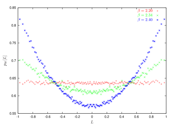
Figure 1: Single–site density $p_{W}[L]$ for temperatures above ($\times$,$*$) and below $T_{c}$ ($+$). For $T<T_{c}$ ($\beta<\beta_{c}\simeq 2.299$), the density is flat, $p_{W}=2/\pi$. Input: 200 to 400 configurations, $N_{s}=20$.

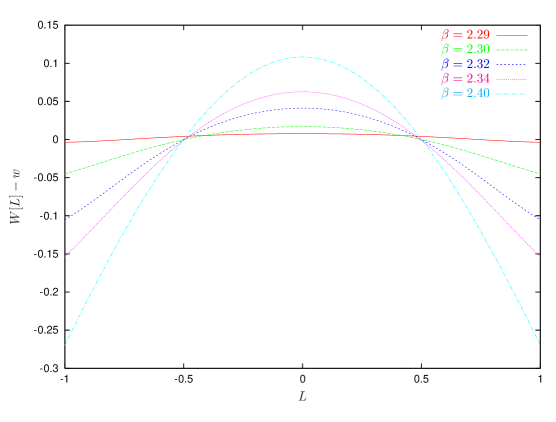
Figure 2: The single–site potential $W[L]$ shifted by the constant offset $w$. For $T<T_{c}$ ($\beta<\beta_{c}\simeq 2.299$), $W[L]$ is flat. Input: 200 to 400 configurations, $N_{s}=20$.

We are thus led to employ the following ansatz for the potential $W$ from (34), distinguishing between temperatures below ($-$) and above ($+$) the critical value, $T_{c}$,

$$W_{-}[L] = const\;,$$ (39)

$$W_{+}[L] = const^{\prime}+\sum_{k}\frac{\kappa_{2k}}{2k}L_{\mbox{\scriptsize\boldmath$x$}}^{2k}\;.$$ (40)

Demanding $\langle 1\rangle=1$ these imply for the density $p_{W}$,

$$p_{W}^{-}[L] = \exp(-W_{-})/Z_{-}=2/\pi\;,$$ (41)

$$p_{W}^{+}[L] = \exp(-W_{+}[L])/Z_{+}\;.$$ (42)

Things are particularly straightforward below $T_{c}$, so let us discuss this case first. The result (41) shows that, after normalization, the single–site distribution of Polyakov loops below $T_{c}$ is known exactly. Furthermore, it is simple enough so that the associated (local) moments can be determined analytically,

$$\ell_{2q}^{-}\equiv\langle L^{2q}\rangle_{W_{-}}=\frac{2}{\pi}\int_{-1}^{1}dL\,\sqrt{1-L^{2}}\,L^{2q}=\frac{1}{\sqrt{\pi}}\frac{\Gamma(q+1/2)}{\Gamma(q+2)}=2^{-q}\,\frac{(2q-1)!!}{(q+1)!}\;.$$ (43)

The generating function for these moments can also be calculated explicitly,

$$Z_{-}(t)\equiv\langle e^{tL}\rangle_{W_{-}}=\frac{2}{\pi}\int DL\,e^{tL}=\sum_{l\geq 0}\frac{\ell_{2l}^{-}}{(2l)!}t^{2l}=\frac{2}{t}\,I_{1}(t)\;,$$ (44)

$I_{1}$ being the standard modified Bessel function. For the Binder cumulant (35) we thus find the result

$$b_{4}^{-}=\frac{\ell_{4}^{-}}{(\ell_{2}^{-})^{2}}-3=\frac{1/8}{(1/4)^{2}}-3=-1\;.$$ (45)

We have checked that (43) and (45) hold numerically both for the histograms $p_{W}$ and the effective Yang–Mills probability density $p_{S}$. The results for the Binder cumulant are displayed in Figure 3.

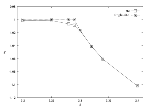
Figure 3: The Binder cumulant $b_{4}$ as obtained from the simulated Yang–Mills configurations ($\Box$) with $N_{s}=20$ compared to the single–site distribution $p_{W}$ ($*$). Below $\beta_{c}\simeq 2.30$, the exact result (41) for $p_{W}$ (i.e. $W=const$) has been used. Above $\beta_{c}$, $W$ has been fitted to a polynomial (see below).

It may seem strange that we get a flat distribution $p_{W}$ below $T_{c}$. However, this does not imply that the effective potential, which defines the distribution of the mean field $\bar{L}$, becomes trivial (see Sect. 5).

To proceed, we have to specify our ansatz for the effective action beyond (1) and (2). Svetitsky and Yaffe have argued [3, 4, 14] that, close to the phase transition, the effective interactions should be short ranged so that $S_{\mathrm{eff}}$ is of Ginzburg–Landau type,

$$S_{\mathrm{eff}}=\lambda_{0}\sum_{\mbox{\scriptsize\boldmath$x$},\mbox{\scriptsize\boldmath$i$}}L_{\mbox{\scriptsize\boldmath$x$}}L_{\mbox{\scriptsize\boldmath$x$}+\mbox{\scriptsize\boldmath$i$}}+\sum_{\mbox{\scriptsize\boldmath$x$}}\sum_{k>0}\frac{\lambda_{2k}}{2k}(L_{\mbox{\scriptsize\boldmath$x$}})^{2k}\equiv\lambda_{0}S_{0}+\lambda_{2}S_{2}+\ldots\;.$$ (46)

The high–temperature character expansions mentioned in the introduction yield additional hopping terms of the form $L_{\mbox{\scriptsize\boldmath$x$}}^{p}L_{\mbox{\scriptsize\boldmath$y$}}^{q}\ldots$ [15, 16, 25]. The relevance of these terms will be dicussed in Section 6.

Let us investigate the consequences of the ansatz (46) for the single–site distribution. Plugging the former into the definition (34) yields

$$e^{-W_{-}} = \int_{-1}^{1}\prod_{\mbox{\scriptsize\boldmath$y$}\neq\mbox{\scriptsize\boldmath$x$}}DL_{\mbox{\scriptsize\boldmath$y$}}\,\exp\left(-\lambda_{0}\sum_{\mbox{\scriptsize\boldmath$y$},i}L_{\mbox{\scriptsize\boldmath$y$}}L_{\mbox{\scriptsize\boldmath$y$}+\mbox{\scriptsize\boldmath$i$}}-\sum_{\mbox{\scriptsize\boldmath$y$},k>0}\frac{\lambda_{2k}}{2k}L_{\mbox{\scriptsize\boldmath$y$}}^{2k}\right)$$ (47)

$$= \exp\left(-\sum_{k>0}\frac{\lambda_{2k}}{2k}L_{\mbox{\scriptsize\boldmath$x$}}^{2k}\right)\!\int_{-1}^{1}\prod_{\mbox{\scriptsize\boldmath$y$}\neq\mbox{\scriptsize\boldmath$x$}}DL_{\mbox{\scriptsize\boldmath$y$}}\,\exp\left(-\lambda_{0}L_{\mbox{\scriptsize\boldmath$x$}}M_{\mbox{\scriptsize\boldmath$x$}}\right)\exp(-S^{\prime}_{\mathrm{eff}}[L_{\mbox{\scriptsize\boldmath$y$}}])\;,$$

where, in the second line, we have introduced the field

$$M_{\mbox{\scriptsize\boldmath$x$}}\equiv\frac{\partial S_{0}}{\partial L_{\mbox{\scriptsize\boldmath$x$}}}=\sum_{i}(L_{\mbox{\scriptsize\boldmath$x$}+\mbox{\scriptsize\boldmath$i$}}+L_{\mbox{\scriptsize\boldmath$x$}-\mbox{\scriptsize\boldmath$i$}})\;,$$ (48)

representing the sum of all nearest neighbors of $L_{\mbox{\scriptsize\boldmath$x$}}$. In addition, we have defined a modified action $S^{\prime}_{\mathrm{eff}}$ which is obtained from $S_{\mathrm{eff}}$ by setting $L_{\mbox{\scriptsize\boldmath$x$}}=0$,

$$S^{\prime}_{\mathrm{eff}}[L]\equiv S_{\mathrm{eff}}[L]\big{|}_{L_{\mbox{\scriptsize\boldmath$x$}}=0}\;.$$ (49)

Now, the left–hand side of (47) is $2Z_{-}/\pi$ and hence independent of $L_{\mbox{\scriptsize\boldmath$x$}}$. Thus we may put $L_{\mbox{\scriptsize\boldmath$x$}}=0$ everywhere on the right–hand side yielding the identity,

$$2Z_{-}/\pi=e^{-W_{-}}=\int_{-1}^{1}\prod_{\mbox{\scriptsize\boldmath$y$}\neq\mbox{\scriptsize\boldmath$x$}}DL_{\mbox{\scriptsize\boldmath$y$}}\,\exp(-S^{\prime}_{\mathrm{eff}}[L_{\mbox{\scriptsize\boldmath$y$}}])\equiv Z^{\prime}\;.$$ (50)

Accordingly, $e^{-W_{-}}$ is the partition function associated with action $S^{\prime}_{\mathrm{eff}}$. We can go one step further and expand the exponential containing the nearest–neighbor field $M_{\mbox{\scriptsize\boldmath$x$}}$ on the right–hand side of (47). This is actually a hopping–parameter expansion in $\lambda_{0}$ which, upon using (50), implies

$$1=\exp\left(-\sum_{k>0}\frac{\lambda_{2k}}{2k}L_{\mbox{\scriptsize\boldmath$x$}}^{2k}\right)\sum_{n\geq 0}\frac{(-\lambda_{0})^{n}}{n!}L_{\mbox{\scriptsize\boldmath$x$}}^{n}\langle M_{\mbox{\scriptsize\boldmath$x$}}^{n}\rangle^{\prime}\;.$$ (51)

Here, we have defined modified expectation values associated with $S^{\prime}_{\mathrm{eff}}$ and $Z^{\prime}$,

$$\langle O[L]\rangle^{\prime}\equiv\int\prod_{\mbox{\scriptsize\boldmath$y$}\neq\mbox{\scriptsize\boldmath$x$}}DL_{\mbox{\scriptsize\boldmath$y$}}\,O[L]\,\exp(-S^{\prime}_{\mathrm{eff}}[L])/Z^{\prime}\;.$$ (52)

The $\mathbb{Z}_{2}$–symmetry of the effective action requires $n$ to be even, $n=2m$. Denoting

$$\mu_{2m}\equiv\langle M_{\mbox{\scriptsize\boldmath$x$}}^{2m}\rangle^{\prime}\;,$$ (53)

we finally have

$$\sum_{m=0}^{\infty}\frac{\lambda_{0}^{2m}\mu_{2m}}{(2m)!}\,L_{\mbox{\scriptsize\boldmath$x$}}^{2m}=\exp\left(\sum_{k=1}^{\infty}\frac{\lambda_{2k}}{2k}L_{\mbox{\scriptsize\boldmath$x$}}^{2k}\right)\;.$$ (54)

To lowest order in $L_{\mbox{\scriptsize\boldmath$x$}}$ ($m=0$) this consistently reproduces the normalization (50), $\langle 1\rangle^{\prime}=1=e^{-W_{-}}/Z^{\prime}$. A general interpretation can be given as follows. To have equipartition requires a delicate balance between the hopping term ($\lambda_{0}$) and the ‘potential’ terms ($\lambda_{2k}$). Setting $\lambda_{0}=0$ (so that the effective action leads to a product measure) implies that all $\lambda_{2k}$ have to vanish and vice versa: $\lambda_{2k}=0$ implies $\lambda_{0}=0$.

To further evaluate the identity (54) we note that it can be viewed as a particular example of a linked–cluster or Mayer expansion [26, 27, 28] expressing the moments $\lambda_{0}^{2m}\mu_{2m}$ in terms of the cumulants

$$\lambda_{2k}^{\prime}\equiv(2k-1)!\;\lambda_{2k}\;.$$ (55)

The relation between moments and cumulants can actually be solved for arbitrary $m$ (see e.g. [29]),

$$\lambda_{0}^{2m}\mu_{2m}=\sum_{n=1}^{m}\frac{1}{n!}\sum_{k_{1},\ldots,k_{n}=1\atop k_{1}+\ldots+k_{n}=m}^{m}\frac{(2m)!}{(2k_{1})!\ldots(2k_{n})!}\prod_{i=1}^{n}\lambda_{2k_{i}}^{\prime}\;.$$ (56)

This somewhat clumsy formula yields for the first few orders

$$\lambda_{0}^{2}\,\mu_{2} = \lambda_{2}^{\prime}\;,$$ (57)

$$\lambda_{0}^{4}\,\mu_{4} = \lambda_{4}^{\prime}+3\,\lambda_{2}^{\prime 2}\;,$$ (58)

$$\lambda_{0}^{6}\,\mu_{6} = \lambda_{6}^{\prime}+15\,\lambda_{2}^{\prime}\lambda_{4}^{\prime}+15\,\lambda_{2}^{\prime 3}\;,$$ (59)

$$\lambda_{0}^{8}\,\mu_{8} = \lambda_{8}^{\prime}+28\,\lambda_{2}^{\prime}\lambda_{6}^{\prime}+35\,\lambda_{4}^{\prime 2}+210\,\lambda_{4}^{\prime}\lambda_{2}^{\prime 2}+105\,\lambda_{2}^{\prime 4}\;.$$ (60)

It is quite obvious that by inverting (56) we can express the couplings $\lambda_{2k}$ (or cumulants $\lambda_{2k}^{\prime}$) in terms of the moments $\mu_{2m}$. Alternatively, one may take the logarithm of (54) and compare coefficients. In any case, the first few cumulants are

$$\lambda_{2}^{\prime} = \lambda_{0}^{2}\,\mu_{2}\;,$$ (61)

$$\lambda_{4}^{\prime} = \lambda_{0}^{4}\left(\mu_{4}-3\,\mu_{2}^{2}\right)\;,$$ (62)

$$\lambda_{6}^{\prime} = \lambda_{0}^{6}\left(\mu_{6}-15\,\mu_{4}\mu_{2}+30\,\mu_{2}^{3}\right)\;,$$ (63)

$$\lambda_{8}^{\prime} = \lambda_{0}^{8}\left(\mu_{8}-28\,\mu_{6}\mu_{2}+420\,\mu_{4}\mu_{2}^{2}-630\,\mu_{2}^{4}-35\mu_{4}^{2}\right)\;.$$ (64)

These identities almost solve our problem of determining $S_{\mathrm{eff}}$ as they express the unknown couplings $\lambda_{2k}$ in terms of $\lambda_{0}$ (unknown as yet) and the modified expectation values $\mu_{2m}$ from (53).

Things become simple if one allows for only a finite number (say $K$) of couplings $\lambda_{2k}$ in the Svetitsky–Yaffe action (46). Then, there is only a finite number of independent moments $\mu_{2k}$, $k=1,\ldots K$. This is quite obvious from e.g. (64). Setting $\lambda_{8}=0=\lambda_{8}^{\prime}$ determines the moment $\mu_{8}$ and all higher ones in terms of $\mu_{2}$, $\mu_{4}$ and $\mu_{6}$.

For $K=1$, (54) yields the general expression

$$\mu_{2m}=(2m-1)!!\,\left(\frac{\lambda_{2}}{\lambda_{0}^{2}}\right)^{m}\equiv(2m-1)!!\;\mu_{2}^{m}\;,\quad m=1,2,\ldots\;.$$ (65)

We thus have found factorization: all higher moments $\mu_{2m}$, $m>1$ can be expressed in terms of the lowest one, $\mu_{2}\equiv\lambda_{2}/\lambda_{0}^{2}$. Of course, this is consistent with $S_{\mathrm{eff}}$ being quadratic in $L_{\mbox{\scriptsize\boldmath$x$}}$ (vanishing of quartic and higher cumulants $\lambda_{2k}^{\prime}$).

For $K=2$, we have three couplings, $\lambda_{0}$, $\lambda_{2}$ and $\lambda_{4}$. In this case, (54) implies the following generalization of (65),

$$\mu_{2m}=(2m-1)!!\;\mu_{2}^{m}\sum_{k=0}^{[m/2]}{m\choose 2k}(2k-1)!!\left(\frac{\mu_{4}}{3\mu_{2}^{2}}-1\right)^{k}\;,$$ (66)

which shows that all moments $\mu_{2m}$ can be expressed in terms of $\mu_{2}$ and $\mu_{4}$. The first two factors in the sum count the number of ways in which one can form $k$ pairs out of $m$ elements. The term raised to power $k$ is actually (one third of) the Binder cumulant associated with the moments $\mu_{2m}$. If it were zero we would get back at (65).

Clearly, in order to determine the couplings $\lambda_{2k}$ one does not want to calculate the moments $\mu_{2k}$ by performing a new and costly Monte Carlo simulation with the action $S^{\prime}_{\mathrm{eff}}$, setting $L_{\mbox{\scriptsize\boldmath$x$}}=0$ at a particular site $x$. One expects, however, that, for large lattices, one will have the approximate identity

$$\langle M^{2m}\rangle^{\prime}\simeq\langle M^{2m}\rangle\;,\quad m>0\;,$$ (67)

where the latter expectation is taken in the full Yang–Mills ensemble. For our numerical evaluation we have tested assumption (67) as follows. Define the expectation values

$$\langle M_{\mbox{\scriptsize\boldmath$x$}}^{2m}\rangle_{\Lambda}\equiv Z_{\Lambda}^{-1}\int\prod_{\mbox{\scriptsize\boldmath$y$}}DL_{\mbox{\scriptsize\boldmath$y$}}\,M_{\mbox{\scriptsize\boldmath$x$}}^{2m}\exp\big{(}-S_{\mathrm{eff}}[L_{\mbox{\scriptsize\boldmath$y$}}]-\Lambda L_{\mbox{\scriptsize\boldmath$x$}}^{2}\big{)}\;,$$ (68)

so that one has

$$\langle M_{\mbox{\scriptsize\boldmath$x$}}^{2m}\rangle=\langle M_{\mbox{\scriptsize\boldmath$x$}}^{2m}\rangle_{0}\;,\quad\langle M_{\mbox{\scriptsize\boldmath$x$}}^{2m}\rangle^{\prime}=\langle M_{\mbox{\scriptsize\boldmath$x$}}^{2m}\rangle_{\infty}\;.$$ (69)

If (67) is to hold then $\langle M_{\mbox{\scriptsize\boldmath$x$}}^{2m}\rangle_{\Lambda}$ must be approximately independent of $\Lambda$. We have checked this by simulating the leading–order action,

$$S_{\Lambda}\equiv\frac{\lambda_{0}}{2}\sum_{\langle\mbox{\scriptsize\boldmath$x$}\mbox{\scriptsize\boldmath$y$}\rangle}L_{\mbox{\scriptsize\boldmath$x$}}L_{\mbox{\scriptsize\boldmath$y$}}+\Lambda L_{\mbox{\scriptsize\boldmath$x$}}^{2}\equiv\lambda_{0}\sum_{\mbox{\scriptsize\boldmath$x$},\mbox{\scriptsize\boldmath$i$}}L_{\mbox{\scriptsize\boldmath$x$}}L_{\mbox{\scriptsize\boldmath$x$}+\mbox{\scriptsize\boldmath$i$}}+\Lambda L_{\mbox{\scriptsize\boldmath$x$}}^{2}\;,$$ (70)

for different values of $\Lambda$ on a lattice of size $16^{3}$ with $\lambda_{0}=-0.3$ (symmetric phase). The calculated expectation values $\langle M_{\mbox{\scriptsize\boldmath$x$}}^{2}\rangle_{\Lambda}$ displayed in Table 1 show that $\langle M_{\mbox{\scriptsize\boldmath$x$}}^{2}\rangle_{\Lambda}$ is indeed independent of $\Lambda$ to an accuracy of about 0.5 %.

$\Lambda$	0	1	10	100	1000	10000
$\langle M_{\mbox{\scriptsize\boldmath$x$}}^{2}\rangle_{\Lambda}$	1.951	1.947	1.962	1.954	1.939	1.961

Table 1: The expectation value $\langle M_{\mbox{\scriptsize\boldmath$x$}}^{2}\rangle_{\Lambda}$ as a function of the parameter $\Lambda$ suppressing the single–site variable $L_{\mbox{\scriptsize\boldmath$x$}}$. Input parameters are $N_{s}=16$, $\lambda_{0}=-0.3$ (symmetric phase).

For $T>T_{c}$, we use the ansatz (40). This implies that formulae (51–64) still hold, however, with $\lambda_{2k}$ now replaced by $\lambda_{2k}-\kappa_{2k}$. We have checked that the identification (67) also holds in the broken phase (choosing $\lambda_{0}=-1$, see Table 2).

$\Lambda$	0	1	10	100	1000	10000
$\langle M_{\mbox{\scriptsize\boldmath$x$}}^{2}\rangle_{\Lambda}$	18.79	18.87	18.83	18.78	18.80	18.78

Table 2: The expectation value $\langle M_{\mbox{\scriptsize\boldmath$x$}}^{2}\rangle_{\Lambda}$ as a function of the parameter $\Lambda$ suppressing the single–site variable $L_{\mbox{\scriptsize\boldmath$x$}}$. Input parameters are $N_{s}=16$, $\lambda_{0}=-1$ (broken phase).

The couplings $\kappa_{2k}$ can be obtained by fitting $W_{+}[L]$ (see Figure 2) according to (40). The fit values are displayed in Tables 3 and 4.

$\beta$	$\kappa_{2}/2$	$\kappa_{4}/4$
2.40	$-0.4468$	0.0703
2.34	$-0.2712$	0.0526
2.32	$-0.1772$	0.0261
2.30	$-0.0717$	0.0120

Table 3: Two–parameter fit to $W_{+}[L]$.

$\beta$	$\kappa_{2}/2$	$\kappa_{4}/4$	$\kappa_{6}/6$
2.40	$-0.4531$	0.0901	$-0.0152$
2.34	$-0.2626$	0.0249	0.0216
2.32	$-0.1612$	$-0.0259$	0.0408
2.30	$-0.0666$	$-0.0087$	0.0133

Table 4: Three–parameter fit to $W_{+}[L]$.

Summarizing we note that we have good analytical and numerical control of the single–site distribution $p_{W}$ or, equivalently, the histograms displayed in Figure 1. Below $T_{c}$, the histogram is flat, $p_{W}^{-}=const$, above $T_{c}$, $W^{+}\sim\log p_{W}^{+}$ is a simple polynomial in $L^{2}$ with coefficients given in Tables 3 and 4.

4 Determination of the effective action

The calculation of the couplings $\lambda_{2k}$, $k\geq 0$, in the effective action proceeds in three steps. First we determine the moments $\mu_{2m}$ from the Polyakov–loop ensemble using the approximate identity (67). Second, from (61–64), we obtain the couplings $\lambda_{2k}=\lambda^{\prime}_{2k}/(2k-1)!$, $k>0$, in terms of the moments $\mu_{2k}$ and $\lambda_{0}$. Third, we determine $\lambda_{0}$.

The first step consists of straightforward numerics based on our Wilson ensembles obtained for several values of $\beta$ near $\beta_{c}$. The results for the $\mu_{2m}$ are displayed in Table 5.

$\beta$	2.20	2.25	2.28	2.29	2.30	2.32	2.34	2.40
$\mu_{2}$	1.93	2.086	2.242	2.327	2.466	2.946	3.336	4.173
$\mu_{4}$	10.16	11.55	13.07	13.89	15.27	20.16	24.22	33.60
$\mu_{6}$	80.88	96.06	113.0	121.7	137.6	194.1	241.5	357.6
$\mu_{8}$	829.3	1019	1237	1341	1551	2297	2922	4536

Table 5: The moments $\mu_{2m}$ for different values of the Wilson coupling $\beta$ ($N_{s}=20$).

With the moments $\mu_{2m}$ at hand we find the couplings

$$\lambda_{2k}=\lambda_{0}^{2k}\alpha_{2k}\;,\quad k>0\;,$$ (71)

where the $\alpha_{2k}$ can be expressed in terms of the $\mu_{2k}$ according to (61–64). The final step consists in the determination of $\lambda_{0}$. To this end we make use of the Schwinger–Dyson relations (30) choosing the operators $G\equiv L_{\mbox{\scriptsize\boldmath$x$}}^{2l-1}$ which results in

$$\langle(1-L_{\mbox{\scriptsize\boldmath$x$}}^{2})\,M_{\mbox{\scriptsize\boldmath$x$}}L_{\mbox{\scriptsize\boldmath$x$}}^{2l-1}\rangle\lambda_{0}+\sum_{k>0}\langle(1-L_{\mbox{\scriptsize\boldmath$x$}}^{2})\,L_{\mbox{\scriptsize\boldmath$x$}}^{2k+2l-2}\rangle\lambda_{2k}=(2l-1)\,\langle(1-L_{\mbox{\scriptsize\boldmath$x$}}^{2})\,L_{\mbox{\scriptsize\boldmath$x$}}^{2l-2}\rangle-3\,\langle L_{\mbox{\scriptsize\boldmath$x$}}^{2l}\rangle.$$ (72)

For $T<T_{c}$, where the single–site distribution is known exactly, the right–hand side of (72) vanishes. This can either be inferred from the analytical result (43) or by noting that the term in question is a total derivative,

$$(2l-1)\,\langle(1-L_{\mbox{\scriptsize\boldmath$x$}}^{2})\,L_{\mbox{\scriptsize\boldmath$x$}}^{2l-2}\rangle-3\,\langle L_{\mbox{\scriptsize\boldmath$x$}}^{2l}\rangle=-\frac{2}{\pi}\int_{-1}^{1}dL\,\frac{\partial}{\partial L}\left[(1-L^{2})^{3/2}\,L^{2l-1}\right]=0\;.$$ (73)

Plugging (71) into (72) and dividing by $\lambda_{0}$ (assumed to be nonzero) yields a nonlinear equation of degree $2k-1$ in $\lambda_{0}$. With the coefficients $\alpha_{2k}$ and all nonlocal expectation values (correlators) determined numerically, the coupling $\lambda_{0}$ can be obtained straightforwardly. As there are $2k-1$ solutions we take the one which is approximately independent of the number $K$ of couplings $\lambda_{2k}$. The resulting values of all couplings (for $K=2$ and $K=3$) are displayed in Tables 6 and 7.

$\beta$	2.20	2.25	2.28	2.29	2.30	2.32	2.34	2.40
$\lambda_{0}$	$-0.438$	$-0.473$	$-0.500$	$-0.509$	$-0.630$	$-0.685$	$-0.697$	$-0.725$
$\lambda_{2}/2$	0.186	0.233	0.280	0.301	0.453	0.603	0.675	0.873
$\lambda_{4}/4$	$-0.002$	$-0.003$	$-0.005$	$-0.007$	$-0.019$	$-0.053$	$-0.088$	$-0.212$

Table 6: Numerical values for the couplings $\lambda_{0}$ and $\lambda_{2k}/2k$, $k\leq K=2$. The critical Wilson coupling is $\beta_{c}=2.299$ ($N_{s}=20$).

$\beta$	2.20	2.25	2.28	2.29	2.30	2.32	2.34	2.40
$\lambda_{0}$	$-0.438$	$-0.476$	$-0.507$	$-0.510$	$-0.628$	$-0.690$	$-0.705$	$-0.760$
$\lambda_{2}/2$	0.186	0.237	0.288	0.303	0.453	0.621	0.698	0.979
$\lambda_{4}/4$	$-0.002$	$-0.003$	$-0.006$	$-0.007$	$-0.020$	$-0.057$	$-0.093$	$-0.256$
$\lambda_{6}/6$	0.000039	0.00011	0.00027	0.00037	0.0020	0.0106	0.0244	0.116

Table 7: Numerical values for the couplings $\lambda_{0}$ and $\lambda_{2k}/2k$, $k\leq K=3$. The critical Wilson coupling is $\beta_{c}=2.299$ ($N_{s}=20$).

With the effective couplings determined we are in the position to check our results by simulating the effective action. For both $\beta=2.20$ and $\beta=2.40$ we have produced 10000 configurations distributed according to $S_{\mathrm{eff}}$ using the couplings from Table 7.

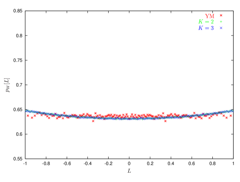
Figure 4: Comparison of single–site histograms based on simulating Yang–Mills ($*$) vs. the effective action for $T<T_{c}$. The curves for two and three couplings $\lambda_{2k}$, i.e. $K=2$ ($+$) and $K=3$ ($\times$), respectively, fall on top of each other. Input: $\beta=2.20$, $N_{s}=20$.

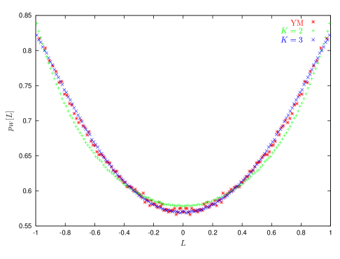
Figure 5: Comparison of single–site histograms based on simulating Yang–Mills ($*$) vs. the effective action with two ($+$) and three ($\times$) couplings $\lambda_{2k}$ for $T>T_{c}$. Input: $\beta=2.40$, $N_{s}=20$.

In Figures 4 and 5 we compare the single–site distributions obtained from the effective theory with those of Yang–Mills. The outcome is quite satisfactory. In particular, one notes that the inclusion of a $L^{6}$–term ($K=3$) still improves the matching of the histograms compared to the case $K=2$.

A further important check is provided by reproducing the input couplings of Table 7 via our IMC procedure. The results displayed in Table 8 show quite convincingly that the method works. If we allow for additional operators in the numerics (which are not present in the effective action) the numbers of Table 8 remain unchanged while the couplings of the new operators are consistently of order $10^{-5}$, i.e. compatible with zero.

$\beta$		$\lambda_{0}$	$\lambda_{2}$	$\lambda_{4}$	$\lambda_{6}$
2.20	input	$-0.43803$	$0.37182$	$-0.00681$	$0.00024$
2.20	output	$-0.43824$	$0.37351$	$-0.00621$	$0.00020$
2.40	input	$-0.76000$	$1.9572$	$-1.0216$	$0.69761$
2.40	output	$-0.76027$	$1.9605$	$-1.0222$	$0.69039$

Table 8: Comparison of couplings used as input of simulation with couplings obtained as output of IMC applied to the effective action.

5 The constraint effective potential

With an effective action being found, one could go on and calculate the constraint effective potential [30] which defines the distribution of the constant mean field,

$$\bar{L}\equiv\frac{1}{\Omega}\sum_{\mbox{\scriptsize\boldmath$x$}}L_{\mbox{\scriptsize\boldmath$x$}}\;,\quad\Omega=N_{s}^{3}\;.$$ (74)

In perturbation theory, the effective potential has been evaluated long ago [31, 32]. It describes a ‘gas’ of gluons at high temperature, i.e. deep in the deconfined phase. Recent models for the effective potential which also describe the confined phase are based on the eigenvalues of the Polyakov loop $\mathfrak{P}_{\mbox{\footnotesize\boldmath$x$}}$ [18] and not just their sum $L_{\mbox{\scriptsize\boldmath$x$}}$. As stated in the introduction, this difference becomes obsolete for $SU(2)$.

It thus seems of interest to investigate the effective potential on the lattice. This apparently requires further Monte–Carlo simulations of the effective action $S_{\mathrm{eff}}[L]$ with the mean field $\bar{L}$ held fixed, following the approach adopted in [30, 33]. It turns out, however, that these additional efforts can be avoided by making use of some statistical properties of the single–site distribution $p_{W}$ discussed in Section 3.

The constraint effective potential $V$ is defined in terms of the probability density of the mean field (74),

$$p_{V}[\bar{L}]\equiv Z_{V}^{-1}e^{-\Omega V[\bar{L}]}\equiv Z^{-1}\int\mathcal{D}L\,\delta\Big{(}\bar{L}-\Omega^{-1}\sum_{\mbox{\scriptsize\boldmath$x$}}L_{\mbox{\scriptsize\boldmath$x$}}\Big{)}\exp(-S_{\mathrm{eff}}[L])\;,$$ (75)

with the normalization $Z_{V}$ given by the partition function

$$Z_{V}\equiv Z_{V}(0)\equiv\int_{-1}^{1}d\bar{L}\,e^{-\Omega V[\bar{L}]}\;.$$ (76)

In what follows, we will try to obtain the mean–field distribution $p_{V}$ from the single–site distribution $p_{W}$. We note, first of all, that, due to translational invariance, the first moments coincide,

$$\langle\bar{L}\rangle_{V}\equiv\int d\bar{L}\,\bar{L}\,p_{V}[\bar{L}]=\Omega^{-1}\sum_{\mbox{\scriptsize\boldmath$x$}}Z^{-1}\int\prod_{\mbox{\scriptsize\boldmath$y$}}DL_{\mbox{\scriptsize\boldmath$y$}}\,L_{\mbox{\scriptsize\boldmath$x$}}\,e^{-S_{\mathrm{eff}}[L]}\equiv\langle L\rangle_{W}\equiv\langle L\rangle\;.$$ (77)

The higher moments, on the other hand, are different,

$$\langle L^{p}\rangle_{W} = \int\prod_{\mbox{\scriptsize\boldmath$y$}}DL_{\mbox{\scriptsize\boldmath$y$}}\,L_{\mbox{\scriptsize\boldmath$x$}}^{p}\,e^{-S_{\mathrm{eff}}[L]}=\langle L^{p}\rangle$$ (78)

$$\langle\bar{L}^{p}\rangle_{V} = \Omega^{-p}\sum_{\mbox{\scriptsize\boldmath$x$}_{1},\ldots\mbox{\scriptsize\boldmath$x$}_{p}}\langle L_{\mbox{\scriptsize\boldmath$x$}_{1}}\ldots L_{\mbox{\scriptsize\boldmath$x$}_{p}}\rangle\equiv\chi^{(p)}\;.$$ (79)

For the mean–field distribution we thus get generalized susceptibilities $\chi^{(p)}$, while $p_{W}$ yields expectation values of arbitrary powers of $L$ at a single spatial site, taken in the ensemble of Polyakov loops extracted from Yang–Mills. This has been discussed at length in Section 3.

To obtain a connection between arbitrary moments we suppose that the generating functions associated with $p_{V}$ and $p_{W}$ are related according to

$$Z_{V}(t)\equiv\langle\exp{t\bar{L}}\rangle_{V}=\langle\prod_{\mbox{\scriptsize\boldmath$x$}}\exp(tL_{\mbox{\scriptsize\boldmath$x$}}/\Omega)\rangle_{V}\stackrel{{\scriptstyle!}}{{\simeq}}\prod_{\mbox{\scriptsize\boldmath$x$}}\langle\exp(tL/\Omega)\rangle_{W}\equiv[Z_{W}(t/\Omega)]^{\Omega}\;.$$ (80)

Here, we have made the assumption that only a small fraction of the random variables $\{L_{\mbox{\scriptsize\boldmath$x$}}:\mbox{\boldmath$x$}\in\Omega\}$ are statistically dependent. This is justified for large volumes and short–range correlations. According to the law of large numbers we expect the collective random variable $\bar{L}=\sum_{\mbox{\scriptsize\boldmath$x$}}L_{\mbox{\scriptsize\boldmath$x$}}/\Omega$ to have a Gaussian distribution if the $L_{\mbox{\scriptsize\boldmath$x$}}$ are randomly distributed. Let us check to which extent this is realized.

Below $T_{c}$, $Z_{W}\equiv Z_{-}$ is exactly known from (44) so that

$$Z_{V}(t)\simeq\left[\frac{2\Omega}{t}I_{1}(t/\Omega)\right]^{\Omega}=\sum_{k}\frac{t^{2k}}{(2k)!}\langle\bar{L}^{2k}\rangle\;,\quad Z_{V}(0)=1\;.$$ (81)

Thus, by expanding the Bessel function (to power $\Omega$) we know all moments or susceptibilities of $p_{V}$. Explicitly, one finds

$$\langle\bar{L}^{2}\rangle_{V} = \frac{1}{4\Omega}\;,$$ (82)

$$\langle\bar{L}^{4}\rangle_{V} = \frac{1}{8\Omega^{3}}+\frac{3(\Omega-1)}{16\Omega^{3}}\;,$$ (83)

$$\langle\bar{L}^{6}\rangle_{V} = \frac{5}{64\Omega^{5}}+\frac{15(\Omega-1)}{32\Omega^{5}}+\frac{15(\Omega-1)(\Omega-2)}{64\Omega^{5}}\;.$$ (84)

In the large–volume limit, $\Omega\to\infty$, the leading terms yield

$$\langle\bar{L}^{2k}\rangle_{V}=\frac{(2k-1)!!}{(4\Omega)^{k}}=(2k-1)!!\,\langle\bar{L}^{2}\rangle_{V}^{k}\;,$$ (85)

an identity typical for a Gaussian distribution. As a cross check, we calculate the Binder cumulant associated with $p_{V}$. From (82) and (83) we have

$$b_{4,V}\equiv\frac{\langle\bar{L}^{4}\rangle_{V}}{\langle\bar{L}^{2}\rangle_{V}^{2}}-3=-\frac{1}{\Omega}\;,$$ (86)

which obviously vanishes in the infinite–volume limit in accordance with (85). Summing up the moments (85), we obtain the large–volume partition function

$$Z_{V}(t)\simeq\exp(t^{2}/8\Omega)\;,$$ (87)

which turns out to be Gaussian in $t$. Substituting $t=iu$, we have

$$Z_{V}(iu)=\int d\bar{L}\,\exp(-\Omega V[\bar{L}]+iu\bar{L})\simeq\exp(-u^{2}/8\Omega)\;.$$ (88)

To extract the mean–field distribution $p_{V}=\exp(-\Omega V)/Z_{V}$ we take the Fourier transform with respect to $u$ and find

$$p_{V}[\bar{L}]\simeq\sqrt{2\Omega/\pi}\,\exp(-2\Omega\bar{L}^{2})\;,$$ (89)

which is a perfect Gaussian distribution with variance

$$\sigma^{2}\equiv 1/4\Omega=\langle\bar{L}^{2}\rangle_{V}\;.$$ (90)

The fact that $\bar{L}$ is compact does not really matter as in the large–volume limit assumed, the Gaussian is sharply localized at $\bar{L}=0$. This is indeed seen from Figure 6 which shows that a Gaussian fit to the distribution of $\bar{L}$,

$$p_{V,\mathrm{fit}}[\bar{L}]=\frac{1}{\sqrt{2\pi}\sigma}\,\exp(-\bar{L}^{2}/2\sigma^{2})\;,$$ (91)

works perfectly well.

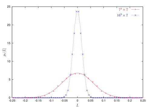
Figure 6: Gaussian fits to the distribution $p_{V}[\bar{L}]$ obtained from simulating Yang–Mills on lattices of size $16^{3}\times 7$ and $7^{3}\times 7$. The value $N_{t}=7$ for the temporal extension corresponds to the symmetric phase.

This is corroborated by comparing the fit values for $\sigma$ with the expectation values calculated from Yang–Mills as displayed in Table 9 for different volumes and bin sizes.

$\Omega\times N_{t}$	config.s/bin	$\sigma$	$\langle\bar{L}^{2}\rangle^{1/2}$
$7^{3}\times 6$	120	0.0837	0.0773
$7^{3}\times 6$	80	0.0845	0.0773
$7^{3}\times 7$	120	0.0582	0.0549
$7^{3}\times 7$	80	0.0588	0.0549
$16^{3}\times 6$	250	0.0249	0.0252
$16^{3}\times 7$	150	0.0167	0.0164
$16^{3}\times 7$	250	0.0167	0.0164

Table 9: Width $\sigma$ of the Gaussian fit (91) compared to the expectation value $\langle\bar{L}^{2}\rangle^{1/2}$ calculated from the $SU(2)$ Monte Carlo ensemble. The values for the temporal extension $N_{t}$ correspond to the symmetric phase.

The agreement between the fitted width and the expectation value $\langle\bar{L}^{2}\rangle^{1/2}$ is quite impressive, in particular for large volumes, as expected. Due to the approximations made, however, we do not reproduce the absolute numbers given by (90). If we define

$$\gamma\equiv\frac{\sigma^{2}(\Omega_{1})}{\sigma^{2}(\Omega_{2})}=\frac{\Omega_{2}}{\Omega_{1}}\;,$$ (92)

we get for $\Omega_{1}=7^{3}$ and $\Omega_{2}=16^{3}$ the numerical value $\gamma=(16/7)^{3}=11.94$ while the results of Table 9 yield

$$\gamma = 11.1\pm 0.4\;,\quad N_{t}=6\;,$$ (93)

$$\gamma = 11.5\pm 0.9\;,\quad N_{t}=7\;,$$ (94)

where the error has been estimated by varying the bin sizes. Thus, at least for sufficiently low temperature (large $N_{t}$) we obtain the correct scaling of the width with the volume.

6 Reproducing the two–point function

The procedure developed so far is based on the single–site distribution of the Polyakov loop which is under good (semianalytic) control. By construction, the effective action obtained in this way reproduces the Yang–Mills distribution quite well (recall Fig.s 4 and 5). At this point it is natural to ask how well we are reproducing correlators of the Polyakov loop. After all, these are intimately related to the confining potential ($T<T_{c}$) or the Debye mass ($T>T_{c}$), see e.g. [14]. In Fig.s 7 and 8 we compare the Yang–Mills two–point function with the one obtained from the Svetitsky–Yaffe effective action (46) using the couplings from Table 8.

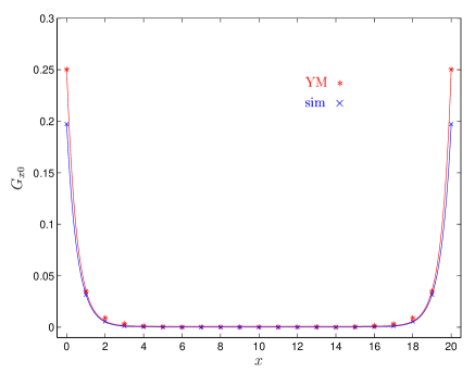
Figure 7: The Yang–Mills two–point function (YM) compared to the one obtained from the Svetitsky–Yaffe effective action with four couplings (sim). Input: $\beta=2.20$, $N_{s}=20$.

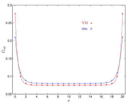
Figure 8: The Yang–Mills two–point function (YM) compared to the one obtained from the Svetitsky–Yaffe effective action with four couplings (sim). Input: $\beta=2.40$, $N_{s}=20$.

The figures suggest that we are doing quite well in the symmetric phase ($\beta=2.20$, i.e. $T<T_{c}$). In the broken phase ($\beta=2.40$, i.e. $T>T_{c}$), however, there is room for improvement both in the exponential decay and the value $\langle L\rangle^{2}$ of the plateau. To assess the (dis)agreement quantitatively, we fit all two–point functions according to

$$G_{x0}\equiv\langle L_{\mbox{\scriptsize\boldmath$x$}}L_{\mbox{\scriptsize\boldmath$0$}}\rangle=a\big{[}\exp(-bx)+\exp\big{(}-b(N_{s}-x)\big{)}\big{]}+c\;.$$ (95)

The values for the fit parameters are listed in Table 10 and corroborate the qualitative statements made above.

$\beta$		$a$	$b$	$c$
2.20	YM	$0.2493$	$1.9627$	$0.0009$
	sim	$0.1971$	$1.8309$	$0.0001$
2.40	YM	$0.2006$	$2.0715$	$0.0752$
	sim	$0.1295$	$1.4499$	$0.0802$

Table 10: Comparison of the fit parameters from (95) associated with Fig.s 7 and 8.

In order to improve the matching between the effective theory and Yang–Mills we obviously have to include more operators. In previous applications of IMC, this has mainly been done for Ising systems [10, 11, 34, 35] or twodimensional nonlinear sigma models [36, 37]. In these cases, the set of operators is restricted as they square to unity. For the Polyakov loop, however, the situation is different, as arbitrary (ultralocal) powers as well as hopping terms associated with arbitrary powers are allowed, i.e. terms like $L_{\mbox{\scriptsize\boldmath$x$}_{1}}^{p_{1}}L_{\mbox{\scriptsize\boldmath$x$}_{2}}^{p_{2}}L_{\mbox{\scriptsize\boldmath$x$}_{3}}^{p_{3}}\ldots$. It turns out the the IMC procedure tends to get destabilized upon including more and more monomials in $L_{\mbox{\scriptsize\boldmath$x$}}$. As a result, the values for the couplings depend rather strongly on the number of operators present and of equations used in the overdetermined linear system. In addition, the determinants of the matrices to be inverted may become as small as $10^{-40}$. We thus had to work with symbolic programs like Maple, setting the number of digits to 60 or even more. Nevertheless, the instabilities prevailed. Inspired by the results from the high–temperature expansion on the lattice [15, 16], we have tried to overcome these problems by changing our operator basis from monomials in $L$ to characters. Being orthogonal class functions, these seem to be the natural candidates for an economic set of operators. At this point it should be noted that for an effective action with a finite number of terms different choices of bases are not equivalent.

As stated in the introduction, for $SU(2)$ the characters can be expressed as polynomials in the traced Polyakov loop, $L=\mbox{tr}\mathfrak{P}_{\mbox{\footnotesize\boldmath$$}}/2=\cos\theta$, according to

$$\chi_{j}(L)\equiv\frac{\sin\big{(}(2j+1)\theta\big{)}}{\sin\theta}=\sum_{p=0}^{[j]}(-1)^{p}{2j+1\choose 2p+1}L^{2j-2p}(1-L^{2})^{p}\;,\quad j=0,{\textstyle\frac{1}{2}},1,\ldots\;.$$ (96)

This formula allows to reobtain the $L$–representation from the characters. The first few relations are

$$\chi_{1/2}=2L\;,\quad\chi_{1}=4L^{2}-1\;,\quad\chi_{3/2}=8L^{3}-4L\;,\quad\ldots\;.$$ (97)

These are sufficient to obtain monomials up to terms of order $L_{\mbox{\scriptsize\boldmath$x$}}^{3}L_{\mbox{\scriptsize\boldmath$y$}}^{3}$. To streamline notation it is useful to define a basic link variable associated with lattice points $x$ and $y$ and $SU(2)$ ‘color spin’ $j$,

$$X_{j;\,\mbox{\scriptsize\boldmath$x$}\mbox{\scriptsize\boldmath$y$}}\equiv\chi_{j}(L_{\mbox{\scriptsize\boldmath$x$}})\chi_{j}(L_{\mbox{\scriptsize\boldmath$y$}})\;,$$ (98)

which we represent graphically as

$$\Vertex(-30,3){3}\Line(-30,3)(-10,3)\Vertex(-10,3){3} \equiv \;X_{1/2;\,\mbox{\scriptsize\boldmath$x$}\mbox{\scriptsize\boldmath$y$}}=4L_{\mbox{\scriptsize\boldmath$x$}}L_{\mbox{\scriptsize\boldmath$y$}}\;,$$ (99)

$$\Vertex(-30,3){3}\Line(-30,0)(-10,0)\Line(-30,6)(-10,6)\Vertex(-10,3){3} \equiv \;X_{1;\,\mbox{\scriptsize\boldmath$x$}\mbox{\scriptsize\boldmath$y$}}\;\;\,=16L_{\mbox{\scriptsize\boldmath$x$}}^{2}L_{\mbox{\scriptsize\boldmath$y$}}^{2}-4L_{\mbox{\scriptsize\boldmath$x$}}^{2}-4L_{\mbox{\scriptsize\boldmath$y$}}^{2}+1\;,$$ (100)

$$\Vertex(-30,3){3}\Line(-30,0)(-10,0)\Line(-30,6)(-10,6)\Line(-30,3)(-10,3)\Vertex(-10,3){3} \equiv \;X_{3/2;\,\mbox{\scriptsize\boldmath$x$}\mbox{\scriptsize\boldmath$y$}}=64L_{\mbox{\scriptsize\boldmath$x$}}^{3}L_{\mbox{\scriptsize\boldmath$y$}}^{3}-32L_{\mbox{\scriptsize\boldmath$x$}}L_{\mbox{\scriptsize\boldmath$y$}}^{3}-32L_{\mbox{\scriptsize\boldmath$x$}}^{3}L_{\mbox{\scriptsize\boldmath$y$}}+16L_{\mbox{\scriptsize\boldmath$x$}}L_{\mbox{\scriptsize\boldmath$y$}}\;,$$

$$\vdots$$

A link with $n$ ‘internal’ lines thus corresponds to the representation labelled by $j=n/2$. These links are the basic building blocks of our basis of effective operators. The leading order of the high–temperature expansion [15, 16] is then given by the nearest–neighbor expression,

$$S_{\mathrm{LO}}\equiv\sum_{\mbox{\scriptsize\boldmath$x$},\mbox{\scriptsize\boldmath$i$},j}\lambda_{j}X_{j;\,\mbox{\scriptsize\boldmath$x$},\,\mbox{\scriptsize\boldmath$x$}+\mbox{\scriptsize\boldmath$i$}}\;,$$ (102)

with $\lambda_{j}$ a known function of the temporal Wilson coupling $\beta_{t}$ and extension $N_{t}$ that decreases rapidly with ‘color spin’ $j$. If we rewrite the basic link (98) as $X_{j;\,\mbox{\scriptsize\boldmath$x$},\,\mbox{\scriptsize\boldmath$x$}+\mbox{\scriptsize\boldmath$r$}}$, we have two parameters controlling our basis, the representation label $j$ and the effective range (‘link length’) $r=|\mbox{\boldmath$r$}|$. Several test runs of the IMC routines have confirmed good convergence in $j$ so that we will restrict ourselves to the lowest representations. The maximum range we allow for is the plaquette diagonal, i.e. $r\leq\sqrt{2}$. To further restrict the number of operators, we limit ourselves to a maximum number of four links of type (98) that can be drawn within a single plaquette. A typical term, for instance, is thus given by

$$\Vertex(-30,-7){3}\Line(-30,-7)(-10,-7)\Vertex(-10,-7){3}\Line(-30,-7)(-30,13)\Vertex(-30,13){3}\Line(-30,-7)(-10,13)\Line(-30,13)(-10,-7)\Vertex(-10,13){3}\equiv\;X_{1/2;\,\mbox{\scriptsize\boldmath$x$};\,\mbox{\scriptsize\boldmath$x$}+\mbox{\scriptsize\boldmath$i$}}\,X_{1/2;\,\mbox{\scriptsize\boldmath$x$},\,\mbox{\scriptsize\boldmath$x$}+\mbox{\scriptsize\boldmath$j$}}\,X_{1/2;\,\mbox{\scriptsize\boldmath$x$},\,\mbox{\scriptsize\boldmath$x$}+\mbox{\scriptsize\boldmath$i$}+\mbox{\scriptsize\boldmath$j$}}\,X_{1/2;\,\mbox{\scriptsize\boldmath$x$}+\mbox{\scriptsize\boldmath$i$},\,\mbox{\scriptsize\boldmath$x$}+\mbox{\scriptsize\boldmath$j$}}\;.$$ (103)

(-5,0)3 (-5,0)(15,0) (15,0)3	(-5,0)3 (-5,0)(15,20) (15,20)3	(-5,0)3 (-5,0)(15,0) (15,0)3 (-5,0)(-5,20) (-5,20)3	(-5,0)3 (-5,0)(15,0) (15,0)3 (-5,0)(15,20) (15,20)3	(-5,0)3 (-5,0)(15,0) (15,0)3 (-5,0)(-5,20) (-5,20)3 (-5,20)(15,0)	(-5,0)3 (-5,0)(15,0) (15,0)3 (-5,20)3 (-5,20)(15,20) (15,20)3	(-5,0)3 (-5,0)(15,0) (15,0)3 (-5,20)3 (-5,20)(15,20) (15,20)3 (-5,0)(-5,20)
$-0.11150$	$-0.02003$	$-0.00477$	$\phantom{-}0.00257$	$\phantom{-}0.00368$	$\phantom{-}0.00191$	$-0.00052$
$-0.15908$	$-0.06020$	$-0.00614$	$\phantom{-}0.00649$	$\phantom{-}0.00535$	$\phantom{-}0.00547$	$\phantom{-}0.00003$
(-5,0)3 (-5,0)(15,0) (15,0)3 (-5,20)3 (-5,20)(15,20) (15,20)3 (-5,0)(15,20)	(-5,0)3 (-5,0)(15,0) (15,0)3 (-5,0)(-5,20) (-5,20)3 (-5,0)(15,20) (15,20)3	(-5,0)3 (-5,0)(15,0) (15,0)3 (-5,20)3 (-5,20)(15,20) (15,20)3 (-5,0)(-5,20) (15,0)(15,20)	(-5,0)3 (-5,0)(15,0) (15,0)3 (-5,20)3 (-5,20)(15,20) (15,20)3 (-5,0)(-5,20) (-5,20)(15,0)	(-5,0)3 (-5,0)(15,0) (15,0)3 (-5,0)(-5,20) (-5,20)3 (-5,20)(15,0) (-5,0)(15,20) (15,20)3	(-5,0)3 (-5,-3)(15,-3) (-5,3)(15,3) (15,0)3	(-5,0)3 (-5,-3)(15,-3) (-5,3)(15,3) (-5,0)(15,0) (15,0)3
$\phantom{-}0.00090$	$-0.00085$	$\phantom{-}0.00070$	$-0.00004$	$\phantom{-}0.00021$	$-0.00833$	$\phantom{-}0.00008$
$\phantom{-}0.00096$	$-0.00053$	$\phantom{-}0.00052$	$-0.00055$	$\phantom{-}0.00001$	$\phantom{-}0.04305$	$-0.00061$

Table 11: Effective operators and couplings for $\beta=2.20$ (upper entries) and $\beta=2.40$ (lower entries), $N_{s}=20$.

Altogether we have 14 operators corresponding to 18 monomials in $L$. They are displayed in Table 11 together with the couplings associated with them. Several comments are in order at this point. By allowing for all possible distances $x=0,1,\ldots,10$ in the Schwinger–Dyson equations (31), we obtain a maximum number of 140 equations for our 14 operators. The values of the couplings remain fairly stable if we vary the number of equations used in the IMC least–square routine (changes being approximately 1% for the relevant couplings). The $\chi^{2}$ per degree of freedom is $5\cdot 10^{-5}$ for the maximum number of 140 equations.

For the operators (99 – 6) we find rapid decrease with spin $j$. Similarly, if we increase the number of links within the elementary plaquette, the associated couplings tend to decrease. The leading order hopping term, $\Vertex(5,3){3}\Line(5,3)(25,3)\Vertex(25,3){3}$           ($r=1$) dominates by one order of magnitude compared to the terms with $r=\sqrt{2}$. This already indicates that the effective interactions are short–ranged in accordance with the Svetitsky–Yaffe conjecture.

If we enumerate the couplings by $g_{1},\ldots g_{14}$ from left to right, we may express the new effective action as

$$\tilde{S}_{\mathrm{eff}}\equiv\sum_{a=1}^{14}g_{a}\,\tilde{S}_{a}\;,$$ (104)

Note that, according to (99 – 6), the old LO coupling $\lambda_{0}$ is given by a (rapidly convergent) series in $j$,

$$\lambda_{0}=4\,g_{1}+16\,g_{14}+\mbox{terms with}\;\,j>3/2\;=\;\left\{\begin{array}[]{rcl}-0.445&\quad\mbox{for}&\beta=2.20\\ -0.646&\quad\mbox{for}&\beta=2.40\\ \end{array}\right.\quad.$$ (105)

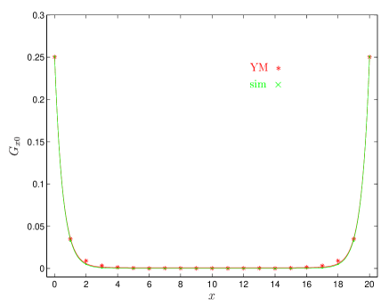
Figure 9: The Yang–Mills two–point function (YM) compared to the one obtained from the character action with 14 couplings (sim). Input: $\beta=2.20$, $N_{s}=20$.

These numerical values for $\lambda_{0}$ agree reasonably well with those of Table 8, where only four operators had been used. The benchmark test to be performed, however, is the calculation of the two–point function $G_{\mbox{\scriptsize\boldmath$x0$}}$ using the new effective couplings $g_{a}$. Fig.s 9 and 10 show that we have indeed improved the matching between Yang–Mills and the effective action.

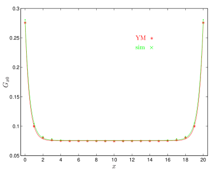
Figure 10: The Yang–Mills two–point function (YM) compared to the one obtained from the character action with 14 couplings (sim). Input: $\beta=2.40$, $N_{s}=20$.

This is quantitatively confirmed by repeating the fits of (95) and Table 10. The results displayed in Table 12 convincingly show the improvement in the effective action, in particular for the broken phase.

$\beta$		$a$	$b$	$c$
2.20	YM	$0.2493$	$1.9627$	$0.0009$
	sim	$0.2509$	$1.9837$	$0.0001$
2.40	YM	$0.2006$	$2.0715$	$0.0752$
	sim	$0.2051$	$1.9257$	$0.0758$

Table 12: Comparison of the fit parameters from (95) associated with Fig.s 9 and 10.

7 Summary and discussion

In this paper we have derived effective actions describing the dynamics of the (traced) Polyakov loop variable $L_{\mbox{\scriptsize\boldmath$x$}}\equiv\mbox{tr}\,\mathfrak{P}_{\mbox{\footnotesize\boldmath$x$}}/2$, and hence of the deconfinement phase transition. It has turned out useful, however, to regard the effective action as being derived from a more general theory depending on the untraced Polyakov loop $\mathfrak{P}_{\mbox{\footnotesize\boldmath$x$}}$ [17]. This theory is a nonlinear sigma model with target space $SU(2)\cong S^{3}$ and hence the symmetry $SU(2)\times SU(2)$ corresponding to left and right multiplication of $\mathfrak{P}_{\mbox{\footnotesize\boldmath$x$}}$ by group elements. Although the effective actions in $L$ clearly do not have this symmetry, it is nevertheless inherited by the functional Haar measure which implies novel Schwinger–Dyson equations for Polyakov loop correlators. In addition, it seems that a remnant of this symmetry shows up in the single–site distribution $p_{W}$ of $L_{\mbox{\scriptsize\boldmath$x$}}$ which is flat below $T_{c}$ meaning that $\mathfrak{P}_{\mbox{\footnotesize\boldmath$x$}}$ is distributed uniformly over the group manifold. Obviously, it would be desirable to really prove this equipartition for which we have found convincing numerical evidence. As the single–site distribution of $L_{\mbox{\scriptsize\boldmath$x$}}$ is exactly known in the confinement phase, we can give exact predictions for all moments $\langle L^{2k}\rangle$ and for the Binder cumulant, $b_{4}=-1$. Above $T_{c}$, we have fitted the log–distribution $W\sim\log p_{W}$ by polynomials so that also in this case we have good quantitative control of the distribution.

It turns out that $W[L]$ and a Ginzburg–Landau (or Svetitsky–Yaffe) effective action $S_{\mathrm{eff}}[L]$ are related in a manner that is simple enough to proceed by analytic means. Assuming that expectations taken in the effective action are unchanged if $L_{\mbox{\scriptsize\boldmath$x$}}$ is changed at a single site (another relation valid numerically but still subject to a proof) we have been able to express the effective couplings $\lambda_{2k}$ ($k\neq 0$) of $S_{\mathrm{eff}}[L]$ in terms of the parameters of $W$. The remaining coupling $\lambda_{0}$ is then determined by means of the Schwinger–Dyson equations. The single–site distributions resulting from the effective theory $S_{\mathrm{eff}}[L]$ agree very well with those obtained directly from Yang–Mills. Furthermore, the Svetitsky–Yaffe effective action perfectly fulfills the Schwinger–Dyson equations based on the $SO(4)$ invariance of the Haar measure.

For the symmetric phase ($T<T_{c}$) we have also determined the (constraint) effective potential from the single–site distribution $p_{W}$ assuming that the interactions are sufficiently short–ranged such that the law of large numbers may be invoked. As expected we obtain a Gaussian distribution for the mean field $\bar{L}$ if the volume is large and the temperature small enough.

By definition, one cannot calculate correlations from single–site distributions. Vice versa, the matching of these distributions does not imply that the correlation functions match as well. A direct comparison shows that the two–point functions of the Yang–Mills and Svetitsky–Yaffe ensembles differ somewhat, in particular in the broken phase. To improve the matching we have changed our operator basis from monomials in $L_{\mbox{\scriptsize\boldmath$x$}}$ to characters, which are orthogonal polynomials in $L_{\mbox{\scriptsize\boldmath$x$}}$. Technically, this results in a numerically rather stable inverse Monte Carlo procedure, even if the number of operators is large. We have obtained the effective couplings for a total number of 14 operators. The resulting effective theory has short–range interactions and reproduces the Yang–Mills two–point function in both phases very well.

Further research will be devoted to the following issues. The predictions of the effective actions for the dynamics of the phase transition should be investigated in detail. This includes an analysis of the effective potential(s) near and beyond the transition point as well as calculations of critical exponents. The latter will yield a check whether the effective action $S_{\mathrm{eff}}[L]$ is indeed in the universality class of the $\mathbb{Z}_{2}$–Ising–model. In addition, it should be possible to generalize the methods developed in this paper to higher $SU(N)$ gauge groups. Work in these directions is under way.

Appendix A Histograms and bins

Given a probability density $p_{W}[L]$ one defines the associated (cumulative) distribution function

$$P_{W}[L]\equiv\int_{-1}^{L}dL^{\prime}\,\sqrt{1-L^{\prime 2}}\;p_{W}[L^{\prime}]\;.$$ (106)

Density $p_{W}$ and distribution $P_{W}$ are related to our histograms as follows. We have a total number $N$ of ‘events’ or ‘measurements’ saying that a Polyakov loop at site $x$ belonging to an arbitrary configuration takes its value in some prescribed interval (‘bin’). Accordingly, $N$ is a fairly large number,

$$N=N_{s}^{3}\times N_{\mathrm{config}}=20^{3}\times 400=3.2\times 10^{6}\;.$$ (107)

The number of bins (labeled by integers $i$) is denoted by $I$, the number of events in bin $i$ by $C_{i}$. This number represents the height of the $i$th column in the histogram counting the absolute numbers of events with values in $[L_{i-1},L_{i}]$ . The relative counting rate is obtained by normalization,

$$c_{i}\equiv C_{i}/N=P_{W}[L_{i}]-P_{W}[L_{i-1}]=p_{W}[\bar{L_{i}}]\,\sqrt{1-\bar{L}_{i}^{2}}\;\Delta L_{i}\;,$$ (108)

where $\Delta L_{i}\equiv L_{i}-L_{i-1}$ and $\bar{L_{i}}\in[L_{i-1},L_{i}]$ chosen appropriately. The situation is depicted in Figure 11.

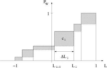
Figure 11: General histogram for distribution function $P_{W}[L]$.

Good statistics is achieved if the counting rate $c_{i}$ is approximately constant because then all bins will be equally ‘populated’. This can be achieved by suitably choosing the bin sizes $\Delta L_{i}$ which, however, is somewhat tricky because of the nontrivial measure in (106). If we ignore this for the moment and choose an equidistant partition,

$$\Delta L_{i}=\Delta L=2/I\;,$$ (109)

the total count in bin $i$ becomes

$$C_{i}=\frac{2N}{I}\,p_{W}[\bar{L}_{i}]\,\sqrt{1-\bar{L}_{i}^{2}}\;.$$ (110)

This yields rather bad statistics near the boundaries $L=\pm 1$, in particular for $T>T_{c}$, due to the suppression by the measure. For instance, choosing $\beta=2.4$, $I=100$, i.e. $\Delta L=1/50$, one typically finds $C_{1}\simeq 14000$ data points in the first bin (near $L=-1$), while the population of the bins near $L=0$ is larger by a factor of five, $C_{50}\simeq 73000$. The suppression by the geometry thus ‘wins’ against the density which is peaked near $L=\pm 1$. In the quantity of interest, the probability density,

$$p_{W}[\bar{L_{i}}]=\frac{C_{i}}{\sqrt{1-\bar{L}_{i}^{2}}}\,\frac{I}{2N}\;,$$ (111)

one divides by the measure factor which tends to zero near $L=\pm 1$. This yields the peaks near $L=\pm 1$ but at the same time further enhances the statistical error close to the boundaries. For $T<T_{c}$, this is not much of a problem as we have equipartition, $p_{W}[L]=const=p_{W}^{-}=2/\pi$, and the density is known anyhow. For $T>T_{c}$, however, (111) implies that the bulk of the density is located where the statistical error is largest. On the other hand, the behavior of $p_{W}$ in this regime determines the higher order couplings $\kappa_{2k}$. The lesson to be learned is that the partition should be modified such as to correctly incorporate the effect of the measure. To this end, we demand that the counting rate be constant, $c_{i}=c$, for $T<T_{c}$, hence, from (108),

$$c=p_{W}^{-}\,\sqrt{1-\bar{L}_{i}^{2}}\;\Delta L_{i}=1/I\;.$$ (112)

Thus, in order to properly take into account the measure, the bin size $\Delta L_{i}$ has to be chosen such that

$$\sqrt{1-\bar{L}_{i}^{2}}\;\Delta L_{i}=const=c/p_{W}^{-}=\frac{1}{Ip_{W}^{-}}\;.$$ (113)

This can be achieved by going over to continuum notation,

$$c/p_{W}^{-}=\int_{L_{i-1}}^{L_{i}}dL\,\sqrt{1-L^{2}}\equiv P_{W}[L_{i}]-P_{W}[L_{i-1}]\;,$$ (114)

and solving this recursion for $L_{i}$ numerically with $P_{W}(L)$ given by

$$P_{W}[L]=\frac{1}{2}\left[L\,\sqrt{1-L^{2}}+\arcsin(L)\right]\;.$$ (115)

Alternatively, one may produce an ordered list of all data points for $L$, and partition this list in such a way that all bins contain the same number $C$ of ‘events’. The sampling points $L_{i}$ are then given by the smallest (or largest, depending on the counting convention) value of $L$ in bin $i$.

For $T>T_{c}$, the density $p_{W}$ is then given by

$$p_{W}[\bar{L}_{i}]=\frac{Ip_{W}^{-}}{N}\,C_{i}\;.$$ (116)

This has been displayed in Figure 1. Obviously, measure effects are now absent and the difference between $C_{i}$ and $C$ represents the deviation from equipartition.

References

• [1] A. M. Polyakov, Thermal properties of gauge fields and quark liberation, Phys. Lett. B72 (1978) 477.
• [2] L. Susskind, Lattice models of quark confinement at high temperature, Phys. Rev. D20 (1979) 2610.
• [3] B. Svetitsky and L. Yaffe, Critical behavior at finite-temperature confinement transitions, Nucl. Phys. B210 (1982) 423.
• [4] L. G. Yaffe and B. Svetitsky, First-order phase transition in the SU(3) gauge theory at finite temperature, Phys. Rev. D26 (1982) 963.
• [5] M. Caselle and M. Hasenbusch, Deconfinement transition and dimensional cross-over in the 3d gauge Ising model, Nucl. Phys. B470 (1996) 435–453, [hep-lat/9511015].
• [6] F. Gliozzi and P. Provero, The Svetitsky-Yaffe conjecture for the plaquette operator, Phys. Rev. D56 (1997) 1131–1134, [hep-lat/9701014].
• [7] M. Pepe and P. de Forcrand, Finite size scaling of interface free energies in the 3-d Ising model, Nucl. Phys. B (Proc. Suppl.) 106 (2002) 914, [hep-lat/0110119].
• [8] P. de Forcrand and O. Jahn, Deconfinement transition in 2+1-dimensional SU(4) lattice gauge theory, hep-lat/0309153.
• [9] J. Polonyi and K. Szlachanyi, Phase transition from strong coupling expansion, Phys. Lett. B110 (1982) 395.
• [10] M. Okawa, Universality of the deconfining phase transition in (3+1)-dimensional SU(2) lattice gauge theory, Phys. Rev. Lett. 60 (1988) 1805.
• [11] S. Fortunato, F. Karsch, P. Petreczky, and H. Satz, Effective Z(2) spin models of deconfinement and percolation in SU(2) gauge theory, Phys. Lett. B503 (2001) 321, [hep-lat/0011084].
• [12] T. Banks and A. Ukawa, Deconfining and chiral phase transition in quantum chromodynamics at finite temperature, Nucl. Phys. B225 (1983) 145.
• [13] M. Ogilvie, Effective-spin model for finite-temperature QCD, Phys. Rev. Lett. 52 (1984) 1369.
• [14] B. Svetitsky, Symmetry aspects of finite-temperature phase transitions, Phys. Rept. 132 (1986) 1.
• [15] M. Caselle, Recent results in high-temperature lattice gauge theories, http://arXiv.org/abs/hep-lat/9601009. in: Selected Topics in Nonperturbative QCD, A. Di Giacomo and D. Diakonov, eds., Proceedings International School of Physics “Enrico Fermi”, Course CXXX, Varenna, Italy, 1995, IOS Press, Amsterdam, 1996.
• [16] M. Billo, M. Caselle, A. D’Adda, and S. Panzeri, Toward an analytic determination of the deconfinement temperature in SU(2) l.g.t, Nucl. Phys. B472 (1996) 163, [http://arXiv.org/abs/hep-lat/9601020].
• [17] R. Pisarski, Quark-gluon plasma as a condensate of $Z(3)$ Wilson lines, Phys. Rev. D62 (2000) 111501(R), [hep-ph/0006205].
• [18] P. Meisinger, T. Miller, and M. Ogilvie, Phenomenological equations of state for the quark-gluon plasma, Phys. Rev. D65 (2002) 034009.
• [19] H. Reinhardt, Resolution of Gauss’ law in Yang-Mills theory by gauge invariant projection: Topology and magnetic monopoles, Nucl. Phys. B503 (1997) 505, [hep-th/9702049].
• [20] C. Ford, U. G. Mitreuter, T. Tok, A. Wipf, and J. M. Pawlowski, Monopoles, Polyakov loops and gauge fixing on the torus, Ann. Phys. (N.Y.) 269 (1998) 26, [hep-th/9802191].
• [21] O. Jahn and F. Lenz, Structure and dynamics of monopoles in axial gauge QCD, Phys. Rev. D58 (1998) 085006, [hep-th/9803177].
• [22] G. ’t Hooft, Topology of the gauge condition and new confinement phases in non-Abelian gauge theories, Nucl. Phys. B190 (1981) 455.
• [23] K. Binder, Critical properties from Monte Carlo coarse graining and renormalization, Phys. Rev. Lett. 47 (1981) 693.
• [24] J. Fingberg, U. M. Heller, and F. Karsch, Scaling and asymptotic scaling in the SU(2) gauge theory, Nucl. Phys. B392 (1993) 493–517, [hep-lat/9208012].
• [25] M. Mathur, Landau Ginzburg model and deconfinement transition for extended SU(2) Wilson action, hep-lat/9501036.
• [26] H. Ursell, The evaluation of Gibbs’ phase integral for imperfect gases, Proc. Cambridge Phil. Soc. 23 (1927) 685.
• [27] J. Mayer, The statistical mechanics of condensing systems. I, J. Chem. Phys. 5 (1937) 67.
• [28] F. Coester and R. Haag, Representation of states in a field theory with canonical variables, Phys. Rev. 117 (1960) 1137.
• [29] H. Römer and T. Filk, Statistische Mechanik. VCH, Weinheim, 1994. (in German).
• [30] L. O’Raifeartaigh, A. Wipf, and H. Yoneyama, The constraint effective potential, Nucl. Phys. B271 (1986) 653.
• [31] D. Gross, R. Pisarski, and L. Yaffe, QCD and instantons at finite temperature, Rev. Mod. Phys. 53 (1981) 43.
• [32] N. Weiss, Effective potential for the order parameter of gauge theories at finite temperature, Phys. Rev. D24 (1981) 475.
• [33] Y. Fujimoto, H. Yoneyama, and A. Wipf, Symmetry restoration of scalar models at finite temperature, Phys. Rev. D38 (1988) 2625–2634.
• [34] M. Fukugita, M. Okawa, and A. Ukawa, Order of the deconfining phase transition in SU(3) lattice gauge theory, Phys. Rev. Lett. 63 (1989) 1768.
• [35] B. Svetitsky and N. Weiss, Ising description of the transition region in SU(3) gauge theory at finite temperature, Phys. Rev. D56 (1997) 5395.
• [36] P. Hasenfratz and F. Niedermayer, Perfect lattice action for asymptotically free theories, Nucl. Phys. B414 (1994) 785, [hep-lat/9308004].
• [37] A. Gottlob, M. Hasenbusch, and K. Pinn, Iterating block spin transformations of the O(3) non-linear sigma-model, Phys. Rev. D54 (1996) 1736–1747, [hep-lat/9601014].