Lattice QCD at Finite Density

Abstract

This is a pedagogical review of the lattice study of finite density QCD, which is intended to provide the minimum necessary contents, so that the paper may be used as the first reading for a newcomer to the field and also for those working in nonlattice communities. After a brief introduction to argue why finite density QCD can be a new attractive subject, we describe fundamental formulae which are necessary for the following sections.

Then we survey lattice QCD simulations in small chemical potential regions, where several prominent works have been reported recently. Next, two-color QCD calculations are discussed, where we have a chance to glance at many new features of finite density QCD, and indeed recent simulations indicated quark pair condensation and the in-medium effect. Tables of SU(3) and SU(2) lattice simulations at finite baryon density are given.

In the next section, we make a survey of several related works which may be a starting point of the new development in the future, although some works do not attract much attention now. Materials are described in a pedagogical manner. Starting from a simple 2-d model, we briefly discuss a lattice analysis of NJL model. We describe a non-perturbative analytical approach, i.e., strong coupling approximation method and some results. Canonical ensemble approach instead of usual grand canonical ensample may be another route to reach high density. We examine the density of state method and show this old idea includes recently proposed factorization method. An alternative method, complex Langevin equation and an interesting model, finite isospin model, are also discussed.

In the Appendix, we give several technical points which are useful in practical calculations.

1 Introduction

Finite density QCD (Quantum Chromodynamics) has attracted considerable attention in high energy physics, nuclear physics and astrophysics. Many theorists now believe that QCD has a very rich structure when we study it in temperature and density parameter space, and some experimentalists want to reveal it. Fig.1 shows a schematical phase diagram in $(T,\mu)$ plane. Lattice QCD has been expected to provide fundamental information about QCD in nonperturbative regions, and recently many promising works have appeared in this field.

In this paper, we discuss these activities together with a pedagogic introduction and related works. This is not a textbook-type comprehensive review. Minimum necessary knowledge and possible hints for future are given. Materials are taken from our notes, which we have been preparing during our research in this field. We hope this paper is a useful starting point for those who wish to join the field. For further reading, we cite several reviews. [1, 2, 3, 4, 5]

The most attractive possibility of finite density QCD is probably the color super conductivity (CSC). This was revealed first by one gluon exchange type calculation: Barrois, Bailin and Love, and Iwasaki and Iwado pointed out that an attractive force near the Fermi surface creates a Cooper pair, and results in CSC in the case of QCD at very low temperature and finite density [6]. In the late nineties, using the instanton type modeling of the attractive force, Alford, Rajagopal and Wilczek [7] and Rapp, Schaefer, Shuryak and Velkovsky [8] argued that the gap energy is of the order of 100 MeV, and therefore the transition temperature, which should be around the gap energy, is relatively high. In these arguments, two-flavor, i.e., $u$ and $d$ quark, color superconductivity is considered and termed 2CS. Fig.2 is a prediction of the phase by NJL model. [9]

Since these works, the field has been actively explored and there have been many interesting observations, e.g., at sufficiently large chemical potential, a state with a special combination of three flavors and color is stable and called color flavor locking (CFL) [10]; a new phase LOFF (Larkin, Ovchinnikov, Fulde and Ferrell), where pairing with different chemical potentials results in nonzero total momentum, may be favored [11]; the gap energy is $\sim\exp(-c/g)$ instead of $\sim\exp(-c/g^{2})$ [12] and so on. See Ref. RW. Introduction of Ref. PR also gives a good overview of the field.

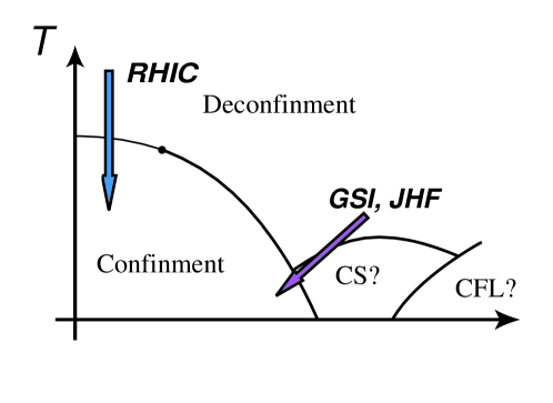
Figure 1: Schematic phase diagram of QCD in $(T,\mu)$ plane.

Figure 2: Phase diagram $(T,\mu)$ plane by NJL model. (Ref. NJL01).

Another interesting, but probably less well known possibility is chiral restoration in the nuclear medium. In the normal nuclear matter, the baryonic density is $\rho_{0}\sim 0.17/{\mbox{fm}}^{3}$. In a Nambu-Jona-Lashino (NJL) type model, the quark condensation, $\langle\bar{q}q\rangle$ at $\rho_{0}$ is less than that of the vacuum. We show the behavior of $\langle\bar{\psi}\psi\rangle$ as a function of $\mu$ and $T$ in a simple NJL model calculation in Fig.3. The quark condensation is an important parameter and causes many effects, such as vector meson masses. There are several recent experimental data which may yield information regarding in-medium hadrons,

• CERES: Large low mass $e^{+}e^{-}$ pair enhancement was observed in CERN SPS in Pb+Au collisions at 158 A GeV/c. This non trivial enhancement is also found at 40 AGeV/c where it is even larger, and the data may only be reproduced if the properties of the intermediate $\rho$ in the hot and dense medium are modified. [15]

• KEK: At KEK, invariant mass spectra of electron-positron pairs were measured in the region below the $\omega$ meson mass for the p+C and p+Cu collisions. The result was interpreted as being a signature of the $\rho/\omega$ modification at a normal nuclear-matter density. [16]

• STAR: The invariant mass of $\rho$ meson decays in Star experiment at $\sqrt{s}=200$ GeV Au+Au collisions at RHIC shows 60-70 MeV downward shift of the peak from its vacuum value. This suggests the modification of the spectral function at finite $T$ and $\mu$. [17]

• Pionic 1s states of Sn: Precision spectroscopy of pionic 1s states of Sn nuclei suggests $f^{*}_{\pi}(\rho_{0})^{2}/f_{\pi}^{2}=0.65\pm 0.05$, at the normal nuclear density. [18]

See Ref. Kunihiro for more detailed arguments and related theoretical and experimental works.

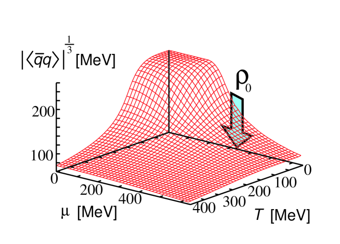
Figure 3: $\langle\bar{q}q\rangle$ as a function of $(T,\mu)$. We solve gap equations at finite temperature and density derived in Ref. LutzKlimtWeise92. We employ all parameter values given in LutzKlimtWeise92, except t$G_{D}$, which is set to be zero, i.e., we drop the s-quark contribution for simplicity. The arrow indicates the value of $\mu$ corresponding to the normal nuclear density $\rho_{0}$.

Hagedorn noted [21] that if the hadron spectrum increases exponentially,

$$\rho(m)=C{\rm e}^{m/T_{0}},$$ (1)

then the partition function diverges at some temperature $T_{c}$, called Hagedorn temperature,

$$\int dm\rho(m){\rm e}^{-m/T}=\infty\hskip 8.5359pt{\mbox{\rm if }}T>T_{0}.$$ (2)

Cabbibo and Parisi pointed out that the singularity of the partition function does not necessary mean the upper limit of the temperature, but the phase transition [22].

In 1981, McLerran and Svetitsky [23], and Kuti, Polonyi and Szlachanyi [24], demonstrated that when the temperature increases, a QCD matter encounters a phase transition from the confinement to the deconfinement phase by calculating Polyakov lines for two-color QCD. Since these pioneering works, lattice simulations have provided many detailed analyses of QCD at finite temperature. Still the order of the phase transition, i.e., the cross-over, the first or the second order, with the physical u, d and s quark masses is not yet finally determined. Lattice QCD is the first principle calculation, and can be considered as the most reliable starting point. See Ref. Kanaya02 for recent lattice investigations at finite temperature.

Then how about lattice QCD at finite density ? A lattice simulation of color SU(2) at finite temperature and density was carried out in 1984 and the transition from the confinement to the deconfinement state was observed [26]. Since then, to our knowledge, few lattice calculations were performed until 1999 [27, 28] except algorithmic study.

The reason is that when the chemical potential is introduced, the fermion determinant, $\det\Delta(\mu)$ becomes complex, which appears in the Euclidean path integral measure,

$$Z=\mbox{Tr}\,e^{-\frac{1}{kT}(H-\mu N)}=\int\mathcal{D}U\mathcal{D}\bar{\psi}\mathcal{D}\psi\,e^{-\frac{1}{kT}S_{G}-\bar{\psi}\Delta\psi}=\int\mathcal{D}U\det\Delta\,e^{-\frac{1}{kT}S_{G}}.$$ (3)

Here $\Delta$ is diagonal in flavor, $\Delta=\mbox{diag}(\Delta_{u},\Delta_{d},\Delta_{s},\cdots)$.

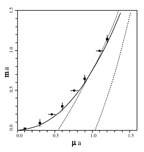
Figure 4: Phase diagram in the quark mass-chemical potential plane of the SU(3) gauge theory with staggered fermions at $\beta=0$ in the quench approximation. [29] The data points show the threshold value where physical observables start deviation from their $\mu=0$ values. The dotted line the expected critical line corresponding to the baryon threshold and the curve is the pion threshold which seems to describe the Monte Carlo data. The dotted curve is the result of the mean field calculation.

The simplest way to avoid the problem is to use the quench approximation, where we discard $\det\Delta(\mu)$. This approximation works well in many lattice calculations such as spectroscopy. However at the finite density it was found that the onset of chiral symmetry restoration occurs at a chemical potential of half the pion mass,

$$\mu_{c}=\frac{m_{\pi}}{2}$$ (4)

i.e., at the chiral limit, $\mu_{c}=0$. [29] Fig.4 shows data points in the quark mass-chemical potential plane at which physical observables start deviating from their $\mu=0$ values in quench simulations at $\beta=0$. The curve (dotted line) indicates the expected critical line correpoinding to pion (baryon) threshold.

Stephanov pointed out that quenched QCD is not the $N_{f}\to 0$ limit of QCD, but the limit of a theory with $2N_{f}$ quarks [30]. Let us consider the resolvent of the Dirac operator $\Delta$ for zero mass case,

$$G(x,y)=\langle\mbox{Tr}\frac{1}{z-\Delta}\rangle=\int dx^{\prime}dy^{\prime}\rho(x^{\prime},y^{\prime})\frac{1}{z-z^{\prime}},$$ (5)

where $z=x+iy$ is a complex variable. Banks-Casher relation is $\langle\bar{\psi}\psi\rangle=\pi\rho(0)$. $\rho$ can be inversely obtained as

$$\rho=\frac{1}{\pi}\frac{\partial G}{\partial z^{*}}.$$ (6)

Using the formula, $\det A=\exp\mbox{Tr}\log A$, we can write $G$ as

$$G=-\frac{\partial V}{\partial z},$$ (7)

where

$$V=-\langle\log\det(z-\Delta)\rangle.$$ (8)

If the standard replica trick works, $V$ can be obtained as $\lim_{n\rightarrow 0}V_{n}$, where

$$V_{n}=-\frac{1}{n}\log\langle{\det}^{n}(z-\Delta)\rangle.$$ (9)

Taking $\psi_{L,R}\equiv(1\pm\gamma_{5})/2\psi$ as bases, we can write $\Delta$ as

$$\Delta=\left(\begin{array}[]{cc}0&iX+\mu\\ iX^{\dagger}+\mu&0\end{array}\right)$$ (10)

where we employ the chiral representation of the Dirac matrices. Using the random matrix model where $X$ is treated as complex Gaussian random variables, Stephanov found that the above $V_{n}$ does not lead to the natural result, and we should start from $V_{n}$ which includes not only $z$ but also $z^{*}$,

$$V_{n}=-\frac{1}{n}\log\langle{\det}^{n}(z-\Delta)(z^{*}-\Delta^{\dagger})\rangle.$$ (11)

This corresponds to a system composed of $n$ quarks with original action and $n$ quarks with the conjugate action. Therefore to understand QCD at finite density, the quenched approximation is not appropriate and one needs dynamical simulations.

We have learned :

• QCD at finite density is an interesting attractive field of physics, and lattice QCD should play an important role here.

• Quench approximation of lattice QCD is not appropriate for the finite density system.

• Due to the complex nature of the fermion determinant $\det\Delta$, the standard Monte Carlo simulation is very difficult to obtain physical quantities.

In the following we continue our discussion, assuming the reader accepts these points.

In Sec.2, we give the fundamental formulae in lattice QCD at finite baryon density. In Sec.3, we describe recent prominent activities in small chemical potential and high temperature regions. In Sec.4, several numerical simulations of two-color QCD are reported, which suggest new interesting features at large $\mu$. In Sec.5, we collect several ideas and calculations which may give us a hint for the next step. We summarize and conclude our discussions in Sec. 6.

2 Formulation

A thermodynamical system is described by the partition function,

$$Z = {\rm{Tr}}({\rm e}^{-\frac{1}{kT}({H}-\mu{N})})$$ (12)

$$= \int\mathcal{D}U\mathcal{D}\bar{\psi}\mathcal{D}\psi{\rm e}^{-\int_{0}^{\beta}d\tau\int d^{3}x(L+\mu n)}$$

where $\beta=1/T$ and we impose the periodic (anti-periodic) boundary condition for $U$ ($\psi$) along the temporal direction [31] . The chemical potential is introduced in fermion action as $\mu\bar{\psi}\gamma_{0}\psi$. Therefore the fermion determinant has the form,

$$\Delta(\mu)=D_{\nu}\gamma_{\nu}+m+\mu\gamma_{0}.$$ (13)

Adopting anti-hermite $D$ and hermite $\gamma$ (final result does not depend on the representation.), we can easily show

$$\Delta(\mu)^{\dagger}=-D_{\nu}\gamma_{\nu}+m+\mu\gamma_{0}=\gamma_{5}\Delta(-\mu)\gamma_{5}$$ (14)

and then

$$(\det\Delta(\mu))^{*}=\det\Delta(\mu)^{\dagger}=\det\Delta(-\mu).$$ (15)

At $\mu=0$, this relationship guarantees that $\det\Delta$ is real.

In the continuum field theory, the chemical potential is introduced by the substitution,

$$p_{4}\rightarrow p_{4}-i\mu$$ (16)

in the fermion propagators. On the lattice with the lattice spacing $a$, the $\bar{\psi}\partial_{\mu}\psi$ term leads to $\bar{\psi}e^{ip_{\mu}a}\psi$. For example, a free propagator of Wilson fermions is given as,

$$\frac{1}{1-\kappa\sum_{\mu=1}^{4}\left\{(1-\gamma_{\mu})e^{ip_{\mu}a}+(1+\gamma_{\mu})e^{-ip_{\mu}a}\right\}}.$$ (17)

Therefore, we can naturally include the chemical potential exponentiated in the fermion matrix as,

$$\Delta(x,x^{\prime})=\delta_{x,x^{\prime}}-\kappa\sum_{i=1}^{3}\left\{(1-\gamma_{i})U_{i}(x)\delta_{x^{\prime},x+\hat{i}}+(1+\gamma_{i})U_{i}^{\dagger}(x^{\prime})\delta_{x^{\prime},x-\hat{i}}\right\}$$

$$-\kappa\left\{e^{+\mu}(1-\gamma_{4})U_{4}(x)\delta_{x^{\prime},x+\hat{4}}+e^{-\mu}(1+\gamma_{4})U_{4}^{\dagger}(x^{\prime})\delta_{x^{\prime},x-\hat{4}}\right\}.$$ (18)

For staggered (Kogut-Susskind) fermions,

$$\Delta(x,x^{\prime})=m\delta_{x,x^{\prime}}+\frac{1}{2}\sum_{i=1}^{3}\eta_{i}(x)\left\{U_{i}(x)\delta_{x^{\prime},x+\hat{i}}-U_{i}^{\dagger}(x^{\prime})\delta_{x^{\prime},x-\hat{i}}\right\}$$

$$+\frac{1}{2}\eta_{4}(x)\left\{e^{+\mu}U_{4}(x)\delta_{x^{\prime},x+\hat{4}}-e^{-\mu}U_{4}^{\dagger}(x^{\prime})\delta_{x^{\prime},x-\hat{4}}\right\},$$ (19)

where

$$\eta_{\mu}(x)=1\ (\mu=1),\ \ (-1)^{x_{1}}\ (\mu=2),\ \ (-1)^{x_{1}+x_{2}}\ (\mu=3),\ \ (-1)^{x_{1}+x_{2}+x_{3}}\ (\mu=4).$$ (20)

In other words, the chemical potential is introduced as,

$$U_{t}(x) \to e^{\mu}U_{t}(x),$$

$$U_{t}^{\dagger}(x) \to e^{-\mu}U_{t}^{\dagger}(x),$$ (21)

where $U_{\mu}(x)=\exp(iaA_{\mu}(x))$. Hasenfratz and Karsch have shown that the formula (21) avoids nonphysical divergence of the free energy of quarks [32]. Gavai considered more general form than $\exp(\pm\mu)$ in Eq.(21). [33] Creutz discussed how the chemical potential appears in lattice fermion formulation. [34]

The relation (14) holds for Wilson fermions, while in staggered fermion case, it is easy to check

$$\Delta(\mu)^{\dagger}=\Gamma_{5}\Delta(-\mu)\Gamma_{5},$$ (22)

where

$$\Gamma_{5}(x,x^{\prime})=(-1)^{x_{1}+x_{2}+x_{3}+x_{4}}\delta_{x,x^{\prime}}.$$ (23)

In the relativistic formulation, we expect the invariance under $\mu\rightarrow-\mu$. If we expand the partition function as

$$Z(\mu)=\sum_{k}\frac{\mu^{k}}{k!}\frac{\partial^{k}}{\partial\mu^{k}}\int\mathcal{D}U\det\Delta e^{-\beta S_{G}}|_{\mu=0},$$ (24)

the terms with odd power of $\mu$ vanish. Let us check $k=1$ case explicitly; At $\mu=0$,

$$\frac{\partial}{\partial\mu}\det\Delta=\mbox{Tr}[\Delta^{-1}\frac{\partial\Delta}{\partial\mu}]\det\Delta=\mbox{Tr}[\gamma_{5}\Delta^{-1}\gamma_{5}\gamma_{5}\frac{\partial\Delta}{\partial\mu}\gamma_{5}]\det\gamma_{5}\Delta\gamma_{5}$$

$$=\mbox{Tr}[\Delta^{\dagger-1}(-\frac{\partial\Delta^{\dagger}}{\partial\mu})]\det\Delta^{\dagger}=-\mbox{Tr}[\Delta(U^{\dagger})^{-1}\frac{\partial\Delta(U^{\dagger})}{\partial\mu}]\det\Delta(U^{\dagger}),$$ (25)

where we use Eq.(14). The integration measure $\mathcal{D}U$ and the gluon action $S_{G}$ are invariant under the change $U\rightarrow U^{\dagger}$, we get $\partial Z/\partial\mu=-\partial Z/\partial\mu=0$ at $\mu=0$.

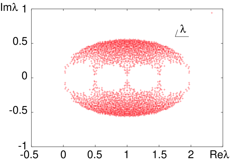
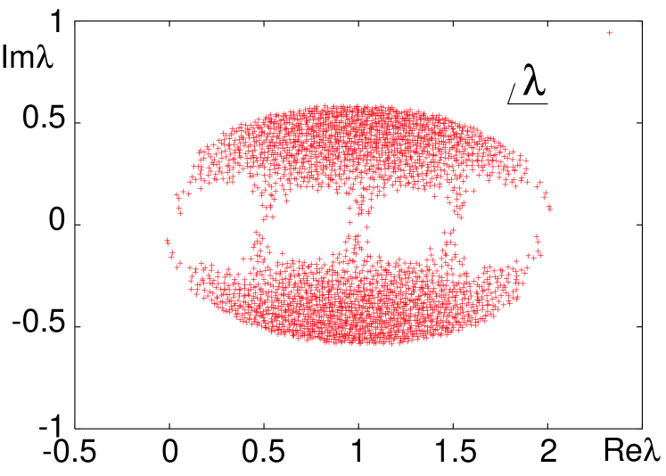
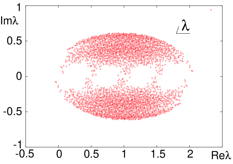
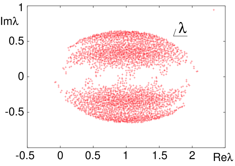
Figure 5: Eigen value distribution. Wilson fermions. $4^{4}$ lattice. $ma=0.1$. Quench $\beta=5.7$.

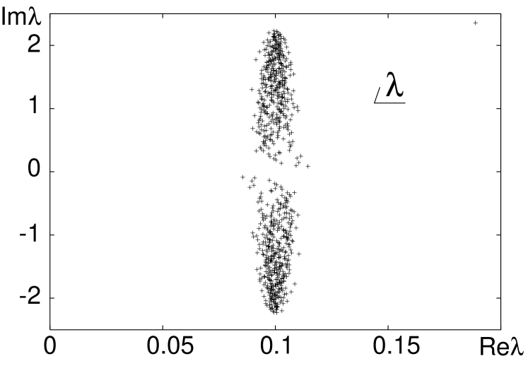
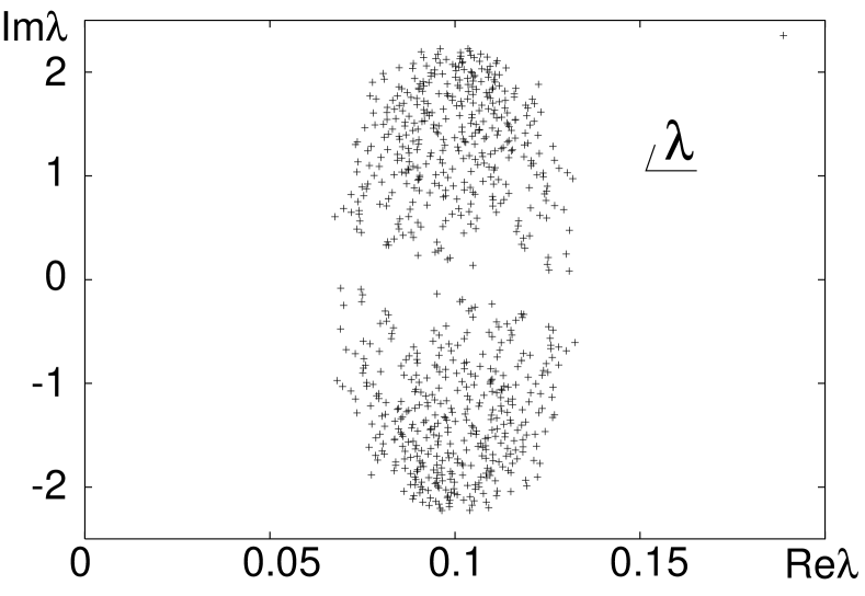
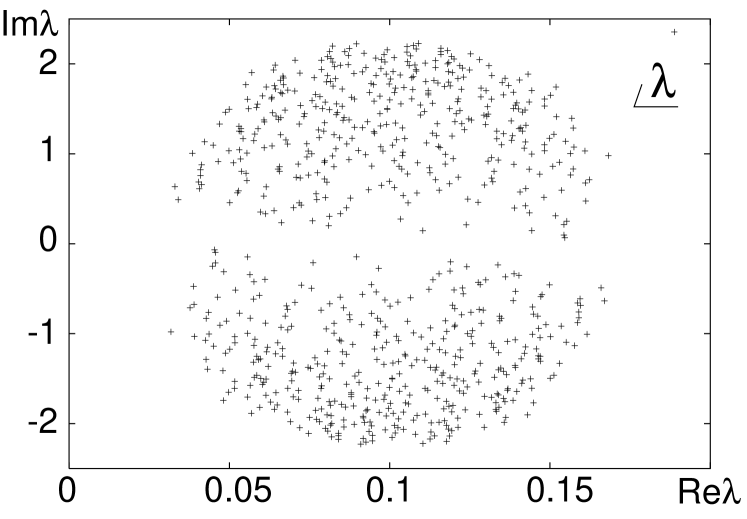
Figure 6: Eigen value distribution. Staggered fermions. $4^{4}$ lattice. $ma=0.1$. Quench $\beta=5.7$.

We show in Figs.5 and 6 typical eigen value distributions for Wilson fermions (Fig.5) and staggered fermions (Fig.6). Here configurations are generated in the quench approximation, since so far there is no algorithm which enables us to calculate the path integral (3) at finite $\mu$.

It is sometimes convenient to change variables, $\psi$ and $\bar{\psi}$ as

$$\psi(\vec{x},t_{i})\rightarrow e^{-t_{i}\mu}\psi(\vec{x},t_{i})$$

$$\bar{\psi}(\vec{x},t_{i})\rightarrow e^{+t_{i}\mu}\bar{\psi}(\vec{x},t_{i})$$ (26)

where $t_{i}=1,2,\cdots,N_{t}$. Then

$$\bar{\psi}(\vec{x},t_{i})e^{\mu}U_{t}(\vec{x},t_{i})\psi(\vec{x},t_{i+1})\rightarrow\bar{\psi}(\vec{x},t_{i})U_{t}(\vec{x},t_{i})\psi(\vec{x},t_{i+1})$$ (27)

i.e., we do not need to put a factor $e^{\pm\mu}$ to the link variables, $U_{t}$ and $U^{\dagger}_{t}$, except at the temporal edge of the lattice where

$$e^{N_{t}\mu}U_{t}(\vec{x},N_{t}) = e^{\mu/T}U_{t}(\vec{x},N_{t})$$

$$e^{-N_{t}\mu}U_{t}^{\dagger}(\vec{x},N_{t}) = e^{-\mu/T}U_{t}^{\dagger}(\vec{x},N_{t}).$$ (28)

The partition function should be a function of $N_{t}\mu=\beta\mu=\mu/T$ (see Eq.(3)), therefore the above expressions appear to be natural.

3 Three Color

Even though the fermion determinant $\det\Delta$ is complex, one may perform Monte Carlo simulations by taking its modulus as a measure,

$$\langle O\rangle = \frac{1}{Z}\int\mathcal{D}U\,O\,\det\Delta\,e^{-\beta S_{G}}=\frac{\int\mathcal{D}U\,O\,|\det\Delta|e^{i\theta}\,e^{-\beta S_{G}}}{\int\mathcal{D}U|\det\Delta|e^{i\theta}\,e^{-\beta S_{G}}}$$ (29)

$$= \frac{\int\mathcal{D}U\,O\,|\det\Delta|e^{i\theta}\,e^{-\beta S_{G}}}{\int\mathcal{D}U|\det\Delta|\,e^{-\beta S_{G}}}\displaystyle{/}\frac{\int\mathcal{D}U|\det\Delta|e^{i\theta}\,e^{-\beta S_{G}}}{\int\mathcal{D}U|\det\Delta|\,e^{-\beta S_{G}}}$$

$$= \frac{\langle Oe^{i\theta}\rangle_{0}}{\langle e^{i\theta}\rangle_{0}}$$

where $\langle\cdots\rangle_{0}$ is the expectation value with $|\det\Delta|$ as the measure, i.e., phase quenching measure. The direct calculations were pursued on small lattices, but a large phase fluctuation hinders us from obtaining a meaningful signal in low temperature and large chemical potential regions, i.e., the numerator and denominator of the last term of Eq.(29) are very small [35, 36, 37]. Lattice QCD at finite chemical potential suffers from a severe sign problem. In spite of this difficulty, there have been many challenging efforts, which we will survey in this section. Table 1 is a compilation of numerical simulations of three color system.

Table 1: Three Color

Action	parameters	comments	Ref.
Plaq. + KS	$N_{f}=2$, $m_{q}=0.00625,0.0125$, $16^{3}\times 8$	quark number susceptibility	Gott
Plaq. + KS	$N_{F}=2$, $m_{q}=0.0125,0.0170,0.0250$, $16\times 8^{2}\times 4$	response of observables at $\mu=0$	QCD-Taro02
Plaq. + KS	$N_{f}=2+1$, $m_{u,d}=0.025$, $m_{s}=0.2$, $N_{s}^{3}\times 4$, $N_{s}=$ 8,10,12	phase diagram, q method	FodorKatz
Imp. + Imp. KS	$N_{f}=2$, $m_{q}=0.1,0.2$, $16^{3}\times 4$	Taylor expansion, reweighting method	Allton
Imp. + Imp. KS	$N_{f}=2$, $m/T=0.1$, 0.4, $16^{3}\times 4$	Taylor expansion, analytic frame work, equation of state	Allton03
Plaq. + KS	$N_{f}=4$, $m_{q}=0.05$, $16^{3}\times 4$	imaginary chemical potential	DElia
Plaq. + KS	$N_{f}=2$, $m_{q}=0.025$, $8^{3}\times 4$, $6^{3}\times 4$	QCD phase diagram, imaginary chemical potential	FP
Plaq. + KS	$N_{f}=2+1$, $m_{u,d}=0.025$, $m_{s}=0.2$, $N_{s}^{3}\times 4,N_{s}=$ 8,10,12	equation of state	FodorKatz2

3.1 Response of observables with respect to $\mu$ at $\mu=0$

Although the direct simulations at finite $\mu$ is very hard, one may measure the effect of the chemical potential through the response of physical observables with respect to the chemical potential at $\mu=0$. Such an attempt was first pursued by Gottlieb et. al.[38].

They calculated the singlet and non-singlet quark number susceptibilities, $\chi_{S}(+)$ and $\chi_{NS}(-)$,

$$\chi_{S,NS}=\left(\frac{\partial}{\partial\mu_{u}}\pm\frac{\partial}{\partial\mu_{d}}\right)(n_{u}\pm n_{d})$$ (30)

where $n_{i}$ for $i=u,d$ is the quark number densities given by

$$n_{i}=\frac{T}{V}\frac{\partial\log Z}{\partial\mu_{i}}$$ (31)

These susceptibilities are found to be very small in the low temperature phase and to increase abruptly at the transition temperature. The two susceptibilities are almost same, e.g. $\chi_{S}\approx\chi_{NS}$ which indicates that fluctuations in the $u$ and $d$ quark densities are uncorrelated. These susceptibilities are important since they are related to event-by-event fluctuations and diffusion in relativistic heavy-ion collisions[47]. Further studies in the susceptibilities for quenched and 2 flavors QCD can be found in [48, 49, 50, 51]. MILC (MIMD Lattice Computation) collaboration recently calculated the susceptibilities for three flavors with improved staggered fermions.[52] Fig.7 shows the triplet susceptibility $\chi_{trip}(=\chi_{NS}$ here) on $8^{3}\times 4$, $12^{3}\times 6$ and $16^{3}\times 8$ lattices and indicates the excellent scaling properties between the $N_{t}=6$ and $N_{t}=8$ results. Fig.8 shows the difference between singlet and triplet susceptibility. One can see the clear difference between the two susceptibilities around the phase transition which occurs at about 180 MeV.

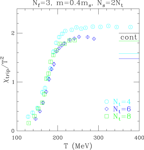
Figure 7: The triplet quark number susceptibility fo $N_{f}=3$ on $8^{3}\times 4$, $12^{3}\times 6$ and $16^{3}\times 8$ lattices.

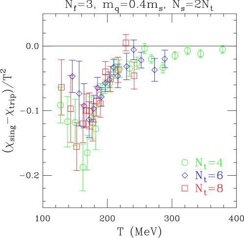
Figure 8: The difference between singlet and triplet quark number susceptibility for $N_{f}=3$ on $8^{3}\times 4$, $12^{3}\times 6$ and $16^{3}\times 8$ lattices.

QCD-TARO (Thousand-cell ARray processors for Omni-purposes) collaboration has extended the idea of Ref.[38] further and calculated derivatives of meson screening masses and the quark condensation with respect to the chemical potential at $\mu=0$.[39] Consider a meson propagator $C(z)$ in $z$ direction consisting of $u$ and $d$ quarks as an example,

$$C(z) = A(e^{-Mz}+e^{M(L_{z}-z)})$$

$$= \frac{1}{Z}\int\mathcal{D}U\,H(z)H^{\dagger}(0)\,\,e^{-\beta S_{G}-\bar{\psi}\Delta\psi}$$

$$= \frac{1}{Z}\int\mathcal{D}UG(z)\det\Delta\,e^{-\beta S_{G}},$$ (33)

where $H(x)=\bar{\psi}(x)\Gamma\psi(x)$ is a meson operator and

$$G(z)\equiv\mbox{Tr}\Gamma\Delta_{u}^{-1}(z,0)\Gamma\Delta_{d}^{-1}(0,z).$$ (34)

We neglect possible higher states for simplicity.

The first derivative of $C(z)$ with respect to the chemical potential leads to

$$\frac{1}{C(z)}\frac{dC(z)}{d\mu}=\frac{1}{A}\frac{dA}{d\mu}+\frac{dM}{d\mu}\left\{\left(z-\frac{L_{z}}{2}\right)\tanh\left[M\left(z-\frac{L_{z}}{2}\right)\right]-\frac{L_{z}}{2}\right\}.$$ (35)

Similarly the second derivative is given as

$$\frac{1}{C(z)}\frac{d^{2}C(z)}{d\mu^{2}} = \frac{1}{A}\frac{d^{2}A}{d\mu^{2}}\left(\frac{2}{A}\frac{dA}{d\mu}\frac{dM}{d\mu}+\frac{d^{2}M}{d\mu^{2}}\right)\times\left\{\left(z-\frac{L_{z}}{2}\right)\tanh\left[M\left(z-\frac{L_{z}}{2}\right)\right]-\frac{L_{z}}{2}\right\}$$ (36)

$$+ \left(\frac{dM}{d\mu}\right)^{2}\left\{\left(z-\frac{L_{z}}{2}\right)^{2}+\frac{L_{z}^{2}}{4}-L_{z}\left(z-\frac{L_{z}}{2}\right)\tanh\left[M\left(z-\frac{L_{z}}{2}\right)\right]\right\}.$$

The numerical data of the derivative of $C(z)$ to $\mu$ is given as follows.

$$\frac{dC(z)}{d\mu}=\frac{d<G(z)>}{d\mu}=\left\langle\dot{G}+G\frac{\dot{D}}{D}\right\rangle-\langle G\rangle\left<\frac{\dot{D}}{D}\right\rangle,$$ (37)

$$\frac{d^{2}<G(z)>}{d\mu^{2}}=\left\langle\ddot{G}+2\dot{G}\frac{\dot{D}}{D}+G\frac{\ddot{D}}{D}\right\rangle-2\left\langle\dot{G}+G\frac{\dot{D}}{D}\right\rangle\left<\frac{\dot{D}}{D}\right\rangle-\langle G\rangle\left\{\left<\frac{\ddot{D}}{D}\right>-2\left\langle\frac{\dot{D}}{D}\right\rangle^{2}\right\},$$ (38)

where $D$ stands for $\det\Delta$ and the dotted $\dot{O}$ and $\ddot{O}$ denote the first and the second derivatives of an operator $O$ with respect to $\mu$. Fitting the numerical data of Eqs.(37) and (38) to Eqs.(35) and (36) we can determine the derivatives of the residue $A$ and the meson mass $M$. Thus with the derivatives of $M$, we can obtain the behavior of a hadron mass in the vicinity of $\mu=0$ as a function of the chemical potential,

$$M(\mu)=M(0)+\mu\left.\frac{\partial M}{\partial\mu}\right|_{\mu=0}+\left.\frac{1}{2}\mu^{2}\frac{\partial^{2}M}{\partial\mu^{2}}\right|_{\mu=0}+\cdots$$ (39)

The first derivative of the pseudo-scalar (PS) mass turned out to be consistent with zero $\mu=0$. In Fig.9, we show the second derivative of the PS mass where iso-scalar and iso-vector type chemical potentials, $\mu_{S}$ and $\mu_{V}$, are introduced,

$$\mu_{S} \equiv \mu_{u}=\mu_{d},$$

$$\mu_{V} \equiv \mu_{u}=-\mu_{d}.$$ (40)

In the low temperature phase the second derivative of the PS mass $M$ with respect to $\mu_{S}$ is small. This is expected since below the critical temperature and in the vicinity of zero $\mu_{S}$, the PS meson still keeps a property as a Goldstone boson and persists its behavior. On the other hand, above $T_{c}$, the PS meson is no longer a Goldstone boson and the second derivative of $M$ seems to remain finite. In contrast to the case of $\mu_{S}$ the second derivative of $M$ with respect to $\mu_{V}$ is significantly large in the low temperature phase and decreases in magnitude above $T_{c}$.

Figure 9: The second derivative of the pseudo scalar mass $\left.\frac{d^{2}M}{d\mu^{2}}\right|_{\mu=0}$ for isoscalar and isovector chemical potentials, $\mu_{S}$ and $\mu_{V}$. (Ref. QCD-Taro02).

As we will see later, the fermion determinant with the isovector chemical potential is equivalent to that of a two-flavor system without the phase. Large nonzero values of the second derivative of the pseudo-scalar meson mass may suggest some phase structure in finite but small chemical potential regions. Son and Stephanov have shed a new light on the model as a finite isospin density system. See section 5.7.

Gavai and Gupta calculated the depedence of the pressure $P$ on $\mu$ through a Taylor expansion at $\mu=0$.[53] For a homogeneous system, the pressure $P$ is obtained by $P=-F/V$, where $F=-T\log Z$. Therefore the Taylor expansion of $P$ at $\mu_{i}=0$ ($i=u$,$d$,…) is given by

$$P(\mu_{u},\mu_{d},...) = P(0)-\frac{1}{V}\sum_{i}\frac{\partial F}{\partial\mu_{i}}-\frac{1}{2V}\sum_{i,j}\frac{\partial^{2}F}{\partial\mu_{i}\partial\mu_{j}}+...$$ (41)

$$= P(0)+\sum_{i}\chi_{i}+\sum_{i,j}\chi_{ij}+...$$ (42)

The second term $\chi_{i}$ corresponds to the quark number density which is zero at $\mu=0$ and the third therm $\chi_{ij}$, the quark number susceptibility. One can consider the higher order derivative terms and all the odd derivatives vanish by CP symmetry. The Taylor series of $P$ up to the fourth order for $\mu_{u}=\mu_{d}=\mu$ is given by

$$\frac{\Delta P}{T^{4}}=\left(\frac{\chi_{uu}}{T^{2}}\right)\left(\frac{\mu}{T}\right)^{2}\left[1+\left(\frac{\mu/T}{\mu_{*}/T}\right)^{2}\right]$$ (43)

where $\Delta P=P(\mu)-P(0)$, and

$$\frac{\mu_{*}}{T}=\sqrt{\frac{12\chi_{uu}/T^{2}}{|\chi_{uuuu}|}}$$ (44)

$\chi_{uudd}$ is neglected since it turns out to be numerically smaller than the errors in $\chi_{uuuu}$. Fig.10 shows $\frac{\Delta P}{T^{4}}$ obtained in quenched QCD. For $\mu/T_{c}=0.15$, the effects of $\mu$ on $P$ are very small, which implies that at RHIC region where $\mu/T_{c}\sim 0.06$, the effects are also small. As $\mu/T_{c}$ increases, the effects become significant. One could see the effects at SPS region where $\mu/T_{c}\sim 0.45$.

Figure 10: $\displaystyle\frac{\Delta P}{T^{4}}$ as a function of $T/T_{c}$ for the values of $\mu/T_{c}$.

3.2 Glasgow approach

The Glasgow group has been developing the way towards simulations of lattice QCD at finite density. See Ref. barbour98 and references therein.

Consider the partition function at $\mu$ normalized by that of $\mu=0$.

$$Z = \frac{\int\mathcal{D}U\det\Delta(\mu)\,e^{-\beta S_{G}}}{\int\mathcal{D}U\det\Delta(0)\,e^{-\beta S_{G}}}=\frac{\int\mathcal{D}U\frac{\det\Delta(\mu)}{\det\Delta(0)}\det\Delta(0)\,e^{-\beta S_{G}}}{\int\mathcal{D}U\det\Delta(0)\,e^{-\beta S_{G}}}$$ (45)

$$= \left\langle\frac{\det\Delta(\mu)}{\det\Delta(0)}\right\rangle_{\mu=0}=\sum_{n=-3N_{s}^{3}}^{+3N_{s}^{3}}\langle b_{|n|}\rangle_{\mu=0}\,e^{n\mu/T}$$

Taking the derivative of $Z$ with respect to $T$ and $\mu$, we obtain the energy and the baryon number density, respectively. By investigating zeros in the complex $\mu$-plane,

$$Z(\mu)=0$$ (46)

we have Lee-Yang zero. It was very difficult to obtain reliable values of $\langle b_{|n|}\rangle$ numerically at low temperature when $\mu$ increases.

3.3 Reweighting by Fodor and Katz

Fodor and Katz [40] have achieved a great step in lattice QCD simulation at finite density, i.e., they have for the first time succeeded in estimating the phase transition line at finite $\mu$ in $(T,\mu)$ parameter plane. See Fig.11.

They proposed using the multi-parameter reweighting method. The essential idea is to use the gauge coupling constant $\beta$ as a controlling parameter,

$$\langle O\rangle = \frac{1}{Z(\mu)}\int\mathcal{D}U\,O\,\det\Delta(\mu)\,e^{-\beta S_{G}}$$ (47)

$$= \frac{1}{Z(\mu)}\int\mathcal{D}U\,O\,\frac{\det\Delta(\mu)}{\det\Delta(0)}\,e^{-(\beta-\beta_{0})S_{G}}\det\Delta(0)\,e^{-\beta_{0}S_{G}}$$

$$= \frac{\langle O\frac{\det\Delta(\mu)}{\det\Delta(0)}e^{-\Delta\beta S_{G}}\rangle_{0}}{\langle\frac{\det\Delta(\mu)}{\det\Delta(0)}e^{-\Delta\beta S_{G}}\rangle_{0}}$$

and choose $\beta_{0}$ so that

$$\left|\frac{\det\Delta(\mu)}{\det\Delta(0)}\right|e^{-\Delta\beta S_{G}}$$ (48)

becomes as large as possible, i.e., the overlap should be large. In Eq.(47) , $\langle\cdots\rangle_{0}$ stands for the evaluation at $(\beta_{0},\mu=0)$. The coupling constant $\beta_{0}$ is taken at the confinement/deconfinement transition point, and physical quantities near the phase transition line are calculated by the formula (47), i.e., quantities on the phase transition line in $(T,\mu)$ plane are evaluated at $(T_{c},\mu=0)$ with the reweighting factor. A possible interpretation for this procedure is that points on the phase transition line have similar nature. (Fig.12)

If the reweighting factor, (48), is large, we can get better signal. Further if in some regions of $(\mu,\beta)$ parameter space, this value changes little, we have similar reweighting effect there. Ejiri investigated the problem, and observed that the chemical potential effect through the phase of the fermion matrix does not contribute to the $\beta$ dependence of the gauge action, and $\mu$ in the amplitude, $|\det\Delta(\mu)|$, correlates strongly with $e^{-\Delta\beta S_{G}}$. [56]

Figure 11: Phase diagram obtained by Fodor and Katz. (Ref. FodorKatz)

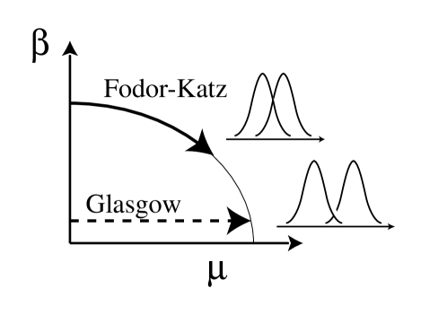
Figure 12: Schematic diagram of multi-parameter reweighting.

In this calculation we need the ratio of the determinant, $\det\Delta(\mu)/\Delta(0)$. Gibbs obtained a useful formula, [55]

$$\det\Delta(\mu)=e^{N_{t}V_{s}\mu}\prod_{i=1}^{6V_{s}}(\lambda_{i}+e^{-N_{t}\mu}),$$ (49)

where $\lambda_{i}$ are eigen values of a matrix constructed from the spatial and mass terms of fermion matrix, which does not depend on the chemical potential $\mu$. Therefore once we obtain the eigenvalues $\lambda_{i}$, we can calculate the determinant at any $\mu$ for a fixed gauge field. See Appendix A.

Note that, though Fodor and Katz obtained great success near the phase transition line, they did not solve the sign problem of the finite density lattice QCD. It still remains difficult to study a low-temperature region where the phase fluctuation coming from the complex fermion determinant is most probably large. Fig.13 shows $\langle\cos\theta\rangle$ as a function of $\mu$ obtained by Bielefeld-Swansea group for various $beta$ and quark masses. At large $\mu$, the complex phase of the fermion determinant becomes large, i.e., the nominator and denominator in Eq.29 are small.

Figure 13: The phase of complex determinant calculated by Bielefeld-Swansea collaboration. (Ref. Allton).

3.4 Taylor expansion

Fodor and Katz calculated determinants in Eq.(47), but it is difficult to study large lattices by the present computers. In any case, we cannot study large chemical potentials because of the sign problem.

Bielefeld-Swansee collaboration[41] proposed using Taylor expansion at $\mu=0$,

$$\ln\left(\frac{\det\Delta(\mu)}{\det\Delta(0)}\right)=\sum_{n=1}^{\infty}\frac{\mu^{n}}{n!}\frac{\partial^{n}\ln\det\Delta}{\partial\mu^{n}}$$ (50)

At the lowest order, the phase of the determinant is obtained as $\displaystyle\mu{\rm Im}{\rm Tr}M^{-1}\frac{\partial M}{\partial\mu}$ which is easier to evaluate than the direct calculation from the determinant itself.

Figure 14: Phase diagram obtained by Bielefeld-Swansea collaboration. (Ref. Allton).

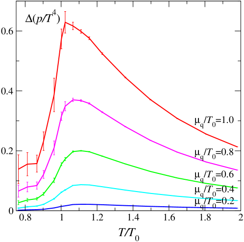
Figure 15: The equation of state correction $\Delta(p/T^{4})$ vs. $T/T_{c0}$ for various $\mu/T_{c0}$ by Bielefeld-Swansea collaboration. (Ref. Allton03).

Employing the formula, they have performed thorough studies in small $\mu$ regions which cover RHIC experiments and obtained the phase diagram similar to that of Fodor and Katz.

Recently they study the thermodynamical grand potential up to the fourth order of the derivative with respect to the chemical potential, and calculate the quation of state. Allton03 Fig.15 shows $\Delta(p/T^{4})$ which is defined as

$$\Delta\left(\frac{p}{T^{4}}\right)\equiv\left.\frac{p}{T^{4}}\right\|_{T,\mu}-\left.\frac{p}{T^{4}}\right\|_{T,0}.$$ (51)

The correction of the pressure is large for $0.9\leq T/T_{0}\leq 1.3$, $\mu/T_{0}\geq.5$, but will decrease as $T$ rises further. Fodor, Katz and Szabo reported similar result. FodorKatzSzabo

3.5 Imaginary chemical potential

If the chemical potential is pure imaginary, i.e., $\mu=i\mu_{I}$, then the fermion matrix $\Delta$ becomes,

$$\Delta=D_{\nu}\gamma_{\nu}+m+i\mu_{I}\gamma_{0}$$ (52)

and

$$\Delta^{\dagger}=\gamma_{5}\Delta\gamma_{5}.$$ (53)

Thus $\det\Delta$ with a pure imaginary chemical potential is real.

If we use the expressions 28 in section 2, the link variable at $t=N_{t}$ has the form,

$$e^{i\frac{\mu_{I}}{T}}U_{t}(\vec{x},N_{t}).$$ (54)

As is well known, the gauge action $S_{G}$ has $Z_{3}$ symmetry, i.e., $S_{G}$ is invariant when link variables on a time slice change as

$$U_{t}\rightarrow zU_{t}$$ (55)

where $z$ is an element of $Z_{3}$ group,

$$z=e^{i\phi},\qquad\phi=0,\frac{2\pi}{3},\frac{4\pi}{3}.$$ (56)

But the fermion action is not invariant under the transformation.

In the case of the imaginary chemical potential, the $Z_{3}$ transformation of the link variables can be absorbed into $\mu_{I}$ in the fermion action. Conversely, the shift of the imaginary chemical potential,

$$\mu_{I}\rightarrow\mu_{I}+\phi$$ (57)

can be managed as the change of the link variables, $U_{t}\to zU_{t}$, which can be regarded as the simple change of the integration variables $U_{t}$ to $zU_{t}$. Therefore, the path integral gives the same result,

$$Z(\mu_{I}+\phi)=Z(\mu_{I}).$$ (58)

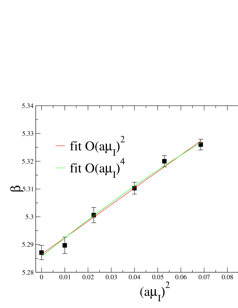
Figure 16: Imaginary chemical potential study by de Forcrand and Philipsen. Critical $\beta_{c}$ obtained with the imaginary chemical potential $\mu_{I}$ is fitted by $\beta_{c}(a\mu_{I})=c_{0}+c1(a\mu_{I})^{2}$ (left), and converted through ${\rm{Im}}\mu=-i{\rm{Re}}\mu$ to obtain the critical lines in $(T,\mu)$ (right). (Ref. FP).

Under this constraint, we can perform the analytic continuation of the results obtained with $\mu_{I}$ to the real $\mu$. The idea has been known for many years, and recently de Forcrand and Philipsen, and D’Elia and Lombardo have successfully performed simulations. In Ref. FP, the critical $\beta$ is fitted as

$$\beta=a_{0}+a_{2}\mu_{I}^{2}+\cdots$$ (59)

and transformed to the real chemical potential,

$$\beta=a_{0}-a_{2}\mu^{2}+\cdots$$ (60)

The result is shown in Fig.16.

Imaginary chemical potential may be considered as a special boundary condition.

4 Two Color

Since SU(2) matrix $U$ has the following property,

$$U_{\mu}^{*}=\sigma_{2}U_{\mu}\sigma_{2},$$ (61)

$$\Delta(U,\gamma_{\mu})^{*}=\Delta(U^{*},\gamma_{m}u^{*})\sigma_{2}\Delta(U,\gamma_{m}u^{*})\sigma_{2},$$ (62)

then $\{\det\Delta(x,x^{\prime};\gamma_{\mu})\}^{*}=\det\Delta(x,x^{\prime};\gamma_{\mu}^{*})$. $\gamma_{\mu}^{*}$ are a representation which satisfies the anti-commutation relations as $\gamma_{\mu}$ and $\det\Delta$ should not depend on the representation. Consequently,

$$\det\Delta(x,x^{\prime};\gamma_{\mu})^{*}=\det\Delta(x,x^{\prime};\gamma_{\mu})$$ (63)

i.e., the fermion determinant is real. For reader’s convenience, we show a compilation of color SU(2) finite density simulations in Table 2.

In Refs. KSteT and KSTVZ, the authors have determined the lowest order, i.e., $O(E^{2})$, effective Lagrangian including the chemical potential,

$${\cal L}_{\rm eff} = {F^{2}\over 2}{\rm Tr}\partial_{\nu}\Sigma\partial_{\nu}\Sigma^{\dagger}+2\mu F^{2}{\rm Tr}B\Sigma^{\dagger}\partial_{0}\Sigma$$ (64)

$$\hskip 10.00002pt-F^{2}\mu^{2}{\rm Tr}\left(\Sigma B^{T}\Sigma^{\dagger}B+BB\right)-F^{2}m_{\pi}^{2}{\rm Re}{\rm Tr}\left(\hat{M}\Sigma\right).$$

where

$$B\equiv\left(\begin{array}[]{cc}+1&0\\ 0&-1\end{array}\right)$$ (65)

$$\hat{M}\equiv\left(\begin{array}[]{cc}0&1\\ -1&0\end{array}\right)$$ (66)

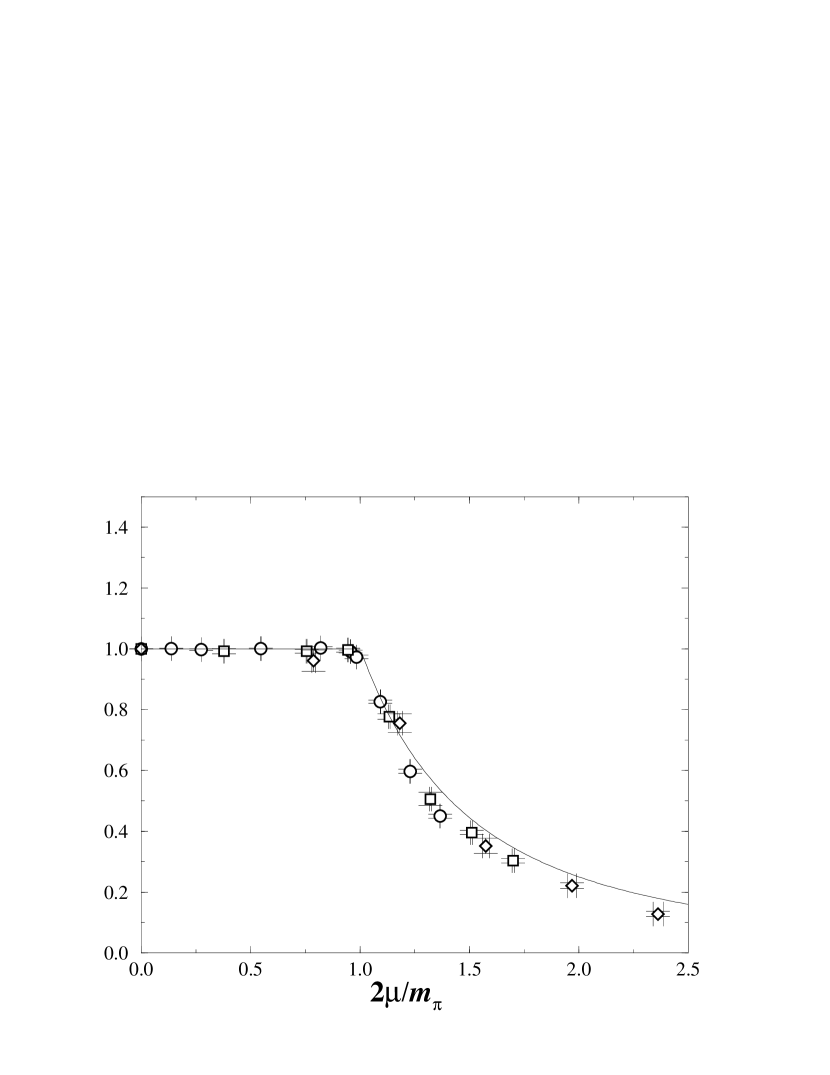
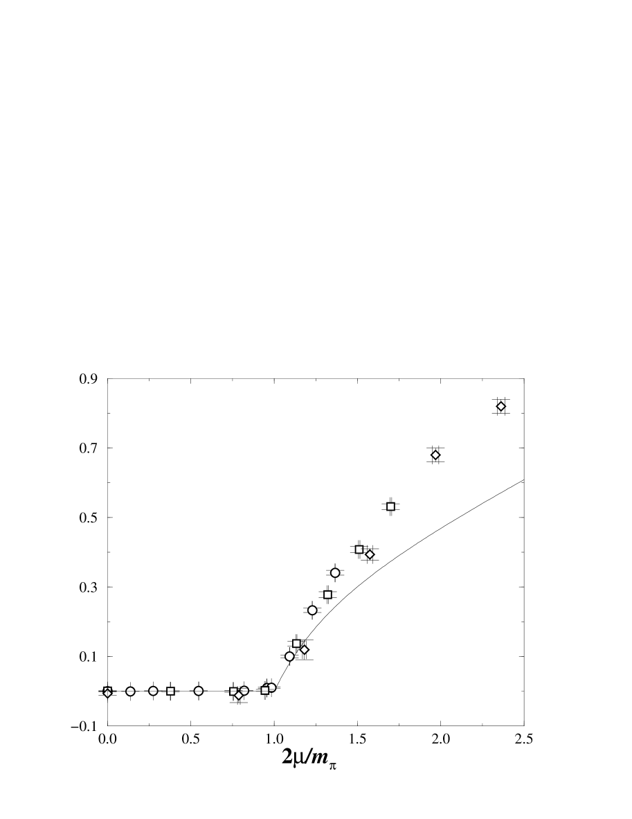
Figure 17: The scaled chiral condensate, $\langle\bar{\psi}\psi\rangle/\langle\bar{\psi}\psi\rangle_{0}$, (left) and number density, $n_{B}$, (right) together with the chiral perturbation theory prediction. (Ref. HaMoMoOeScSk)

It has been shown in Ref. HaMoMoOeScSk that the numerical data are well described by the chiral perturbation theory. Fig.17 presents the chiral condensate and the number density, respectively, together with the leading order prediction,

$$\frac{\langle\bar{\psi}\psi\rangle}{\langle\bar{\psi}\psi\rangle_{0}}=\left\{\begin{array}[]{c}1\\ \frac{1}{x^{2}}\end{array}\right.;\left(\frac{m_{\pi}}{8\langle\bar{\psi}\psi\rangle_{0}}\right)n_{B}=\left\{\begin{array}[]{cc}0&x<1\\ \frac{x}{4}(1-\frac{1}{x^{4}})&x>1\end{array}\right.$$ (67)

where

$$x\equiv\frac{2\mu}{m_{\pi}}$$ (68)

Using extended QCD inequality, Kogut, Stephanov and Toublan have shown that in SU(2) color QCD at finite density, condensation must occur in scalar diquark channel. [67] The correlator of a meson, $\bar{\psi}\Gamma\psi$ is given by $\langle\mbox{Tr}G(x,0)\Gamma G(0,x)\Gamma\rangle$, where $G=\Delta^{-1}$ are quark propagators and taken as a matrix in Dirac and color space. At $\mu=0$, Eq.(14) leads to $\Delta^{\dagger}=\gamma_{5}\Delta\gamma_{5}$. From Cauchy-Schwarz inequality, one obtains $\mbox{Tr}AB^{\dagger}\leq\sqrt{\mbox{Tr}AA^{\dagger}}\sqrt{\mbox{Tr}BB^{\dagger}}$. Then

$$\mbox{Tr}G(x,0)\Gamma G(0,x)\Gamma = \mbox{Tr}G(x,0)\Gamma\gamma_{5}G(x,0)^{\dagger}\gamma_{5}\Gamma$$ (69)

$$\leq \sqrt{G(x,0)G(x,0)^{\dagger}}\sqrt{\Gamma\gamma_{5}G(x,0)^{\dagger}\gamma_{5}\Gamma\left(\Gamma\gamma_{5}G(x,0)^{\dagger}\gamma_{5}\Gamma\right)^{\dagger}}$$

$$= \mbox{Tr}G(x,0)G(x,0)^{\dagger}$$

The right-hand side corresponds to the pion propagator which behaves as $C_{\pi}\exp(-m_{\pi}|x|)$ at large $x$. Therefore

$$Ce^{-m|x|}\leq C_{\pi}e^{-m_{\pi}|x|}$$ (70)

This relationship holds at arbitrary large $x$ only if $m\geq m_{\pi}$, i.e., the pion should be the lightest meson. This is the essence of QCD inequality.

The above QCD inequality does not hold at finite density. For SU(2), however, there is another relationship, $V\sigma_{2}G\sigma_{2}V^{-1}$, and using this the authors of Ref. KSteT show that the mass of the scalar ($0^{+},I=0$) diquark, $\psi_{C}\sigma_{2}\gamma_{5}\psi$, is lowest, where $\psi_{C}\equiv\psi^{T}C$. Therefore if diquark condensation occurs, it appears in this channel.

Table 2: Two Color

Action	parameters	comments	Ref.
Plaq. + Wilson	$N_{f}=2$, $\beta=1.4\sim 2.0$, $8^{3}\times 2$	first calculation, pseudo-Fermion Method	Nakamura84
Plaq. + KS	$\beta=1.3$, $m_{q}=0.05,0.07$, $6^{3}\times 12$	symmetries and spectrum of lattice gauge theory	HKLM99
Plaq. + KS	($\beta=1.3$, $m_{q}=0.07,0.05$), ($\beta=1.5$, $m_{q}=0.1,0.07,0.05$), ($\beta=1.3\sim 2.3$, $m_{q}=0.1$), $6^{4}$	interquark potential	MPL
Plaq. + adjoint KS	$N_{f}=4$, $\beta=2.0$, $m_{q}=0.01\sim 0.1$, $4^{3}\times 8$	adjoint dense matter, Two-Step Multi-Boson algorithm	HaMoMoOeScSk
Plaq. + KS	$N_{f}=8$, $\beta=2.0$, $m_{q}=0.025\sim 0.2$, $4^{4}$, $6^{4}$	fermion condensates	Aloisio
Plaq. + KS	$N_{f}=4$, $m_{q}=0.05$, $8^{4}$, $8^{3}\times 4$, $12^{3}\times 6$, $16^{4}$	diquark condensation, tricritical point	KTS, KTS02
Plaq. + KS	$N_{f}=4$, $\beta=1.5$, $m_{q}=0.1$, $8^{4}$, $12^{3}\times 24$	phase diagram, diquark condensation	KSHM
Plaq. + Wilson	$N_{f}=2$, $\beta=1.6$, $4^{4}$, $4^{3}\times 8$	thermodynamical quantities, Link-by-Link update	MNN1
Imp. + Wilson	$N_{f}=2,3$, $\beta=0.7$ $4^{4}$, $4^{3}\times 8,12$,	behavior of hadrons, Link-by-Link update	MNN2
Plaq. + KS fermions	Nf=8, $12\times 12\times 24\times 4$, $\beta=1.1$, $m_{q}$=0.05, 0.07, 0.1	chiral condensation	LMNT

4.1 Diquark condensation – Super fluidity

Figure 18: Wilson line and condensate vs. $\beta$ calculated by Kogut, Toublan and Sinclair. Standard gauge + Staggered fermions. $N_{F}=4$. Left : $\mu=0.0$ Right : $\mu=0.3$. (Ref. KTS02)

In Figs.18, we show the Wilson line, the chiral condensate $\langle\bar{\chi}\chi\rangle$ and the diquark condensate $\langle\chi\sigma_{2}\chi\rangle$ obtained by Kogut, Toublan and Sinclair. [63] Here $\chi$ and $\bar{\chi}$ are staggered fermions. Using the staggered fermions, they simulated a system with a diquark source,

$$S=\bar{\chi}\Delta\chi+j\bar{\chi}\sigma_{2}\bar{\chi}^{T}+j^{*}\chi^{T}\sigma_{2}\chi+S_{G}=(\chi,\chi^{T})\left(\begin{array}[]{cc}j\sigma_{2}&\frac{1}{2}\Delta\\ -\frac{1}{2}\Delta^{T}&j^{*}\sigma_{2}\end{array}\right)\left(\begin{array}[]{c}\bar{\chi}^{T}\\ \chi\end{array}\right)+S_{G}$$ (71)

After integrating out $\bar{\chi}$ and $\chi$, we obtain

$$Z=\int\mathcal{D}U\sqrt{\det\Delta\Delta^{T}+|j|^{2}}\,e^{-\beta S_{G}}.$$ (72)

The fermionic measure is always positive. The source term acts as an external field in spin systems, and $j$ should be extrapolated to zero at the end. Due to the square root, one cannot employ Hybrid Monte Carlo simulation, but the molecular-dynamics type algorithm is available to generate configurations.

Fig.18 (right) indicates the temperature behavior of the phase at fixed finite $\mu$ with small $j$. When the temperature increases (the coupling increases), the Wilson line and the chiral condensate increase, which shows the confinement to deconfinement transition. The same behavior is seen at zero chemical potential shown in Fig.18 (left). A remarkable feature at finite $\mu$ is that $\langle\chi^{T}\sigma_{2}\chi\rangle$ has finite values at low temperature. Therefore at finite density and low temperature, there is a region in which the di-quark condensation occurs. From these observations, they suggest the phase shown in Fig.19.

The operator $\langle\chi^{T}\sigma_{2}\chi\rangle$ is a color singlet and cannot bring about color charge. Therefore this is not a color super conductivity, but it can be super fluidity such as liquid ${}^{3}{\rm H}e$. This region belongs to the confinement phase, and this is probably because this diquark condensation phase is revealed by the color singlet external source.

Figure 19: Schematic phase diagram in the $(T,\mu)$ plane by Kogut, Toublan and Sinclair. (Ref. KTS02)

4.2 Hadrons at finite density – In-medium effect ?

In-medium hadron features are of great interest in high-energy phenomenology. Brown and Rho conjectured that

$$\frac{m^{*}}{m}=\frac{f_{\pi}^{*}}{f_{\pi}},$$ (73)

which is now known as Brown Rho scaling, to explain the large low mass lepton pair enhancement observed in CERES [15]. Here $m^{*}$ and $f_{\pi}^{*}$ are the mass and the pion decay constant in the medium [70]. Based on the QCD sum rule, Hatsuda and Lee predicted a decrease of $\rho$ meson mass as a function of $\mu$ [71]. Harada et al. showed that the vector meson mass vanishes at the critical density as a consequence of an effective theory with hidden local symmetry [72]. Yokokawa et al. proposed simultaneous softening of $\sigma$ and $\rho$ mesons associated with the chiral restoration [73]. If lattice data show such a phenomenon, it is a new feature of QCD at finite density, and will become an interesting experimental target in future heavy ion experiments.

Recently, Muroya, Nakamura and Nonaka reported a strange behavior of the propagator of a vector meson channel with chemical potential [74]. They investigated finite density state of color SU(2) QCD with Wilson fermion. As for the gauge part of the lattice action, both plaquette and Iwasaki improved actions are adopted. In order to make a reliable update, the ratio of fermion determinants is calculated exactly through the Woodbury formula. As a result, the lattice is limited to a small size. They investigated the propagators of mesons and diquarks; pseudo-scalar ($\pi$), scalar ($a_{0}$), vector ($\rho$) mesons, and scalar diquark ($q\gamma_{5}q$), pseudo-scalar diquark ($q1q$) and axial-vector diquark ($q\gamma_{\mu}q$) are studied. At $\mu=0$, the propagators of the corresponding meson and diquark are degenerate with each other. With finite $\mu$, the propagators change their shapes. It is quite different from the finite temperature case, the propagator of the pseudo-scalar meson changes only slightly and the vector meson becomes lighter. The propagators of the corresponding diquarks show clear asymmetry in the chronological direction due to the charge corresponding to the chemical potential. However, the behavior of the obtained mass is very mild. Only the vector meson mass shows a marked change around $\mu a=0.7$. This behavior might be the expected result of the phenomenological models. Figs.20 are typical behaviors of masses of the pseudo-scalar, vector mesons, and di-quarks as a function of $mu$.

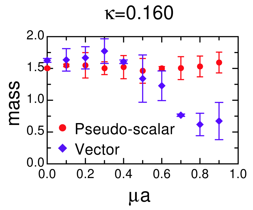
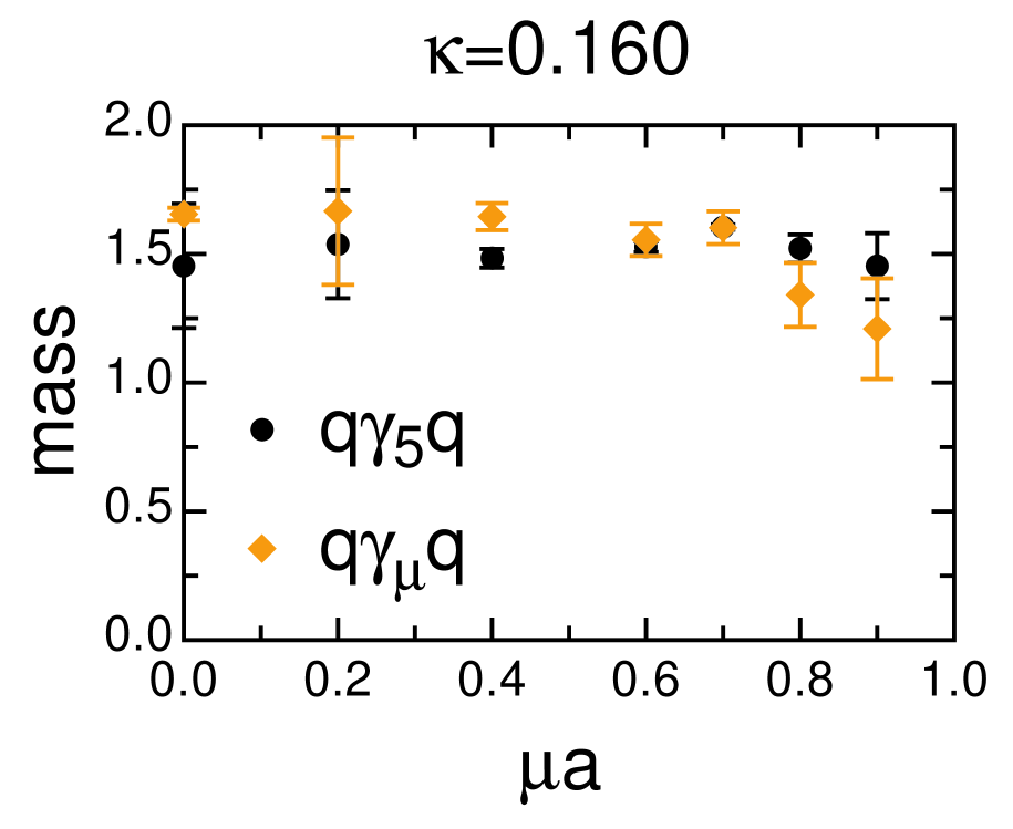
Figure 20: Pseudo scalar and vector meson masses (left) and corresponding di-quark (baryon) masses (right). (Ref. MNN03).

The propagators of the scalar meson and pseudo scalar diquark decay so quickly that it is very difficult to catch signal against noise.

Another possible explanation for the lightening of the mass of the mesonic channel is a particle-hole pair around a Fermi surface. Hands, Kogut, Strouthos and Tran investigated the (2+1)-dimensional Gross-Neveu mode and discussed the effect of the Fermi surface. They evaluate the mesonic propagator in the high density state with a Fermi surface. In the mesonic channel, in addition to the ordinary quark-anti-quark pair which contributes as a massive meson, quark-hole gapless pair around Fermi surface may exist. In Ref.[75], authors investigated propagators with fixed momenta and found that at high density, a mesonic propagator whose momentum is up to some value shows massless behavior. On the other hand, propagators with larger momenta behave massive. The existence of such a particle-hole pair is well known in the many-body theory and from direct results of the Fermi surface. In Ref.[75], a momentum dependent massless mode appears in the scalar channel and vector channel, but, in Ref. MNN03 it appears in the vector channel only. In order to clarify the Fermi surface effect, we need larger lattice simulation and calculation of the $\sigma$ channel which also contains a disconnected diagram.

5 Related works

5.1 Gross-Neveu model - Simple model for test

QCD in four dimensions is highly nontrivial. A simple model may help us to understand the theory, and may give us a hint toward determining a correct route. The Gross-Neveu model has been studied for this purpose.

Let us start from a model in two dimensions with Nambu-Jona-Lasinio type four fermion interaction which has a ‘flavor’ degree of freedom $N$. The action is given by

$$S=\sum_{k=1}^{N}\left[\bar{\psi}^{(k)}(\gamma_{\mu}\partial_{\mu}+m)\psi^{(k)}-\frac{g^{2}}{2N}\{(\bar{\psi}^{(k)}\psi^{(k)})^{2}+(\bar{\psi}^{(k)}i\gamma_{5}\psi^{(k)})^{2}\}\right],$$ (74)

where the Dirac matrices are

$$\gamma_{1}=\sigma_{2},\gamma_{2}=\sigma_{1},\gamma_{5}=i\gamma_{1}\gamma_{2}=\sigma_{3}.$$ (75)

When its mass $m$ vanishes, Eq.(74) possesses the chiral symmetry,

$$\psi\rightarrow e^{i\gamma_{5}\theta}\psi,\bar{\psi}\rightarrow\bar{\psi}e^{i\gamma_{5}\theta}.$$ (76)

We introduce two auxiliary fields, $\sigma(x)$ and $\pi(x)$, which correspond to $-(g^{2}/N)\bar{\psi}\psi$ and $-(g^{2}/N)\bar{\psi}i\gamma_{5}\psi$, respectively, in the standard manner,

$$S = \bar{\psi}(\gamma_{\mu}\partial_{\mu}+m)\psi-\frac{g^{2}}{2N}\{(\bar{\psi}\psi)^{2}+(\bar{\psi}i\gamma_{5}\psi)^{2}\}$$ (77)

$$+\frac{N}{2g^{2}}(\sigma+\frac{g^{2}}{N}\bar{\psi}\psi)^{2}+\frac{N}{2g^{2}}(\pi+\frac{g^{2}}{N}\bar{\psi}i\gamma_{5}\psi)^{2},$$

$$= \bar{\psi}(\gamma_{\mu}\partial_{\mu}+m+\sigma+i\gamma_{5}\pi)\psi+\frac{N}{2g^{2}}(\sigma^{2}+\pi^{2}).$$

Here we suppress the flavor index $k$. It is easy to verify that Eq.(77) is invariant under the following rotation together with Eq.(76) in a massless limit,

$$\left(\begin{array}[]{c}\sigma\\ \pi\end{array}\right)\rightarrow\left(\begin{array}[]{cc}\cos 2\theta&\sin 2\theta\\ -\sin 2\theta&\cos 2\theta\end{array}\right)\left(\begin{array}[]{c}\sigma\\ \pi\end{array}\right)$$ (78)

In a large $N$ limit, the fields $\sigma$ and $\pi$ can be replaced by their mean fields, and we may rotate them so that $\pi=0$. Then we have a model with only the first four-fermion interaction term in Eq.(74), or

$$S=\bar{\psi}(\gamma_{\mu}\partial_{\mu}+\sigma)\psi+\frac{N}{2g^{2}}\sigma^{2}.$$ (79)

Although the model has no confinement, it has the following features common to QCD:

• it is an asymptotically free theory,

• it shows spontaneous breakdown of a (discrete) chiral symmetry, i.e., $\psi\rightarrow\gamma_{5}\psi$.

The Gross-Neveu model is well studied in the continuum,

• the phase structure at finite temperature and density is obtained in $N\rightarrow\infty$ limit by a mean field approach.

• Finite $N$ case can be treated by the factorized S-matrix method [78].

• There is a conjecture that a generalization of the Gross-Neveu model from $U(N)$ to $O(N)$ flavor symmetry leads to the appearance of a pairing condensate at high density. [79]

There are two lattice studies of the Gross-Neveu model in the literature. Karsch, Kogut and Wyld analysed the staggered fermion version of Eq.(77) [82],

$$S=\sum_{k=1}^{N}\bar{\chi}^{k}\Delta\chi^{k}+\frac{1}{2g^{2}}\sigma^{2},$$ (80)

where the fermion matrix is given by

$$\Delta_{ij}=\frac{1}{4}(\sigma_{j}+\sigma_{j-\hat{0}}+\sigma_{j-\hat{1}}+\sigma_{j-\hat{0}-\hat{1}})\delta_{ij}+\frac{1}{2}(e^{\mu}\delta_{j,i+\hat{0}}-e^{-\mu}\delta_{j,i-\hat{0}})+\frac{1}{2}(-1)^{t}(\delta_{j,i+\hat{1}}-\delta_{j,i-\hat{1}})$$ (81)

All elements of the fermion matrix are real, therefore its determinant is also real. In Ref. GN-lat1, the Langevin algorithm was used to simulate the system with $N=12$. Fig.21 shows typical simulation results.

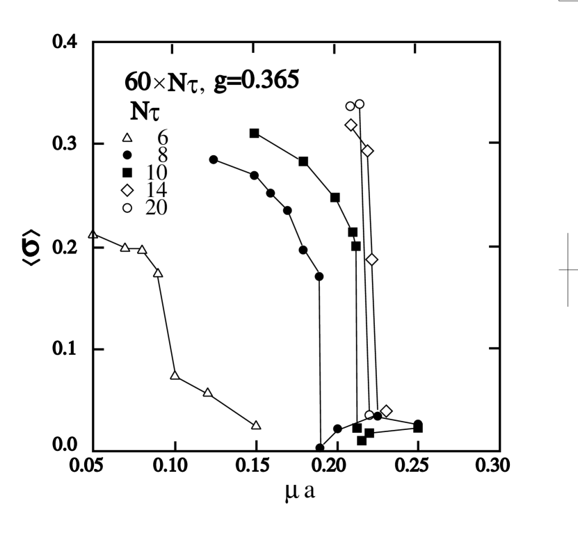
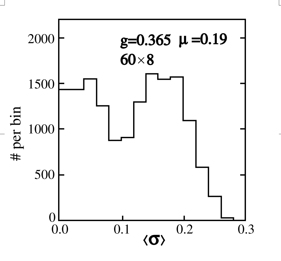
Figure 21: Left : $\langle\sigma\rangle$ as a function of $\mu$ on lattices of size $60\times N_{\tau}$,$N_{\tau}=6,8,10,14,20$. Right : Coexisting states at $\mu_{c}$. Ref.GN-lat1.

Izubuchi, Noaki and Ukawa investigated a lattice version of Eq.74 using Wilson fermions at finite temperature and density, [83]

$$S= - \frac{1}{2a}[\bar{\psi}(x)(r-\gamma_{1})\psi(x+\hat{1})\bar{\psi}(x)(r+\gamma_{1})\psi(x-\hat{1})]$$ (82)

$$- \frac{1}{2a}[\bar{\psi}(x)(r-\gamma_{2})e^{-\mu a}\psi(x+\hat{2})\bar{\psi}(x)(r+\gamma_{1})e^{\mu a}\psi(x-\hat{1})]$$

$$+ \frac{1}{a}(2r+\delta m)\bar{\psi}(x)\psi(x)-\frac{g_{\sigma}^{2}}{2N}(\bar{\psi}(x)\psi(x))^{2}-\frac{g_{\pi}^{2}}{2N}(\bar{\psi}(x)i\gamma_{5}\psi(x))^{2}.$$

Here they introduce two couplings $g_{\sigma}$ and $g_{\pi}$ to controle the continuum limit. The lattice effective potential is constructed with two auxiliary fields, $\sigma$ and $\pi$ as in the continuum,

$$V_{L}=-\left(\frac{\delta m_{L}}{g_{\sigma}^{2}}+2C_{1}\right)\sigma_{L}+\left(\frac{1}{g_{\pi}^{2}}-2C_{0}\right)\pi_{L}^{2}+\left(\frac{1}{g_{\sigma}^{2}}-C_{0}+2C_{2}\right)\sigma_{L}^{2}$$

$$+\frac{1}{4\pi}(\sigma_{L}^{2}+\pi_{L}^{2})\log\frac{\sigma_{L}^{2}+\pi_{L}^{2}}{e}+O(a^{3}),$$ (83)

where $C_{0}$, $C_{1}$ and $C_{2}$ are constant. In order to get the correct chiral symmetric theory in the continuum, we tune three parameters, $g_{\pi}$, $g_{\sigma}$ and $\delta m_{L}$ so that

$$\frac{1}{g_{\pi}^{2}}=\frac{1}{g_{\sigma}^{2}}+4C_{2}+O(a),$$

$$\frac{\delta m_{L}}{g_{\sigma}^{2}}=-2C_{1}+O(a^{2}).$$ (84)

5.2 NJL model

At present, there are no reliable methods for evaluating low temperature and high density regions in nonperturbative QCD calculation. Therefore effective theories such as Nambu-Jona-Lashino (NJL) model play an important role and the comparison of the results of lattice QCD for a simple case to the results of effective theories is a meaningful approach in order to understand the superconducting behavior at high density. Hands and Walters apply the lattice analyses to the NJL model in (3+1)-dimension, focusing on BCS diquark condensation.[84] The action of this model is written by

$$S=\psi^{\rm{tr}}{\cal{A}}\psi+\frac{2}{g^{2}}\sum_{\tilde{x}}(\sigma^{2}+\vec{\pi}\cdot\vec{\pi}),$$ (85)

where the bispinor $\psi$ is written in terms of staggered isospinor fermions fields, $\psi^{\rm{tr}}=(\bar{\chi},\chi^{\rm{tr}})$ and $\sigma$ and the triplet $\vec{\pi}$ are real auxiliary fields defined on the dual site $x$. In the fermion matrix ${\cal{A}}$ they introduce the diquark source term $j$,

$${\cal{A}}=\frac{1}{2}\left(\begin{array}[]{cc}\bar{j}\tau_{2}&M\\ M^{\rm{tr}}&j\tau_{2}\end{array}\right),$$ (86)

where the matrix $M$ is defined by

$$M^{pq}_{xy}[\sigma,\vec{\pi}] = \frac{1}{2}\delta^{pq}\left[({\rm e}^{\mu}\delta_{yx+\hat{0}}-{\rm e}^{-\mu}\delta_{yx-\hat{0}})\right.$$ (87)

$$+\sum_{\nu=1,2}\eta_{\nu}(x)(\delta_{yx+\hat{\nu}}-\delta_{yx-\hat{\nu}})+2m_{0}\delta_{xy}\left.\right]$$

$$+\frac{1}{16}\delta{xy}\sum_{\langle\tilde{x},x\rangle}(\sigma(\tilde{x})\delta^{pq}+i\epsilon(x)\vec{\pi}(\tilde{x})\cdot\vec{\tau}^{pq}).$$

Here $m_{0}$ is the bare mass and $\eta_{\nu}(x)$, $\epsilon(x)$ are the phases $(-1)^{x_{0}+\cdots x_{\nu-1}}$ and $(-1)^{x_{0}+x_{1}+x_{2}+x_{3}}$, respectively. The $\vec{\tau}$ are Pauli matrices and $\langle\tilde{x},x\rangle$ represents the set of 16 dual lattice sites neighboring $x$.

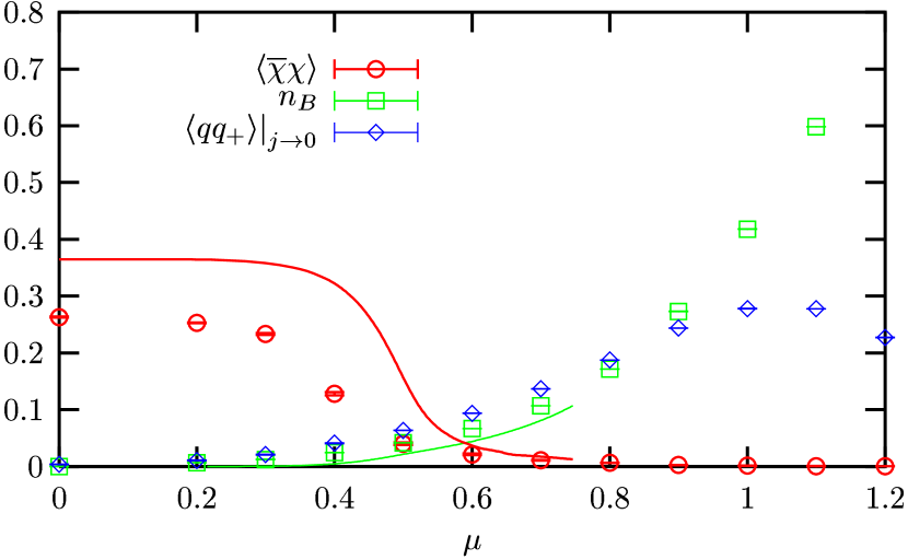
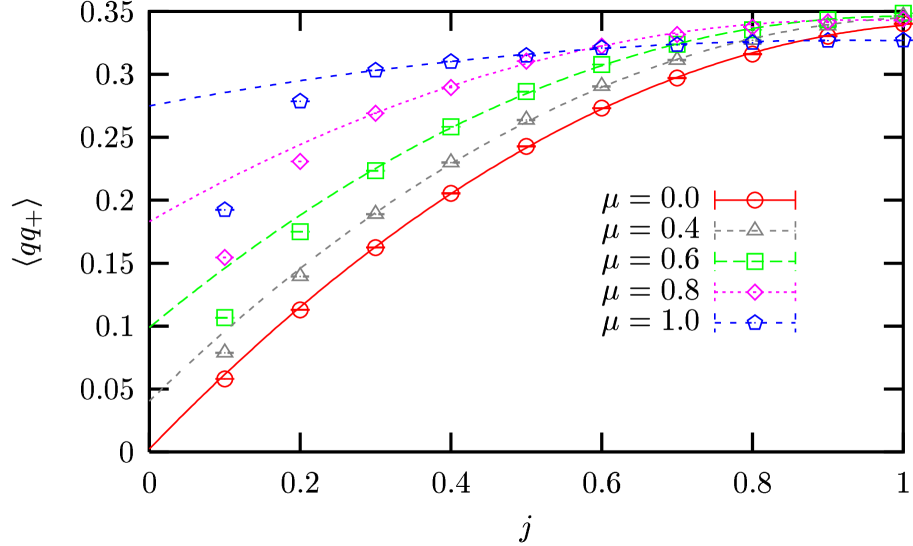
Figure 22: The diquark condensate, $\langle qq\rangle$ as a function of $\mu$(left). $\langle qq\rangle$ as a function of $j$ (right).

They measure diquark condensate $\langle qq\rangle$ as a function of chemical potential, extrapolating to $j\rightarrow 0$. From this analysis, they determine the existence of a nonzero BCS condensate at high baryon density (Fig. 22 (left)) . However, the behavior of $\langle qq\rangle$ as a function of $\mu$ depends on the evaluation of the data at $j\rightarrow 0$. They ignore the values of $\langle qq\rangle$ at small $j$, because at high $\mu$, $\langle qq\rangle$ at small $j$ falls rapidly away from the tendency of $\langle qq\rangle$ at large $j$ (Fig. 22(right)). They discuss that the low-$j$ discrepancy comes from the finite volume effect and the partially quenched approximation and some issues concerning thermodynamic limit need to be resolved for a definite conclusion.

5.3 Strong coupling calculation

It is comfortable if we have any analytical or semi-analytical method to study QCD at finite baryon density in non-perturbative region. Strong coupling approximation of lattice QCD is one of such possibilities. Indeed the lattice formulation was introduced to allow the strong coupling expansion and the confinement was shown there. We can also compare our numerical data to the analytical calculations and take a deep view of lattice results.

When the gauge coupling $g$ is very large, $\beta S_{G}=6/g^{2}S_{G}$ may drop,

$$Z=\int\mathcal{D}U\mathcal{D}\bar{\psi}\mathcal{D}\psi\,e^{-\bar{\psi}\Delta\psi}.$$ (88)

In this case, the integrations over time like link variables, $U_{4}(x)$, and space-like ones, $U_{i}(x)$, are decouples, and one can integrate over the gauge fields.

The first strong coupling calculation was performed by Ilgenfritz and Kripfganz [86] and Damgaard, Hochberg and Kawamoto, [87] together with the mean field approximation. Bilić, Demeterfi and Petersson extended the calculation to the next order of $1/g^{2}$. [88] Recently Nishida, Fukushima and Hatsuda applied the strong coupling method to two-color QCD to study the dynamics of the theory. [89]

For warming-up, let us first study a very simple case in a pedagogical way:

$$Z=\int dUd\bar{\psi_{1}}d\psi_{1}d\bar{\psi_{2}}d\psi_{2}e^{\bar{\psi}_{1}U\psi_{2}-\bar{\psi}_{2}U^{\dagger}\psi_{1}},$$ (89)

i.e., two fermion fields, $\psi_{1}^{a},\psi_{2}^{a}$ are connected by a link filed $U$, where $a=1,2,\cdots,N_{c}$ are color index. Series expansion of the exponential is finie due to the nil potency of the Grassmann variable. With the help of group integration properties,

$$\int dU = 1$$

$$\int dUU_{a,b}{U^{\dagger}}_{c,d}=\frac{1}{3}\delta_{a,d}\delta_{b,c}=\mbox{ \includegraphics[width=62.59596pt,height=56.9055pt,keepaspectratio]{meson-line.eps} }$$

$$\int dUU_{a_{1},b_{1}}U_{a_{2},b_{2}}U_{a_{3},b_{3}} = \frac{1}{3!}\epsilon_{a_{1}a_{2}a_{3}}\epsilon_{b_{1}b_{2}b_{3}}=\mbox{ \includegraphics[width=62.59596pt,height=56.9055pt,keepaspectratio]{baryon-line.eps} }$$

$$\int dU{U^{\dagger}}_{a_{1},b_{1}}{U^{\dagger}}_{a_{2},b_{2}}{U^{\dagger}}_{a_{3},b_{3}} = \frac{1}{3!}\epsilon_{a_{1}a_{2}a_{3}}\epsilon_{b_{1}b_{2}b_{3}}$$ (90)

where $U_{a,b}$ is $(a,b)$ element of the matrix $U$, we obtain

$$Z = 1+\frac{1}{3}M_{1}M_{2}+(-\bar{B}_{1}B_{2}+\bar{B}_{2}B_{1})+\cdots$$ (91)

$$\sim e^{\frac{1}{3}M_{1}M_{2}+(-\bar{B}_{1}B_{2}+\bar{B}_{2}B_{1})},$$

where

$$M_{i} \equiv {\bar{\psi}_{i}}^{a}{\psi_{i}}^{a},$$

$$B_{i} \equiv \frac{1}{3!}\epsilon_{a_{1}a_{2}a_{3}}{\psi_{i}}^{a_{1}}{\psi_{i}}^{a_{2}}{\psi_{i}}^{a_{3}}.$$ (92)

More systematic and precise formulae are given in Ref.[90]. Using the identities with auxiliary bosonic field $\phi$ and fermionic field $b$,

$$e^{\frac{1}{2}^{t}{M}\mathcal{V}^{-1}{M}}=\int d\phi_{1}d\phi_{2}\,e^{-\frac{1}{2}^{t}{\phi}\mathcal{V}{\phi}-^{t}{\phi}{M}},$$ (93)

$$e^{\bar{B}\mathcal{W}^{-1}B}=\int d\bar{b}db\,e^{-\bar{b}\mathcal{W}b+\bar{b}B+\bar{B}b},$$ (94)

we linearize $M$ and $B$ fields, where $M=^{t}(M_{1}M_{2})$.

Now we come back to the realistic case. We integrate first the spatial link variables for the staggered fermions,

$$Z=\int\mathcal{D}U_{4}\mathcal{D}\bar{\chi}\mathcal{D}\chi\exp\left\{-\sum_{x,y}\bar{\chi}(x)\left[m\delta_{x,y}+\frac{1}{2r}e^{\mu r}U_{4}(x)\delta_{x,y-\hat{4}}\right.\right.$$

$$\left.-\frac{1}{2r}e^{-\mu r}U_{4}(x)^{\dagger}\delta_{x,y+\hat{4}}\right]\chi(y)-\frac{1}{4N_{c}}\sum_{\langle x,y\rangle}\bar{\chi}(x)\chi(x)\bar{\chi}(y)\chi(y)$$

$$\left.-\frac{1}{32N_{c}^{2}(N_{c}-1)}\sum_{\langle x,y\rangle}[\bar{\chi}(x)\chi(x)]^{2}[\bar{\chi}(y)\chi(y)]^{2}\right\}$$ (95)

where an anisotropy parameter of time-like and space-like lattice spacing, $r\equiv a_{t}/a_{s}$, is introduced to controle the temperature. Introducing auxiliary fields, $\lambda$, we can linearize the exponential,

$$Z=\int\mathcal{D}U_{4}\mathcal{D}\bar{\chi}\mathcal{D}\chi\mathcal{D}\lambda\exp\left\{-\frac{N_{c}}{d}\sum_{x,y}(\lambda(x)-m)V^{-1}(x,y)(\lambda(y)-m)\right.$$

$$\left.-\sum_{x,y}\bar{\chi}(x)\left[\lambda(x)\delta_{x,y}+\frac{1}{2r}e^{\mu r}U_{4}(x)\delta_{x,y-\hat{4}}-\frac{1}{2r}e^{-\mu r}U_{4}(x)^{\dagger}\delta_{x,y+\hat{4}}\right]\chi(y)\right\}$$ (96)

where $d$ is the spatial dimension ($=3$), and the matrix $V(x,y)$ is defined by

$$V(x,y)=\frac{1}{2d}\sum_{k=1}^{d}(\delta_{y,x+\hat{k}}+\delta_{y,x-\hat{k}})$$ (97)

The integration over $\bar{\chi}$ and $\chi$ can be performed. Then we can further integrate over $U_{4}$. When $\lambda$ is constant (mean field approximation), then

$$Z=2\cosh(N_{t}N_{c}\mu r)+\frac{\sinh(N_{c}+1)N_{t}\lambda^{\prime}}{\sinh(N_{t}\lambda^{\prime})}$$ (98)

where $\lambda^{\prime}=\sinh^{-1}[(\lambda+m)r]$. $\lambda$ is determined by minimizing the free energy $F=N_{t}N_{c}\lambda^{2}/d-\log Z$, i.e., $\partial F/\partial\lambda=0$. The chiral condensation is given by the $\lambda$ by $\langle\bar{\chi}\chi\rangle=2N_{c}\lambda/d$. In the infinite coupling limit, the transition value of the chemical potential is given as

$$\mu_{0}=\frac{1}{r}\sinh^{-1}(\lambda_{0}r)-\frac{\lambda^{2}_{0}}{dr},$$ (99)

where

$$\lambda_{0}=\frac{1}{r\sqrt{2}}(\sqrt{1+d^{2}r^{4}}-1)^{1/2}.$$ (100)

The transition point with $1/g^{2}$ correction can be found in Ref.[88].

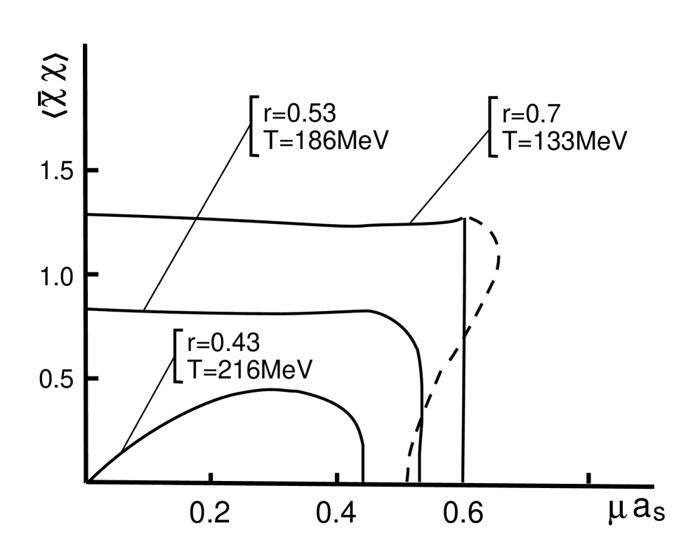
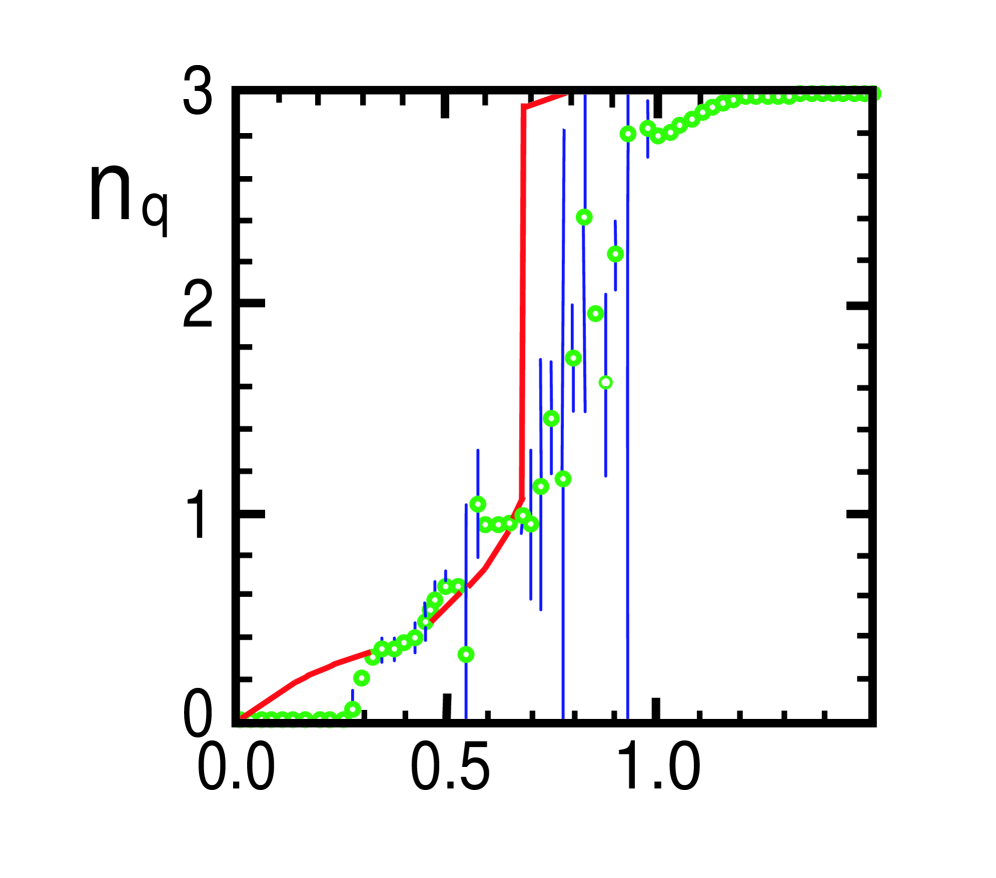
Figure 23: Strong coupling calculations by Bilić, Demeterfi and Petersson (Ref. BDP). Chiral condensate as a function of $\mu$ for various temperatures at $6/g^{2}=2$. The dashed line represents the instability region. (left) Comparison of the strong coupling calculation of the quark number density with numerical data for $N_{t}=4$ and $6/g^{2}=4.8$. The points are data of Ref.[37]. (right)

In Fig.23, we show the chiral condensate as a function of the chemical potential for various temperatures at $6/g^{2}=2$ taken from Ref.[88] where the $1/g^{2}$ correction is included. They calculated also the quark number density as a function of the chemical potential and found good agreement with the numerical calculation given by Hasenfratz and Toussaint [37].

Karsch and Mütter have given an elegant form, ‘monomer-dimer-polymer’ system. [91] For the fermion matrix of the form,

$$\Delta=2ma+\sum_{\langle xy\rangle}U(x,y)\zeta(x,y),$$ (101)

$$Z=\int\mathcal{D}\bar{\psi}\mathcal{D}\psi\,e^{2ma\sum_{x}M(x)}\Pi_{\langle xy\rangle}F(x,y).$$ (102)

where

$$F(x,y) = \int\mathcal{D}U\,e^{\bar{\psi}(x)U\zeta(x,y)\psi(y)+\bar{\psi}(y)U^{\dagger}\zeta(y,x)\psi(x)}$$ (103)

$$= 1-\frac{1}{3}\rho(x,y)M(x)M(y)+\frac{1}{12}(\rho(x,y)M(x)M(y))^{2}-\frac{1}{36}(\rho(x,y)M(x)M(y))^{3}$$

$$+\zeta(x,y)^{3}\bar{B}(x)B(y)+\zeta(y,x)^{3}\bar{B}(y)B(x).$$

Here $M(x)$, $B(x)$ and $\bar{B}(x)$ are ‘meson’, ‘baryon’ and ‘antibaryon’ fields. For staggered fermions, the quark field $\psi(x)$ has only color degrees of freedom, not Dirac indices. Meson, baryon and antibaryon fields are given as,

$$M(x)\equiv\bar{\psi}(x)\psi(x)=\sum_{a=1,2,3}\bar{\psi}^{a}(x)\psi^{a}(x)=\sum_{a=1,2,3}M_{a}(x),$$ (104)

$$B(x) \equiv \psi^{1}(x)\psi^{2}(x)\psi^{3}(x),$$

$$\bar{B}(x) \equiv \bar{\psi}^{3}(x)\bar{\psi}^{2}(x)\bar{\psi}^{1}(x),$$ (105)

respectively, and

$$e^{2maM(x)}=1 + 2ma\left(M_{1}(x)+M_{2}(x)+M_{3}(x)\right)$$ (106)

$$+ (2ma)^{2}\left(M_{1}(x)M_{2}(x)+M_{2}(x)M_{3}(x)+M_{3}(x)M_{1}(x)\right)$$

$$+ (2ma)^{3}\left(M_{1}(x)M_{2}(x)M_{3}(x)\right).$$

The last equation gives ‘monomer’ contributions. $\rho(x,y)$ is the ‘mesonic’ link factor,

$$\rho(x,y)=\zeta(x,y)\zeta(y,x),$$ (107)

from which three types of “dimers”, $\rho(x,y)$, $\rho(x,y)^{2}$ and $\rho(x,y)^{3}$, are constructed. For staggered fermions,

$$\zeta(x,y)=\eta(x,y)\left\{\begin{array}[]{ll}\pm\frac{a_{s}}{a_{t}}\,e^{\pm\mu a_{t}},&\mbox{for }x=y+\hat{4},\\ \pm 1,&\mbox{for }x=y+\hat{k},(k=1,2,3)\end{array}\right.$$ (108)

with $\eta$ being the staggered sign factor.

Integration over Grassmann variables, $\psi$ and $\bar{\psi}$, is straightforward. Nonvanishing contributions appear only if each site of the lattice is occupied either by three mesons, $M_{1}(x)M_{2}(x)M_{3}(x)$ or by a baryon-antibaryon pair, $\bar{B}(x)B(x)$. Finally, the partition function is written as a sum over monomer-dimer loop configurations $K$,

$$Z(2ma,a_{s}/a_{t},\mu a_{t})=\sum_{K}w_{K},$$ (109)

where

$$w_{K} = (2ma)^{(\mbox{\# of Monomer})}\left(\frac{a_{s}}{a_{t}}\right)^{2(\mbox{\# of Dimer lines in t direction})}$$ (110)

$$\times \left(\frac{1}{3}\right)^{(\mbox{\# of the first and second type Dimers})}\Pi_{x}w(x)\Pi_{C}w(C).$$

$w(x)$ and $w(C)$ are site and loop weights associated with the configuration.

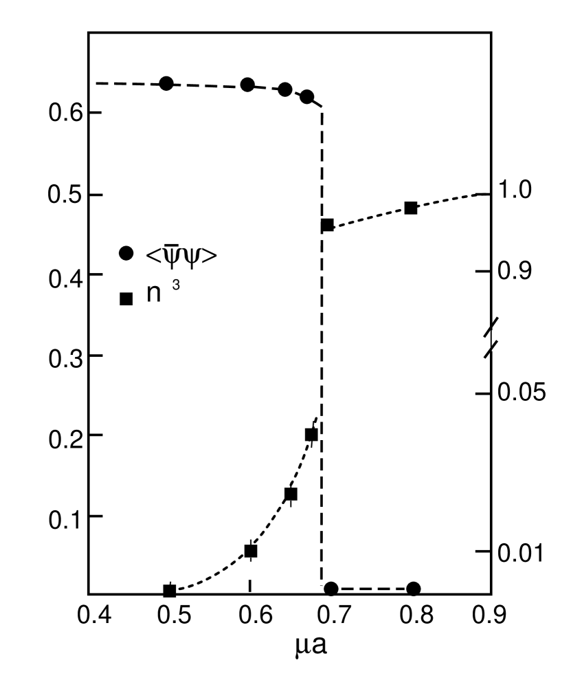
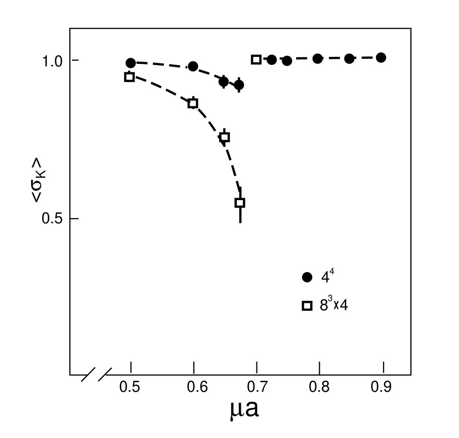
Figure 24: (a) The chiral condensate $\langle\bar{\psi}\psi\rangle=V^{-1}\partial logZ/\partial(2ma)$ and baryon number density $na^{3}=(3VN_{t})^{-1}\partial logZ/\partial(\mu a_{t})$. (b) The average sign of the Boltzmann weights. (Ref. KaMu89)

In Eq.(110), $w_{K}$ is not always positive. A sign $\sigma_{K}$ for each monomer-dimer loop configuration is introduced as

$$w_{K}=\sigma_{K}|w_{K}|,$$ (111)

and the simulation was carried out with the positive Boltzmann weight $|w_{K}|$,

$$\langle O\rangle=\frac{\langle\sigma_{K}O\rangle_{+}}{\langle\sigma_{K}\rangle_{+}}.$$ (112)

Fig.24 shows the chiral condensate and baryon number density as a function of $\mu a$ for $ma=0.1$ on $8^{3}\times 4$ lattice obtained by Karsch and Mütter. They determined that $\mu_{c}a=0.69\pm 0.015$. The average of the sign factor drops at the critical $\mu$ shown in Fig.24-(b).

5.4 Canonical ensemble

A thermodynamical system can be studied either as a grand canonical formulation or as a canonical one. When the grand canonical partition function $Z(\mu)$ is expanded in terms of the fugacity, $\zeta\equiv\exp(\mu/T)$, each coefficient is a canonical partition function $Z_{N}$ with a fixed quark baryon number $N$,

$$Z(\mu/T)=\sum_{N=-\infty}^{+\infty}\left(e^{\frac{\mu}{T}}\right)^{N}Z_{N}.$$ (113)

The canonical partition function can be formally obtained from the grand canonical partition function with imaginary chemical potential, [58, 96]

$$Z_{N}=\frac{1}{2\pi}\int_{0}^{2\pi}d\phi Z(i\phi\equiv\mu/T)=\sum_{n,\bar{n}}C(n,\bar{n})\zeta^{n}\zeta^{*\bar{n}},$$ (114)

where $\zeta=e^{i\phi},\zeta^{*}=e^{-i\phi}$. The canonical partition function with the quark baryon number $N=n-\bar{n}$ has contributions from $\zeta^{n}\zeta^{*\bar{n}}$ terms in the grand partition function. Miller and Redlich developed a general lattice canonical formulation, and investigated it using the hopping parameter expansion.

To date, only one numerical simulation was performed by Engels et al. [97] They used Wilson fermions, Eq.(18), and the expression (28). Then the coefficient of $\zeta^{n}\zeta^{*\bar{n}}$ should include $\kappa^{n+\bar{n}}$. Therefore for a heavy quark system, i.e., for small $\kappa$, the leading contribution comes from the $\bar{n}=0$ sector. An explicit expression of the expansion is very complicated, and yet they succeeded in calculating up to $N=12$ in the quenched approximation. The baryon number density is given as

$$n_{B}=\frac{B/3}{N_{s}a^{3}}.$$ (115)

$N=12$ on $8^{3}\times 2$ lattice at $T\sim T_{c}=270$ MeV corresponds to $n_{B}\sim 0.15$ fm^-3 , i.e., approximately nuclear matter density.

The heavy quark potential shows finite values for the large distance shown in Fig.25. $N=6$ on this lattice at $T\sim 0.86$ $T_{c}$ corresponds to $n_{B}=0.049$ fm^-3. The heavy quark potential is screened even below the nuclear matter density.

Figure 25: Heavy quark potential for $T\simeq 0.86T_{c}$ and $B=0$ and 6. on $16^{3}\times 4$.

5.5 Density of states method

In lattice QCD, the average value of an operator $\langle O\rangle$ is given by

$$\langle O\rangle=\frac{1}{Z}\int\mathcal{D}UO[U]\det\Delta(U)e^{-\beta S_{g}(U)},$$ (116)

with

$$Z=\int\mathcal{D}U\det\Delta(U)e^{-\beta S_{g}(U)}.$$ (117)

It is impractical to directly perform this integration of very high dimensions. Instead, we can use a importance sampling where configurations $U_{i}$ are generated with the probability distribution:

$$P(U)\propto\det\Delta(U)e^{-\beta S_{g}(U)}$$ (118)

and $\langle O\rangle$ is given by $\displaystyle\lim_{N\rightarrow\infty}\frac{1}{N}\sum_{i}^{N}O[U_{i}]$ where $N$ is the number of configurations.

If one knows the density of states of some parameters, then the integration can be reduced to an integral of few dimensions. Let us assume a one-parameter case and define the density of states as

$$\rho(E)=\int dU\delta(E-x(U))g(U)$$ (119)

where $E$ is a certain parameter associated with $x(U)$ for which we construct the density of states $\rho(E)$, and $g(U)$ is any function of $U$. Then using the density of states $\rho(E)$, $\langle O\rangle$ is given by

$$\langle O\rangle=\frac{1}{Z_{\rho}}\int dE\rho(E)\langle O\det\Delta e^{-\beta S_{g}}/g(U)\rangle_{E},$$ (120)

$$Z_{\rho}=\int dE\rho(E)\langle\det\Delta e^{-\beta S_{g}}/g(U)\rangle_{E},$$ (121)

where $\langle O\rangle_{E}$ stands for the microcanonical average with fixed $E$, defined as

$$\langle O\rangle_{E}=\frac{1}{\rho(E)}\int dU\delta(E-x(U))g(U)O(U).$$ (122)

In this way one can define any $\rho(E)$ which depends on $x(U)$ and $g(U)$, and $\langle O\rangle$ is rewritten by using the density of states $\rho(E)$. In the following, we show three examples of $x(U)$ and $g(U)$ which have been actually studied in the literature.

5.5.1 Density of states of energy

The simplest choice of the parameter for the density of states may be the energy of the gauge action. In this case we set

$$x(U)=S_{g}(U),$$ (123)

$$g(U)=1.$$ (124)

Substituting these equations to Eqs.(119)-(122) we obtain

$$\rho(E)=\int dU\delta(E-S_{g}),$$ (125)

$$\langle O\rangle=\frac{1}{Z_{\rho}}\int dE\rho(E)e^{-\beta E}\langle O\det\Delta\rangle_{E},$$ (126)

$$Z_{\rho}=\int dE\rho(E)e^{-\beta E}\langle\det\Delta\rangle_{E}.$$ (127)

This method including dynamical fermion was applied in compact QED[102] and then in QCD[98]. Both were simulated at zero density. Considering the complex phase in the above equations, one may apply this method for the finite density case. If we explicitly introduce the complex phase in the equations, Eqs.(126) and (127) are rewritten as

$$\langle O\rangle=\frac{1}{Z_{\rho}}\int dE\rho(E)e^{-\beta E}\langle O|\det\Delta|e^{i\theta}\rangle_{E},$$ (128)

$$Z_{\rho}=\int dE\rho(E)e^{-\beta E}\langle|\det\Delta|e^{i\theta}\rangle_{E}.$$ (129)

Since there is still the sign problem, e.g. $e^{i\theta}$ fluctuates, it is not obvious that this works better than the standard simulation. If we omit the phase factor, resulting in simulating the finite isospin model, the method should work. Fig.26 shows a comparison of $<\bar{\psi}\psi>$ between results from the density of states method and those from the standard Monte Carlo simulation(e.g. importance sampling)[105]. The density of states method reproduce the results from the standard Monte Carlo simulation well.

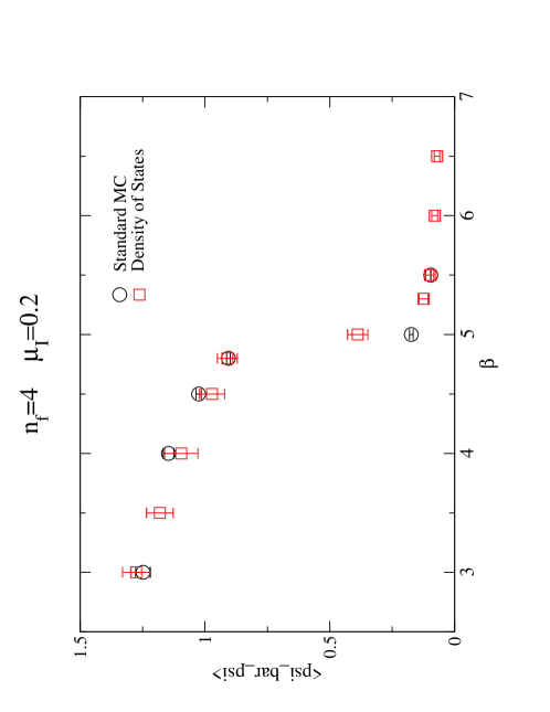
Figure 26: $<\bar{\psi}\psi>$ for $n_{f}=4$ on a $4^{4}$ lattice at $\mu_{I}=0.2$ and $m_{q}=0.025$. The standard Monte Carlo results were obtained by the R-algorithm[103]. Ref.TAKAISHI

5.5.2 Density of states of phase

Gocksch[99] used the complex phase of the determinant as the parameter for the density of states and studied the chiral condensate $\langle\bar{\Psi}\Psi\rangle$ and the phase diagram of QCD at infinite gauge coupling. In Ref. Gocksch he sets

$$x(U)=\theta(U),$$ (130)

$$g(U)=|\det\Delta(\mu)|e^{-\beta S_{g}}.$$ (131)

Then we obtain

$$\rho(E)=\int dU\delta(E-\theta(U))|\det\Delta(\mu)|e^{-\beta S_{g}},$$ (132)

$$\langle O\rangle=\frac{1}{Z_{\rho}}\int dE\rho(E)e^{iE}\langle O\rangle_{E},$$ (133)

$$Z_{\rho}=\int dE\rho(E)e^{iE}.$$ (134)

In order to obtain $\rho(E)$, simulations were carried out according to the probability $\displaystyle P(U)dU\sim|\det\Delta(\mu)|e^{-\beta S_{g}}dU$ and the histogram of $E$, which forms the density of state $\rho(E)$ in the end, was constructed. In the actual simulations, in order to speed up the process, the period of $E$ was divided into bins and the simulations were performed for each bin. Each bin has overlaps with the neighboring bins to match the adjacent density of states. The updating process is constrained in the range of each bin. Therefore the configuration leading out of the range is not accepted. Nevertheless the event has to be recorded in order to form the correct histogram[104].

5.5.3 Density of states of observable

One may use observables to form the density of states. In Refs. AmAnaNishiVer and [100] the random matrix theory for finite density QCD was studied by making use of the density of states for the quark number density. Originally they call the method ”factorization method” which is considered as a variety of the density of states method.

Setting

$$x(U)=O(U),$$ (135)

and

$$g(U)=|\det\Delta(\mu)|e^{-\beta S_{g}},$$ (136)

we obtain

$$\rho(E)=\int dU\delta(E-O(U))|\det\Delta(\mu)|e^{-\beta S_{g}},$$ (137)

$$\langle O\rangle=\frac{1}{Z_{\rho}}\int dE\rho(E)E\langle e^{i\theta}\rangle_{E},$$ (138)

$$Z_{\rho}=\int dE\rho(E)\langle e^{i\theta}\rangle_{E}.$$ (139)

If the operator $O$ takes a complex number, we may evaluate real and complex terms independently. First we rewrite $\langle O\rangle$ as

$$\langle O\rangle=\langle O_{R}\rangle+i\langle O_{I}\rangle$$ (140)

where $O_{R}$ and $O_{I}$ stand for ${\rm{Re}}(O)$ and ${\rm Im}(O)$ respectively. Then, defining the density of states $\rho_{R}(E)$ and $\rho_{I}(E)$ as

$$\rho_{R}(E)=\int dU\delta(E-O_{R})|\det\Delta(\mu)|e^{-\beta S_{g}},$$ (141)

$$\rho_{I}(E)=\int dU\delta(E-O_{I})|\det\Delta(\mu)|e^{-\beta S_{g}},$$ (142)

we obtain $\langle O_{R}\rangle$ and $\langle O_{I}\rangle$ as given bellow. For $i=R,I$,

$$\langle O_{i}\rangle=\frac{1}{Z_{i}}\int dE\rho_{i}(E)E\langle e^{i\theta}\rangle_{i,E}.$$ (143)

$$Z_{i}=\int dE\rho_{i}(E)\langle e^{i\theta}\rangle_{i,E},$$ (144)

where

$$\langle e^{i\theta}\rangle_{i,E}=\frac{1}{\rho_{i}(E)}\int dU\delta(E-O_{i})e^{i\theta}|\det\Delta(\mu)|e^{-\beta S_{g}}.$$ (145)

Finally the real part of $\langle O\rangle$ is given by

$${\rm{Re}}\langle O\rangle=\langle\tilde{O_{R}}\rangle-\langle\tilde{O_{I}}\rangle$$ (146)

where

$$\langle\tilde{O_{R}}\rangle=\frac{1}{C}\int dE\rho_{R}(E)E\langle\cos\theta\rangle_{R,E}$$ (147)

$$\langle\tilde{O_{I}}\rangle=\frac{1}{C}\int dE\rho_{I}(E)E\langle\sin\theta\rangle_{I,E}$$ (148)

and $C=Z_{R}=Z_{I}$. In Ref.[101], to obtain $\langle\cos\theta\rangle_{R,E}$ and $\langle\sin\theta\rangle_{I,E}$, they performed simulations with the constrained partition functions which are actually the density of states as given in Eq.(141) and (142). The density of states itself was also evaluated through those simulations. They argue that since the simulations are performed with the constrained partition function which forces the simulations to sample the important region, the results are obtained accurately.

5.6 Complex Langevin

Stochastic quantization by Parisi and Wu does not rely on the path integral, and its simulation is realized by the Langevin equation[106]. Parisi [107] and Klauder [108] proposed independently an extension of the Langevin algorithm to a system with a complex action.

For the dynamical variable $x$ which is subject to the (Euclidean) action $S(x)$, let us consider a stochastic process along the “fictitious” time $\tau$,

$$\frac{dx(\tau)}{d\tau}=-\frac{dS}{dx}+\eta(\tau),$$ (149)

where $\eta(\tau)$ is a Gaussian white noise characterized by $\langle\eta(\tau)\rangle=0$ and $\langle\eta(\tau)\eta(\tau^{\prime})\rangle=2\delta(\tau-\tau^{\prime})$. From the Langevin equation, we can derive an equivalent Fokker-Planck equation,

$$\frac{\partial}{\partial\tau}P(x;\tau)=\frac{\partial}{\partial x}\left(\frac{\partial}{\partial x}+\frac{dS}{dx}\right)P(x;\tau).$$ (150)

By virtue of the positive semi-definite property of the Fokker-Planck Hamiltonian, $H_{FP}=-\frac{\partial}{\partial x}(\frac{\partial}{\partial x}+\frac{dS}{dx})$, we can obtain a stationary solution as,

$$P(x,\tau)\smash{\mathop{\hbox to28.45274pt{\rightarrowfill}}\limits_{t\to\infty}}P_{eq}(x)\propto{\rm e}^{-S(x)}.$$ (151)

Therefore, putting the solution of the Langevin equation into the quantities $O(x)$ and taking the average over the ensemble of the random noise $\eta$, we can obtain the expectation value $\langle O(x)\rangle$ with probability measure $P_{eq}(x)\propto{\rm e}^{-S(x)}$. This is a rough sketch of the basic procedure of the stochastic quantization. In practical use, instead of an ensemble average, the long time average is taken over the simulation time $\tau$ after thermalization, where we assume ergodicity.

Once the action $S(x)$ becomes complex, the situation is not trivial. Putting a complex action into the above Langevin equation leads to the complex-valued extended version,

$$\frac{dz(\tau)}{d\tau}=-\frac{dS(z)}{dz}+\eta(\tau)$$ (152)

with a complex variable $z(\tau)=x(\tau)+iy(\tau)$ and real noise $\eta(\tau)$. The corresponding Fokker-Planck equation is defined for a complex distribution function $P_{\rm c}(x)$ of the real variable $x$ which satisfies,

$$\langle O(z(\tau))\rangle_{\eta}=\int dxP_{\rm c}(x)O(x).$$ (153)

In addition to the problem of the interpretation of the complex generalized distribution function $P_{\rm c}(x)$, in this case, Fokker-Planck Hamiltonian $H_{FP}$ loses the positive semi-definite property and there exists no general proof for the convergence.

However, if the spectrum of the Fokker-Planck Hamiltonian is composed of very small imaginary part and positive semi-definite real part, it is expected that a complete set ${z_{n}}$ with positive semi-definite eigenvalue ${E_{n}}$ and stationary solution ${\rm e}^{-S(z)}$ exist. For a simple case, this conjecture has been checked explicitly by Klauder and Petersen[109].

Karsch and Wyld applied the algorithm to a three dimensional SU(3) spin model with the chemical potential[110]. The Langevin simulations converge even for large values of the chemical potential, and are in agreement with exact solutions at the strong coupling limit.

Unfortunately the complex Langevin method sometimes gives incorrect results. For some simple noncompact variable case, the Parisi and Klauder algorithm can be proved to work well if the partition function satisfies certain conditions of the analytic behavior [111], but for the compact variable case, it is difficult to judge if the algorithm gives correct results or not.

Extensive use of the fictitious time as a redundant variable introducing a kernel in the Langevin equation has been discussed by the Waseda and Siegen group intensively[112]. A kernel $K(z)$ is introduced as,

$$\frac{dz(\tau)}{d\tau}=-K(z)\frac{dS}{dz}+\frac{dK}{dz}+\xi(\tau),$$ (154)

where $\xi(\tau)$ is a noise satisfying $\langle\xi(\tau)\rangle=0$ and $\langle\xi(\tau)\xi(\tau^{\prime})\rangle=2K(z)\delta(\tau-\tau^{\prime})$. The corresponding Fokker-Planck equation becomes,

$$\frac{\partial}{\partial\tau}P_{\rm c}(x;\tau)=-H_{FP}P_{\rm c}(x;\tau),$$ (155)

where

$$-H_{FP}=\frac{\partial}{\partial x}K(x)\left(\frac{\partial}{\partial x}+\frac{dS}{dx}\right).$$ (156)

Therefore, the role of the kernel is to change relaxation process only keeping the same asymptotic behavior,

$$P_{\rm c}(x,\tau)\smash{\mathop{\hbox to28.45274pt{\rightarrowfill}}\limits_{t\to\infty}}P_{eq}(x)\propto{\rm e}^{-S(x)}.$$ (157)

Thereby, a choice of the appropriate kernel may provide a better relaxation process without changing the physical result. Indeed in some cases, the use of a kernel improves the relaxation process and converges the random walk. For example, Okamoto et al. applied a constant kernel method to the polynomial model and succeeded in extending Klauder and Petersen’s convergent region in the complex eigenvalue space[114]. Though a pole in the second Rieman sheet sometimes leads the constant kernel method to an incorrect result, an appropriate choice of the field dependent kernel solves the problem in the case of the polynomial model[113]. For the simple models, the origin of the problems in the complex Langevin method is well analyzed and some answers with kerneled Langevin equation exist(see more details in Ref. Okano2). However, the general recipes for the complex system are still unclear and how to manage the finite density QCD is still open.

5.7 Finite isospin model

Imagine a system in which the chemical potentials of $u$ and $d$ quarks have the opposite signs to each other,

$$\mu_{u}=-\mu_{d}\equiv\mu$$ (158)

The system is called a finite isospin model [116] or the isovector model [39].

The fermion determinant of this system is

$$\det\Delta(\mu_{u})\det\Delta(\mu_{d})=\det\Delta(\mu)\det\Delta(-\mu)=|\det\Delta(\mu)|^{2}$$ (159)

where we use the relationship (14). Therefore the finite isospin model is considered as a two-flavor system where one drops the phase of the fermion determinant, and of course Monte Carlo calculation is possible.

Son and Stephanov have obtained the phase of the system shown in Fig.27[116], and the qualitative features of the diagram were confirmed by numerical simulation by Kogut and Sinclair [117]. See Figs. 28.

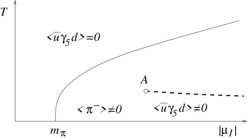
Figure 27: Finite Iso-spin phase diagram calculated by Son and Stephanov. (Ref. SONST).

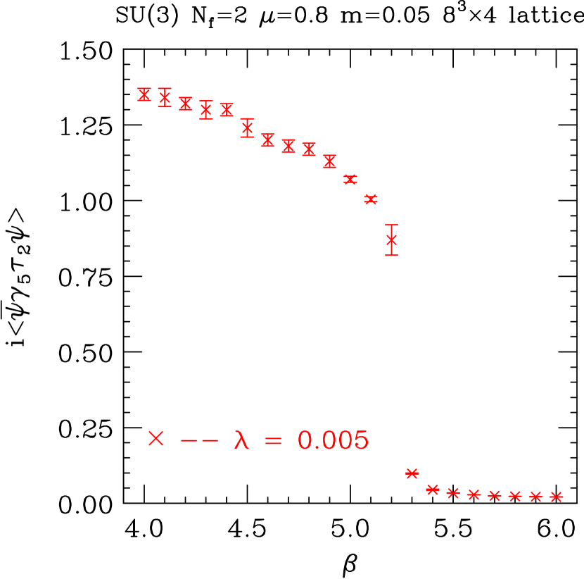
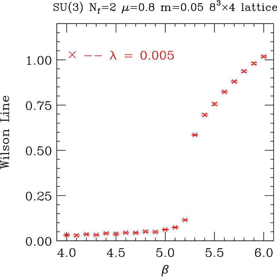
Figure 28: Numerical results of finite iso-spin model by Kogut and Sinclair. Left : $i\langle\bar{psi}\gamma_{5}\tau_{2}\psi\rangle$ at $\mu_{I}=0.8$ has finite value when the temperature is low, and decreases as $T$ increases. Right : Wilson line at $\mu_{I}=0.8$ at low $T$ is zero and increases when $T$ increases. (Ref. KoSi2002).

6 Summary

After the brief introduction of the lattice QCD actions with the chemical potential and their characters, we have seen many activities in the field. Recent progress in small $\mu$ and finite $T$ regions is very promising. Indeed until several years ago, we did not expect that any physically relevant data were provided by lattice QCD. This is the area which recent high energy heavy ion experiments are investigating. We anticipate now lattice data in the next several years which can be compared with experimental results. For that algorithm development is important.

Still it is difficult to study finite density QCD in large baryon density and low temperature regions, where many interesting phenomena such as color super condictivity and partial chiral restoration may occur. Two color QCD provides us hints on what may occur. Lattice simulations discussed in Sec.4 show us many interesting phenomena. Some of them are relevant for QCD and some not. In any case, they are interesting features in field theories and it is desirable to investigate their mechanisms.

We discussed many attempts in Sec.5 related with lattice field theory at finite density, i.e., 2-dimensional model, lattice NJL model, application of the strong coupling technique, density of state method, complex Langevin and finite isospin model. Surely there are more in the literature. We have made a survey of these works by hoping that a new idea appears from these studies, i.e., taking a lesson from the past.

Acknowledgement It is our pleasure to thank Prof. T. Kunihiro for providing us the chance to write this review and for continuous encouragement. We would like to thank Dr. S. Ejiri for many discussions, from which we have learned lots. We appreciate kind help by Prof. Y. Sasai for preparing the appendix. We are much indebted to Profs. T. Hatsuda, T. Inagaki, K. Okano and I. O. Stamatescu for many valuable discussions. We wish to thank Drs. K. Iida, S. Sasaki and M. Tachibana for providing us many facts and wisdoms on color super conductivity. This work is supported by DOE grants DE-FG02-96ER40495, Grant-in-Aide for Scientific Research by Monbu-Kagaku-sho (No.11440080, No. 12554008 and No. 13135216), and ERI, Tokuyama Univ.. Our simulations in this paper were performed on SR8000 at IMC, Hiroshima Univ., SX5 at RCNP, Osaka Univ., SR8000 at KEK..

Appendix A Gibbs formula to condense the fermion determinant

In lattice QCD simulations of finite baryon density system, we often need to calculate the fermion determinant. Gibbs has obtained a useful expression for this purpose. Here we describe a brief derivation of the formula following Gibbs,Hasen-To. Our proof given below is not very smart, but we hope that it helps the readers who need the formula.

We consider KS fermions,(19), and employ Eqs.(27),(28). The fermion matrix $\Delta$ is $(3\times N_{x}N_{y}N_{z}N_{t})^{2}$ complex matrix. We take the axial gauge as $U_{t}(x)=1$ except at $t=N_{t}-1$, the fermion matrix can be written in time slices as follows:

$$\Delta=\left(\begin{array}[]{c|c|ccc|c|c}B_{0}&{\bf 1}&0&\cdots&&0&U_{N_{t}-1}^{\dagger}{\rm e}^{-N_{t}\mu}\\ \hline\cr-{\bf 1}&B_{1}&{\bf 1}&\cdots&&0&0\\ \hline\cr 0&-{\bf 1}&B_{2}&\cdots&&&\\ \cdots&\cdots&\cdots&\cdots&\cdots&\cdots&\cdots\\ &&&\cdots&&{\bf 1}&0\\ \hline\cr 0&0&&\cdots&-{\bf 1}&B_{N_{t}-2}&{\bf 1}\\ \hline\cr-U_{N_{t}-1}{\rm e}^{N_{t}\mu}&0&&\cdots&0&-{\bf 1}&B_{N_{t}-1}\\ \end{array}\right)$$ (160)

where each column and row corresponds to the time slice $t=0,1,2,\cdots N_{t}-1$ and $U_{N_{t}-1}$ is the abbriviation of a $(N_{c}V_{s})\times(N_{c}V_{s})$ diagonal matrix whose elemets are $U_{t}(\vec{x},{N_{t}-1})\delta_{\vec{x},\vec{x}^{\prime}}$. Here we use the anti-periodic boundary condition along $t$ direction. The element of the above matrix is a $(N_{c}V_{s})\times(N_{c}V_{s})$ block matrix, where $V_{s}\equiv N_{x}N_{y}N_{z}$. $B_{i}$ stands for the spatial derivative and quark mass parts of the matrix at $i$-th time slice ($i=0,\cdots,N_{t}-1$). The chemical potential dependence has been summarized to the last time slice only. Let us denote $U_{N_{t}-1}{\rm e}^{N_{t}\mu}$ as $\Xi$ for the abbreviation.

Let us define $\tilde{\Delta}$ by multiplying $\Xi$ only to the last column of $\Delta$,

$$\tilde{\Delta}=\left(\begin{array}[]{ccccccc}B_{0}&{\bf 1}&&&&&{\bf 1}\\ -{\bf 1}&B_{1}&&&&&0\\ &-{\bf 1}&&&&&\\ &&\mbox{\quad}\ddots&&&&\\ &&&&&{\bf 1}&\\ &&&&&B_{N_{t}-2}&\Xi\\ -\Xi&0&&&&-1&B_{N_{t}-1}\Xi\\ \end{array}\right).$$ (161)

We assume that $N_{t}$ is even. Since

$$\det(\Xi)=\det(U_{N_{t}-1}{\rm e}^{N_{t}\mu})={\rm e}^{3V_{s}N_{t}\mu},$$ (162)

the determinant of $\tilde{\Delta}$ is related to $\det\Delta$ as $\det\tilde{\Delta}=\det\Delta{\rm e}^{3V_{s}N_{t}\mu}$. Multiplying the following matrix whose determinant is one,

$${\cal B}=\left(\begin{array}[]{cccccccc}{\bf 1}&B_{0}&0&&&&&\\ 0&{\bf 1}&0&&&&&\\ &&{\bf 1}&B_{2}&&&&\\ &&&{\bf 1}&&&&\\ &&&&\ddots&&&\\ &&&&&&0&0\\ &&&&&&{\bf 1}&B_{N_{t}-2}\\ &&&&&&&{\bf 1}\\ \end{array}\right),$$

to the fermion matrix $\tilde{\Delta}$ from the left, we obtain,

$${\cal B}\times\tilde{\Delta}$$ (170)

$$= \left(\begin{array}[]{ccccccccc}0&1+B_{0}B_{1}&B_{0}&0&&&1\\ -1&B_{1}&1&0&&&0\\ 0&-1&0&1+B_{2}B_{3}&B_{2}&&\\ &0&-1&B_{3}&1&&\\ &&&&\ddots&&\\ -B_{N_{t}-2}\Xi&&&&&0&(1+B_{N_{t}-2}B_{N_{t}-1})\Xi\\ -\Xi&&&&&-1&B_{N_{t}-1}\Xi\\ \end{array}\right).$$

Permuting the first column to the last and multiplying -1 to the last column, $\det{\tilde{\Delta}}$ is rewritten as,

$$\det\left(\begin{array}[]{ccccccccc}1+B_{0}B_{1}&B_{0}&0&&&1&0\\ B_{1}&1&0&&&0&1\\ -1&0&1+B_{2}B_{3}&B_{2}&&&0\\ 0&-1&B_{3}&1&&&\\ &&&\ddots&&&\\ &&&&0&(1+B_{N_{t}-2}B_{N_{t}-1})\Xi&B_{N_{t}-2}\Xi\\ &&&&-1&B_{N_{t}-1}\Xi&\Xi\\ \end{array}\right).$$

Denoting as,

$$\Omega_{j,j+1}=\left(\begin{array}[]{cc}B_{j}B_{j+1}+1&B_{j}\\ B_{j+1}&1\end{array}\right)=\left(\begin{array}[]{cc}B_{j}&1\\ 1&0\end{array}\right)\left(\begin{array}[]{cc}B_{j+1}&1\\ 1&0\end{array}\right),$$ (171)

and

$$1_{2}=\left(\begin{array}[]{cc}1&0\\ 0&1\end{array}\right)$$ (172)

the determinant of the fermion matrix can be written as,

$$\det(\tilde{\Delta})=\det\left(\begin{array}[]{ccccccc}\Omega_{01}&&&&1_{2}\\ -1_{2}&\Omega_{23}&&&\\ &-1_{2}&\Omega_{45}&&\\ &&\ldots&&\\ &&&-1_{2}&\Omega_{N_{t}-2,N_{t}-1}\Xi\\ \end{array}\right).$$ (173)

Note that $\Omega_{N_{t}-2,N_{t}-1}\Xi$ is $(3V_{s}\times 2)$ times $(3V_{s}\times 2)$ matrix.

We multiply a matrix of which determinant is 1 from the right.

$$\det(\tilde{\Delta}) = \det\left(\begin{array}[]{ccccccc}\Omega_{01}&&&&1_{2}\\ -1_{2}&\Omega_{23}&&&\\ &-1_{2}&\Omega_{45}&&\\ &&\ldots&&\\ &&&-1_{2}&\Omega_{N_{t}-2,N_{t}-1}\Xi\\ \end{array}\right)\left(\begin{array}[]{ccccccc}1_{2}&&&&-\Omega_{01}^{-1}\\ &1_{2}&&&\\ &&1_{2}&&\\ &&&\ldots&\\ &&&&1_{2}\\ \end{array}\right)$$ (184)

$$= \det\left(\begin{array}[]{ccccccc}\Omega_{01}&0&\ldots&0&0\\ -1_{2}&\Omega_{23}&&&\Omega_{01}^{-1}\\ &-1_{2}&\Omega_{45}&&\\ &&\ldots&&\\ &&&-1_{2}&\Omega_{N_{t}-2,N_{t}-1}\Xi\\ \end{array}\right)$$ (190)

$$= \det(\Omega_{01})\det\left(\begin{array}[]{ccccccc}\Omega_{23}&&&\Omega_{01}^{-1}\\ -1_{2}&\Omega_{45}&&\\ &\ldots&&\\ &&-1_{2}&\Omega_{N_{t}-2,N_{t}-1}\Xi\\ \end{array}\right)$$

$$= \cdots$$

$$= \det\left(\Omega_{01}\Omega_{23}\cdots\Omega_{{N_{t}-6},{N_{t}-5}}\right)$$

$$\times \begin{array}[]{|cc|}\Omega_{N_{t}-4,N_{t}-3}&0\\ -1&\Omega_{N_{t}-2,N_{t}-1}\Xi+(\Omega_{01}\cdots\Omega_{Nt-3,N_{t}-2})^{-1}\\ \end{array}$$ (198)

where we used a formula for blocked matrixes $A_{ij}$:

$$\begin{array}[]{|cccc|}A_{11}&0&\ldots&0\\ A_{21}&A_{22}&\ldots&A_{2n}\\ \vdots&\vdots&&\vdots\\ A_{n1}&A_{n2}&\ldots&A_{nn}\\ \end{array}=\left|A_{11}\right|\begin{array}[]{|ccc|}A_{22}&\ldots&A_{2n}\\ \vdots&&\vdots\\ A_{n2}&\ldots&A_{nn}\\ \end{array}.$$ (199)

Taking the similar step recursively, we can reduced the matrix up to two-time slices. We obtain finally,

$$\begin{array}[]{cll}\det(\Delta)&=&\det\tilde{\Delta}\times e^{-3V_{s}N_{t}\mu}\\ &=&\det(1+e^{N_{t}\mu}P)\times e^{-3V_{s}N_{t}\mu}\\ \\ &=&\det\left\{e^{N_{t}\mu}(e^{-N_{t}\mu}+P)\right\}\times e^{-3V_{s}N_{t}\mu}\\ \\ &=&\det\left(P+e^{-N_{t}\mu}\right)\times(e^{3V_{s}N_{t}\mu})^{2}\times e^{-3V_{s}N_{t}\mu}\\ \\ &=&\det\left(P+e^{-N_{t}\mu}\right)\times e^{3V_{s}N_{t}\mu},\end{array}$$ (200)

where

$$P=\displaystyle\left(\Pi_{j=0,2,4}^{N_{t}-2}\Omega_{j,j+1}\right)U_{N_{t}-1}\\ =\displaystyle\left(\Pi_{j=0}^{N_{t}-1}\left(\begin{array}[]{cc}B_{j}&1\\ 1&0\\ \end{array}\right)\right)U_{N_{t}-1}.$$ (201)

The rank of the matrix $P+e^{-N_{t}\mu}$ is $3\times(2V_{s})$. Therefore if $N_{t}>2$, we obtain a condensed smaller matrix. To estimate the determinant, $LU$ decomposition is fastest for small size lattices on many computers if there is enough memory. If we have eigenvalues of the matrix $P$, $\{\lambda_{i}\}$, which do not depend on the chemical potential $\mu$, we obtain Eq.(49), which gives us values of the fermion determinant at any $\mu$.

Appendix B Meson and baryon propagators in color SU(2) space

A $\bar{q}-{q}$ bound state belonging to 1 representation in $\bar{\bf 2}\otimes{\bf 2}$ is called a meson. With a quark field $\psi(x)$, the meson operators are constructed as

$$\bar{\psi}\Gamma\psi,$$

with $\Gamma$ being Dirac’s $\gamma$ matrices. $\Gamma=1$ corresponds to a scalar meson, $\Gamma=\gamma_{5}$ corresponds to a pseudoscalar meson, $\Gamma=\gamma_{\mu}$ corresponds to a vector meson, and $\Gamma=\gamma_{5}\gamma_{\mu}$ to an axial vector meson.

In SU(2), 1 representation also exists in ${\bf 2}\otimes{\bf 2}$ and $q-q$ bound state can be realized as a color singlet state. It means that a baryon in SU(2) theory is a color singlet di-quark state. On this point, color-SU(2) and color-SU(3) are essentially different. The di-quark operator is given as,

$$\varepsilon^{ab}{\psi_{a}}^{T}C\Gamma\hat{\tau}\psi_{b},$$

with $a$ and $b$ being color indices. $\hat{\tau}$ stands for Pauli matrix $\tau_{2}$ or $\vec{\tau}\tau_{2}$ in the flavor SU(2) space. In order to satisfy the fermionic property of the quark, the di-quark state must be totally antisymmetric utilizing flavor degrees of freedom. We must take iso-singlet channel, $\hat{\tau}=\tau_{2}$, for $\Gamma=1$, $\gamma_{5}$ and $\gamma_{\mu}\gamma_{5}$. Iso-vector di-quarks are realized for the vector channel, $\Gamma=\gamma_{\mu}$. Because of the charge conjugation $C$, we must turn our attention to the parity of the di-quark states; $\Gamma=1$ corresponds to a pseudoscalar di-quark, $\Gamma=\gamma_{5}$ corresponds to a scalar di-quark, $\Gamma=\gamma_{\mu}$ corresponds to an axial vector di-quark, and $\Gamma=\gamma_{5}\gamma_{\mu}$ to a vector di-quark.

By virtue of the simple structure of SU(2), propagators of meson and di-quark are degenerate in a vacuum state, i.e. , propagators of pseudoscalar meson and scalar di-quark, and vector meson and axial vector di-quark are degenerate.

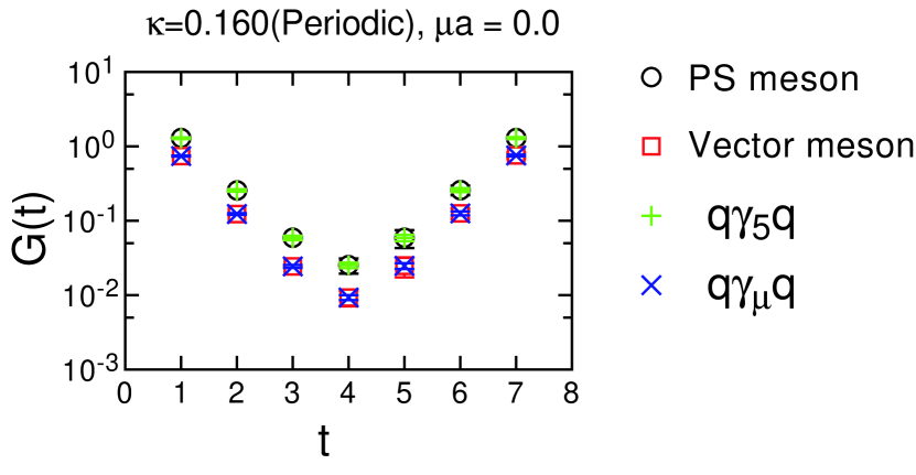
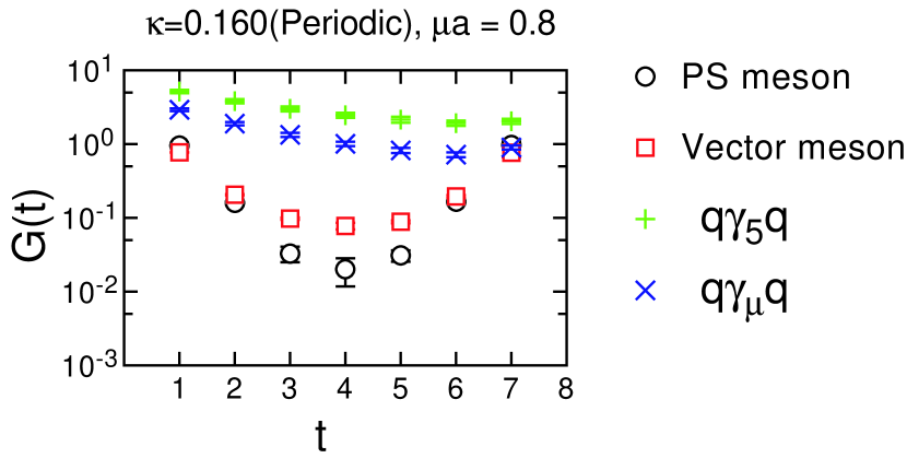
Figure 29: Hadron propagators at $\mu a=0$ (left) and $\mu a=0.8$ (right). Pseudoscalar and vector mesons and scalar and axial vector baryons are shown.

Figure (29) shows the propagators on a $4^{3}\times 8$ lattice with spatially periodic boundary condition at $\beta=0.7$ and $\kappa=0.150$. At $\mu=0$ (29a), pseudoscalar meson and scalar di-quark, and vector boson and axial vector di-quark are degenerate. With the finite $\mu$, the $\mu B$ term in the $W$ makes the di-quark propagators asymmetric in the time-direction. On the other hand, the meson propagators keep the symmetric shape. Therefore, degeneracy between the meson propagator and di-quark propagators is solved with finite $\mu$.

The asymmetry of the di-quark propagator is caused by the difference of the charge of ”di-quark” and ”anti-di-quark”. The chronological propagation is provided by a particle with charge $Q$ and of which the chemical potential is $\mu Q$. On the other hand, the anti-chronological propagation is governed by an anti-particle with charge $-Q$ and which is affected by the chemical potential as $-\mu Q$. Taking this asymmetry into account, we adopt

$$G_{d}(t)=C_{1}{\rm e}^{-(m-2\mu)t}+C_{2}{\rm e}^{-(m+2\mu)(N_{t}-t)}$$

as a fitting function to the di-quark propagator, where $C_{1}$ and $C_{2}$ must keep the constraint on the bosonic boundary condition of di-quark. For the mesons, even in finite density we can use a usual form as,

$$G_{m}{t}=C_{1}{\rm e}^{-mt}+C_{2}{\rm e}^{-m(N_{t}-t)}.$$

Appendix C Thermodynamical variables on the lattice

The path integral form of the partition function is given as [31] ,

$$Z = {\rm{Tr}}({\rm e}^{-\beta(H-\mu N)})$$

$$= \int\mathcal{D}U\mathcal{D}\bar{\psi}\mathcal{D}\psi{\rm e}^{-\int_{0}^{\beta}d\tau\int d^{3}x(L+\mu n)}$$

$$= {\rm e}^{-\beta(\epsilon-\mu n)V},$$

The energy density $\epsilon$, and the number density $n$ are given by

$$\epsilon = \frac{1}{V}\left(-\frac{\partial}{\partial\beta}+\frac{\mu}{\beta}\frac{\partial}{\partial\mu}\right)\log Z|_{V},$$

$$n = \frac{1}{\beta V}\frac{\partial}{\partial\mu}\log Z|_{V},$$ (203)

On the lattice, $\beta=N_{t}a_{t}$, and

$$\frac{\partial}{\partial\beta}=\frac{1}{N_{t}}\frac{\partial}{\partial a_{t}}$$ (204)

We must be careful that the temperature, $T$, changes when we vary the lattice spacing $a_{t}$ which is a function of the coupling constant.

A simple and safe way is to write down a formula in terms of non-dimensional quantities and to start to calculate. For example, the number density is given in the continuum world as

$$n=\frac{\partial p}{\partial\mu}=\frac{\partial}{\partial\mu}\left(\frac{T}{V}\log Z\right)$$ (205)

We may write a formula

$$\frac{n}{T^{3}}=\frac{N_{t}^{3}}{N_{s}^{3}}\frac{\partial}{\partial\hat{\mu}}\log Z,$$ (206)

where

$$\hat{\mu}\equiv\frac{\mu}{T}.$$ (207)

References

- [1] I. M. Barbour, S. E. Morrison, E. G. Klepfish, J. B. Kogut and M-P. Lombardo, Nucl. Phys. Proc. Suppl. 60A, 220-234, 1998, hep-lat/9705042.
- [2] S. Hands, Nucl.Phys.Proc.Suppl. 106 (2002) 142, hep-lat/0109034
- [3] J. B. Kogut, hep-lat/0208077, to appear in Nucl. Phys. Proc. Suppl.
- [4] M-P. Lombardo, hep-lat/0210040.
- [5] F.Karsch and E.Laermann, hep-lat/0305025, to appear in ”Quark-Gluon Plasma III”, R.Hwa (ed.).
- [6] B.C. Barrois Nucl.Phys.B129 (1977) 390, D. Bailin and A. Love, Phys.Rep. 107 (1984) 325. M. Iwasaki and T. Iwado, Phys.Lett. B350 (1995) 163,
- [7] M. Alford, K. Rajagopal and F. Wilczek, Phys. Lett. B422(1998) 247.
- [8] R. Rapp, T. Schaefer, E. V. Shuryak and M. Velkovsky, Phys. Lett. 81 (1998) 53.
- [9] M.Kitazawa, T.Koide, T.Kunihiro, Y.Nemoto, Phys.Rev. D65 (2002) 091504, (nucl-th/0111022)
- [10] M. Alford, K. Rajagopal and F. Wilczek, Nucl.Phys. B537 (1999) 443.
- [11] M. Alford, J. Bowers and K. Rajagopal, hep-ph/0008208, Phys.Rev. D63 (2001) 074016
- [12] D. T. Son, Phys. Rev. D59 (1999), 094019
- [13] K. Rajagopal and F. Wilczek, “At the frontier of Particle Physics - Handbook of QCD”, ed. by M. Shifman, Vol. 4, Chap.35, World Scientific, 2002. hep-ph/0011333.
- [14] R.D. Pisarski and D.H. Rischke, Phys.Rev. D60 (1999) 094013, nucl-th/9903023
- [15] CERES/NA44 Collaboration, G. Agakichiev et al., Phys.Lett. B422 (1998) 405-412; (nucl-ex/9712008). H. Appelshaeuser, talk at “Compressed Baryonic Matter Workshop, 2002”, J. P. Wessels, talk at Quark Matter 2002, nucl-ex/0212015. See also R. Rapp and J. Wambach, Adv. Nucl. Phys. 25 (2000). hep-ph/9909229
- [16] K. Ozawa et al., Phys. Rev. Lett. 86 (2001) 5019, nucl-ex/0011013.
- [17] P. Fachini, (STAR Collaboration) nucl-ex/0211001.
- [18] Suzuki et al., nucl-ex/0211023
- [19] T. Kunihiro, hep-ph/0111121, “The Sigma Meson and Chiral Transition in Hot and Dense Matter” Invited talk given at the IXth International Conference on Hadron Spectroscopy- HADRON 2001. P. 315 in “Hadron Spectroscopy – Ninth International Conference on Hadron Spectroscopy, Protovino Russia, 25 August – 1 September 2001”, ed. by D. Amelin and A. M. Zaitsev, (AIP conference proceedings vol. 619, Melville, New York, 2002)
- [20] M. Lutz, S. Klimt and W. Weise, Nucl. Phys. A542 (1992) 521.
- [21] R. Hagedorn, Suppl. Nuovo Ciment 3, 147-186, (1956); R. Hagedron and J. Rafelski Phys. Lett., 97B, 136 (1980).
- [22] N. Cabbibo and G. Parisi, Phys. Lett. 59B, 67 (1975).
- [23] L. D. McLerran and B. Svetitsky, Phys. Lett. 98B, 195 (1981); Phys. Rev. D24, 450 (1981).
- [24] J. Kuti, J. Polonyi and K. Szlachanyi, Phys. Lett, 98B 199 (1981).
- [25] K. Kanaya, hep-ph/0209116, to appear in Proceed. QM02.
- [26] A. Nakamura, Phys. Lett. 149B (1984) 391.
- [27] S. Morrison and S. Hands, hep-lat/9902012
- [28] S. Hands, J. B. Kogut, M.-P. Lombardo and S. E. Morrison, Nucl. Phys. B558 (1999) 327, hep-lat/9902034.
- [29] I. Barbour, N. E., Behilil, E. Dagotto, F. Karsch, A. Moreo, A. Stone and H. W. Wyld, Nucl. Phys. B275[FS17] (1986) 296.
- [30] M. A. Stephanov, Phys. Rev. Lett. 76, 4472 (1996).
- [31] D. J. Gross, R. D. Pisarski, L. G. Yaffe, Rev. Mod. Phys. 53, 43 (1981).
- [32] P. Hasenfratz and F. Karsch, Phys. Lett. 125B (1983) 308.
- [33] R. V. Gavai, Phys. Rev. D32, (1985), 519.
- [34] M. Creutz, hep-lat/9905024.
- [35] A. Nakamura, Nucl. Phys. B (Proc. Suppl. )17 (1990) 395.
- [36] D. Toussaint, Nucl. Phys. B (Proc. Suppl. ) 17 (1990) 539.
- [37] A. Hasenfratz and D. Toussaint, Nucl. Phys B371 (1992) 539.
- [38] S. Gottlieb et al., Phys. Rev. D 55, 6852 (1997), hep-lat/9612020
- [39] QCD-TARO Collaboration: S. Choe, Ph. de Forcrand, M. Garcia Perez, S. Hioki, Y. Liu, H. Matsufuru, O. Miyamura, A. Nakamura, I. -O. Stamatescu, T. Takaishi, T. Umeda, Phys. Rev. D65, 054501 (2002).
- [40] Z. Fodor, S. D. Katz, JHEP 0203 (2002) 014, (hep-lat/0106002).
- [41] C. R. Allton, S. Ejiri, S. J. Hands, O. Kaczmarek, F. Karsch, E. Laermann, Ch. Schmidt, L. Scorzato (Bielefeld-Swansea), Phys. Rev. D66 074507 (2002), (hep-lat/0204010).
- [42] C. R. Allton, S. Ejiri, S. J. Hands, O. Kaczmarek, F. Karsch, E. Laermann and Ch. Schmidt (Bielefeld-Swansea), hep-lat/0305007.
- [43] Z. Fodor, S.D. Katz and K.K. Szabo, hep-lat/0208078
- [44] M. D’Elia, M. P. Lombardo, Proceedings of the GISELDA Meeting held in Frascati, Italy, 14-18 January 2002, hep-lat/0205022.
- [45] Ph. de Forcrand, O. Philipsen, Nucl. Phys. B642 290 (2002), hep-lat/0205016.
- [46] F. Csikor, G. I. Egri, Z. Fodor, S. D. Katz, K. K. Szabo, A. I. Toth, (hep-lat/0301027, hep-lat/0209114).
- [47] B.Müller, Nucl. Phys. A 702 (2002) 281; V.Koch, M.Bleicher and S.Jeon, Nucl. Phys. A 702 (2002) 291; R.V.Gavai, Nucl. Phys. A 702 (2002) 299; N. Sasaki, O. Miyamura, S. Muroya and C. Nnonaka, Europhys. Lett. 54, (2001) 38.
- [48] S.Gottlieb et.al., Phys. Rev. D 55 (1997) 6852
- [49] R.V.Gavai, J.Potvin and S.Sanielevici,Phys. Rev. D 40 (1989) 2743
- [50] R.V.Gavai and S.Gupta, Phys. Rev. D 64 (2001) 074506;Phys. Rev. D 65 (2002) 094515
- [51] R.V.Gavai, S.Gupta and P.Majumdar, Phys. Rev. D 65 (2992) 054506
- [52] C.Bernard et. al., hep-lat/0209079
- [53] R.V. Gavai and S. Gupta, hep-lat/0303013
- [54] I.M.Barbour, Nucl. Phys. (PS) 60A (1998) 229.
- [55] P.E. Gibbs Phys. Lett., B172 (1986) 53.
- [56] S. Ejiri, hep-lat/0212022.
- [57] Ph. de Forcrand, S. Kim and T. Takaishi hep-lat/0209126
- [58] A. Roberge and N. Weiss, Nucl. Phys. B275[FS17] (1986) 734-745.
- [59] M. -P. Lombardo, hep-lat/9907025.
- [60] R. Aloisio, V. Azcoiti, G. Di Carlo, A. Galante and A. F. Grillo, Phys. Lett. B493 189 (2000), (hep-lat/0009034).
- [61] J. B. Kogut, D. Toublan, D. K. Sinclair, Phys. Lett. B514 (2001) 77, (hep-lat/0104010).
- [62] J. B. Kogut, D. K. Sinclair, S. J. Hands, S. E. Morrison, Phys. Rev. D64 (2001) 094505, (hep-lat/0105026).
- [63] J. B. Kogut, D. Toublan, D. K. Sinclair, Nucl. Phys. B642 (2002) 181, (hep-lat/0205019).
- [64] S. Muroya, A. Nakamura, C. Nonaka, Nucl. Phys. Proc. Suppl. 94 (2001) 469, (hep-lat/001007).
- [65] S. Muroya, A. Nakamura, C. Nonaka, Phys. Lett. B551 (2003) 305 (hep-lat/0211010), Nucl. Phys. Proc. Suppl. 106 (2002) 453, (hep-lat/0111032), hep-lat/0208006.
- [66] Y.Liu, O.Miyamura, A.Nakamura and T.Takaishi, Proceedings of the International Workshop on Nonperturbative Methods and Lattice QCD, Guangzhou, China (hep-lat/0009009)
- [67] J.B.Kogut, M.A.Stephanov and D.Toublan, Phys. Lett. B464 (1999) 183-191.
- [68] J.B. Kogut, M.A. Stephanov, D. Toublan, J.J.M. Verbaarschot and A. Zhitnitsky Nucl. Phys. B582 (2000) 477 (hep-ph/0001171)
- [69] S. Hands, I. Montvay, S. Morrison, M. Oevers, L. Scorzato and J. Skullerud, Eur.Phys.J. C17 (2000) 285-302, hep-lat/0006018
- [70] G. E. Brown and M. Rho, Phys. Rev. Lett. (1991) 2720.
- [71] T. Hatsuda and S. H. Lee, Phys. Rev. C46 (1992) R34.
- [72] M. Harada et al., hep-ph/0111120.
- [73] K. Yokokawa et al., hep-ph/0204163.
- [74] S. Muroya, A. Nakamura, C. Nonaka, Phys. Lett. B551 (2003) 305-310, hep-lat/0211010.
- [75] S. Hands, J. B. Kogut, C. G. Strouthos and T. N. Tran, hep-lat/0302021
- [76] D. J. Gross and A. Neveu, Phys. Rev. D10, 3235,(1974)
- [77] S. Coleman, “Aspects of Symmetry”, Cambridge Univ. Press, 1985.
- [78] A. B. Zamolodchikov and A. B. Zamolodchikov, Annals of Phys. 120 (1979), 253.
- [79] A. Chodos, H. Minakata, F. Cooper, A. Singh and W. Mao, hep-ph/0009019.
- [80] U. Wolff, Phys. Lett. 157B (1985) 303.
- [81] T. Inagaki, K. Kouno and T. Muta, Int. J. Mod. Phys. A10, 2241, (1995).
- [82] F. Karsch, J. Kogut and H. W. Wyld, Nucl. Phys. B280[FS18] 1987, 289.
- [83] T. Izubuchi, J. Noaki and A. Ukawa, Phys.Rev. D58 (1998) 114507, hep-lat/9805019.
- [84] S. Hands and D. H. Walters, Phys. Lett. B 548(2002)196.
- [85] S. J. Hands, B. Lucini and S. E. Morrison, Phys. Rev. Lett. 86 (2001) 753; S. J. Hands, B.Lucini and S. E. Morrison, Phys. Rev. D65(2002)036004.
- [86] E. -M. Ilgenfritz and J. Kripfganz, Z. Phys. C29 (1985), 79.
- [87] P. H. Damgaard, D. Hocheberg and N. Kawamoto Phys.Lett. B158 (1985) 239
- [88] N. Bilić, K. Demeterfi and B. Petersson, Nucl.Phys. B377, (1992) 615
- [89] Y. Nishida, K. Fukushima and T. Hatsuda, hep-ph/0306066, to appear in the Hidenaga Yamagishi Commemorative volume of Physics Reports, ed. E. Witten and I. Zahed
- [90] P. Rossi and U. Wolff, Nucl. Phys. B248 (1984) 105.
- [91] F. Karsch and K.H.Mütter, Nucl. Phys. B313 (1989) 541.
- [92] I. Barbour, N.-E. Behilil, E. Dagotto, F. Karsch, A. Moreo, M. Stone and H.W. Wyld, Nucl. Phys. B275 (1986) 296.
- [93] R. Aloisi, V. Azcoiti, G. Di Carlo, A. Galante, A.F. Grillo. Nucl. Phys. B564, 489, 2000, hep-lat/9910015
- [94] I. M. Barbour, S. E. Morrison, E. G. Klepfish, J. B. Kogut, M-P. Lombardo, Phys. Rev. D56, 7063, 1997, hep-lat/9705038.
- [95] S. Chandrasekharan, Phys.Lett.B536:72-78,2002 hep-lat/0203020
- [96] D. E. Miller and K. Redlich, Phys. Rev. D35, (1987) 2524-2530.
- [97] J. Engels, O. Kaczmarek, F. Karsch and E. Laermann, Nucl.Phys. B558 (1999) 307-326, hep-lat/9903030; O. Kaczmarek, hep-lat/9905022, “Understanding Deconfinement in QCD”, ECT* Trento, March 1999.
- [98] X.Q. Luo, Mod.Phys.Lett. A16 (2001) 1615
- [99] A. Gocksch, Phys. Rev. Lett. 61 (1988) 2054.
- [100] K.N.Anagnostopoulos and J.Nishimura, hep-th/0108041
- [101] J.Ambjorn, K.N.Anagnostopoulos, J.Nishimura and J.J.M.Verbaarschot, hep-lat/0208025
- [102] V.Azcoite, G.Di Carlo and A.F.Grillo, Phys. Rev. Lett. 65 (1990) 2239
- [103] S.Gottlieb et.al., Phys. Rev. D35 (1987) 2531
- [104] G.Bhanot, K.Bitar and R.Salvador, Phys. Lett. B 187(1987) 381; Phys. Lett. B188 (1987) 246 M.Karliner, S.R.Sharpe and Y.F.Chang, Nucl. Phys. B302 (1988) 204
- [105] T.Takaishi, in preparation
- [106] M. Namiki,“Stochastic Quantization”, Spriger Verlag Berlin Heidelberg 1992.
- [107] G. Parisi, Phys. Lett. 131B (1983),393.
- [108] J. R. Klauder, Phys. Rev. A29 (1984),2036.
- [109] L. R. Klauder and W. P. Petersen, J. Stat. Phys., 39(1985),53
- [110] F. Karsch and H. Wyld, Phys. Rev. Lett.21(1985),2242.
- [111] T. Matsui and A. Nakamura, Phys. Lett. B194(1987),262
- [112] N. Namiki and K. Okano, Prog. Theor. Phys. Suppl. 111(1993),1.
- [113] K. Okano, L. Schülke and B. Zheng, Prog. Theor. Phys. Suppl. 111(1993),313.
- [114] H. Okamoto, K. Okano, Lothar Schülke and S. Tanaka, Nucl. Phys. B324(1989),684.
- [115] K. Okano, L. Schülke and B. Zheng, Phys. Lett. B258(1991),42; K. Fujimura, K. Okano, L. Schülke, K. Yamagishi and B. Zheng, Nucl. Phys. B424[FS](1994),675.
- [116] D.T. Son and M.A. Stephanov, Phys. Rev. Lett. 86 (2001) 592
- [117] J.B. Kogut and D.K. Sinclair Phys. Rev. D 66 (2002) 034505; hep-lat/0209054