Chiral perturbation theory with Wilson-type fermions including $a^{2}$ effects: $N_{f}=2$ degenerate case

Abstract

We have derived the quark mass dependence of $m_{\pi}^{2}$, $m_{\rm AWI}$ and $f_{\pi}$, using the chiral perturbation theory which includes the $a^{2}$ effect associated with the explicit chiral symmetry breaking of the Wilson-type fermions, in the case of the $N_{f}=2$ degenerate quarks. Distinct features of the results are (1) the additive renormalization for the mass parameter $m_{q}$ in the Lagrangian, (2) $O(a)$ corrections to the chiral log ($m_{q}\log m_{q}$) term, (3) the existence of more singular term, $\log m_{q}$, generated by $a^{2}$ contributions, and (4) the existence of both $m_{q}\log m_{q}$ and $\log m_{q}$ terms in the quark mass from the axial Ward-Takahashi identity, $m_{\rm AWI}$. By fitting the mass dependence of $m_{\pi}^{2}$ and $m_{\rm AWI}$, obtained by the CP-PACS collaboration for $N_{f}=2$ full QCD simulations, we have found that the data are consistently described by the derived formulae. Resumming the most singular terms $\log m_{q}$, we have also derived the modified formulae, which show a better control over the next-to-leading order correction.

I Introduction

One of the most serious systematic uncertainties in the current lattice QCD simulations is caused by the chiral extrapolation. Due to the limitation of the current computational power, one can not perform simulations directly at the physical light quark(up and down) mass. Instead, one has performed simulations at several heavier quark masses and has extrapolated results to the physical quark mass point, using the polynomial(linear, quadratic, etc.) or the formula derived from the chiral perturbation theory (ChPT)ChPT . These extrapolations cause large systematic uncertainties, in particular in the case of full QCD simulations, where the lightest quark mass employed in the current QCD simulations is roughly half of the physical strange quark mass ($m_{\pi}/m_{\rho}\simeq 0.6$).

Recently more serious problem has been pointed out, in particular for full QCD simulations with Wilson-type quarks: the expected chiral behaviour predicted by the ChPT has not been observed. For example, the behaviour of the pion mass $m_{\pi}^{2}$ as a function of quark mass $m_{q}$ is given by

$$m_{\pi}^{2} = Am_{q}[1+\frac{Am_{q}}{16\pi^{2}N_{f}f_{\pi}^{2}}\log(Am_{q}/\Lambda^{2})],$$ (1)

where $\Lambda$ is some scale parameter. Since the pion decay constant is experimentally known as $f_{\pi}=93$ MeV, only $A$ and $\Lambda$ are unknown parameters. Unfortunately, such a two parameter fit can not explain lattice data well, which looks almost linear in the simulated range of quark masses. If one includes $f_{\pi}$ as a free parameter, the best fit typically gives $f_{\pi}^{2}\geq 5\times$ (93 MeV)²panel .

The most widely accepted interpretation for this discrepancy is that the simulated range of quark masses in the current simulations is still too heavy to apply the ChPT. If this interpretation is true, the current lattice simulations with the (Wilson-type) dynamical quarks lose a large part of their powers to predict properties of hadrons at the physical light quark masses.

In this paper, we investigate a theoretically more natural alternative that the explicit breaking of the chiral symmetry by the Wilson-type quark action modifies the formulae of the ChPT at the finite lattice spacing. We first derive formulae in the modified chiral perturbation theory for the Wilson-type quark action, denoted by WChPT in this paper. Such attempts have been made before at the leading orderSS and the next-to-leading orderRS . At the leading orderSS , the WChPT predicts the existence of the parity-flavor breaking phase transitionaoki1 ; aoki2 ; aoki3 for the 2 flavor QCD as long as massless pions appear at the critical quark mass. This analysis has also shown that the $O(a^{2})$ chiral breaking term play an essential role to generate the parity-flavor breaking phase transition, which is necessary to explain the existence of the massless pions for the Wilson-type quark actionaoki1 ; aoki2 ; aoki3 . In the next-to-leading order analysisRS , however, only the $O(a)$ breaking effects are included, and it is concluded that the effect of the chiral symmetry breaking can always be absorbed in the redefinition of the quark mass, so that all formulae in the ChPT remain the same if one replaces the quark mass $m_{q}$ with $m_{q}-m_{c}$, where $m_{c}$ is the additive $O(a)$ counter-term for the quark mass. In the section II, we perform the next-to-leading order calculation in the WChPT including $O(a^{2})$ chiral symmetry breaking effects. To make the difference between WChPT and ChPT clear, we consider only the case of the $N_{f}=2$ QCD with degenerate quark masses, and derive the formulae for mass and decay constant of the pion as well as the axial Ward-Takahashi identity quark mass, as a function of the “quark mass” in the effective theory. In section III, the derived formulae are applied to data of pion mass and the axial Ward-Takahashi identity quark mass calculated by the CP-PACS collaborationcppacs . We show that data are consistent with the formulae. We have attempted the resummation of the most singular term, and have derived the modified formulae in section IV. Our conclusions and discussions are given in section V.

II Wilson Chiral Perturbation Theory

II.1 Derivation of effective Lagrangian

It is difficult to derive the effective chiral Lagrangian for mesons directly from lattice QCD with the Wilson-type quarks using the symmetry, since the quark mass requires a counter term $m_{c}$, which diverges as $g^{2}/a$ near the continuum limit, so that $m_{c}a=O(1)$ and the conventional power counting of $a$ fails. Therefore, following the proposalSS ; RS , we overcome this problem by first matching the lattice QCD to an effective continuum-like QCD including the scaling violations into higher dimensional local operatorsSymanzik , then match the latter to the effective Lagrangian for the Wilson chiral perturbation theory(WChPT).

Close to the continuum limit, the lattice QCD can be described by an effective action in the continuum, which is expanded in power of $a$ as

$$S_{\rm eff} = S_{0}+aS_{1}+a^{2}S_{2}+\cdots,$$ (2)

where $S_{1}$ contains chiral non-invariant terms only, while $S_{2}$ contains chiral invariant as well as chiral non-invariant terms. By using the equation of motion and the redefinition of the quark field, quark mass and the coupling constant, only one term is relevant in $S_{1}$:

$$S_{1} = ar_{1}\bar{\psi}\sigma_{\mu\nu}F_{\mu\nu}\psi+\cdots.$$ (3)

The similar analysis can be done for $S_{2}$SW .

We now derive the effective Lagrangian of the WChPT from $S_{\rm eff}$, using the symmetry of $S_{\rm eff}$ such as parity, axis inter-change symmetry (rotational invariance in the continuum limit), and the chiral symmetry. The last one is explicitly broken not only by the quark mass $m$ but also by the breaking terms in $S_{1}$ and $S_{2}$, whose coefficients are denoted as $r_{i}$( $i=1,2,3,\cdots$). One can make $S_{\rm eff}$ formally chiral invariant by transforming $m$ and $r_{i}$’s to compensate the chiral variation of $\psi$ and $\bar{\psi}$. For example, if one writes the quark mass term as

$$\bar{\psi}MP_{R}\psi+\bar{\psi}M^{\dagger}P_{L}\psi,$$ (4)

this term is invariant under

$$\psi \rightarrow \left(RP_{R}+LP_{L}\right)\psi,\qquad\bar{\psi}\rightarrow\bar{\psi}\left(L^{\dagger}P_{R}+R^{\dagger}P_{L}\right)$$ (5)

$$M \rightarrow LMR^{\dagger},\qquad M^{\dagger}\rightarrow RM^{\dagger}L^{\dagger},$$ (6)

where $R$ and $L$ are SU($N_{f}$) chiral rotations. The usual mass term is recovered by setting $M=M^{\dagger}=m$. The similar transformations can be defined for $r_{i}$’s, but we do not give them explicitly since the detail of them is irrelevant for later discussion. From this argument one concludes that the effective Lagrangian of the WChPT should have this (generalized) chiral $SU(N_{f})_{R}\otimes SU(N_{f})_{L}$ symmetry.

As mention in the introduction, we consider the $N_{f}=2$ case to make our argument simple and clear. In this case, the chiral field for the pseudo-scalar mesons(pions) is given by

$$\Sigma(x) = \Sigma_{0}\exp\left\{i\sum_{a=1}^{3}\pi^{a}(x)t^{a}/f\right\}=\Sigma_{0}\left[\cos(\pi/f)+i\hat{\pi}^{a}t^{a}\sin(\pi/f)\right]$$ (7)

where $\pi^{a}(x)$ is the pion field, $t^{a}\equiv\sigma^{a}$ is the ordinary Pauli matrix and $f$ is the pion decay constant, whose experimental value is 93 MeV. The norm and the unit vector of the pion fields are given by $\pi^{2}=\pi\cdot\pi=\sum_{a}\pi^{a}\pi^{a}$, and $\hat{\pi}^{a}=\pi^{a}/\pi$, respectively. As discussed in ref. SS , the vacuum expectation value $\Sigma_{0}$ may have a complicated structure, leading to the spontaneous breaking of parity-flavor symmetry, but in this paper, we stay in the phase without this symmetry breaking, so that $\Sigma_{0}={\bf 1}_{2\times 2}$. Under the chiral rotation, this field is transformed as $\Sigma\rightarrow L\Sigma R^{\dagger}$. Under the transformation that $\pi\rightarrow-\pi$, called “parity” in this paper, $\Sigma\rightarrow\Sigma^{\dagger}$.

Using this field, we define the following naive operators for Scalar(S), Pseudo-scalar(P), Vector(V), and Axial-vector(A):

$$S^{0} = \frac{1}{4}{\rm tr}\left(\Sigma+\Sigma^{\dagger}\right)=\cos(\pi/f),\qquad S^{a}=\frac{1}{4}{\rm tr}\ t^{a}\left(\Sigma+\Sigma^{\dagger}\right)=0$$ (8)

$$P^{0} = \frac{1}{4}{\rm tr}\left(\Sigma-\Sigma^{\dagger}\right)=0,\qquad P^{a}=\frac{1}{4}{\rm tr}\ t^{a}\left(\Sigma-\Sigma^{\dagger}\right)=i\hat{\pi}^{a}\sin(\pi/f)$$ (9)

$$L_{\mu}^{0} = \frac{1}{2}{\rm tr}\left(\Sigma\partial_{\mu}\Sigma^{\dagger}\right)=0,\qquad L_{\mu}^{a}=\frac{1}{2}{\rm tr}\ t^{a}\left(\Sigma\partial_{\mu}\Sigma^{\dagger}\right)$$ (10)

$$R_{\mu}^{0} = \frac{1}{2}{\rm tr}\left(\Sigma^{\dagger}\partial_{\mu}\Sigma\right)=0,\qquad R_{\mu}^{a}=\frac{1}{2}{\rm tr}\ t^{a}\left(\Sigma^{\dagger}\partial_{\mu}\Sigma\right)$$ (11)

$$V_{\mu}^{0} = \frac{1}{2}\left(L_{\mu}^{0}+R_{\mu}^{0}\right)=0,\qquad A_{\mu}^{0}=\frac{1}{2}\left(L_{\mu}^{0}-R_{\mu}^{0}\right)=0$$ (12)

$$V_{\mu}^{a} = \frac{1}{2}\left(L_{\mu}^{a}+R_{\mu}^{a}\right)=ie^{abc}\hat{\pi}^{b}\sin(\pi/f)\partial_{\mu}[\hat{\pi}^{c}\sin(\pi/f)]$$ (13)

$$A_{\mu}^{a} = \frac{1}{2}\left(L_{\mu}^{a}-R_{\mu}^{a}\right)=i\left\{\hat{\pi}^{a}\sin(\pi/f)\partial_{\mu}[\cos(\pi/f)]-\cos(\pi/f)\partial_{\mu}[\hat{\pi}^{a}\sin(\pi/f)]\right\}$$ (14)

where the suffices $0$ and $a$ mean the flavor singlet and triplet, respectively. We also introduce Left-handed(L) and Right-handed(R) currents for later use. Due to the speciality of the $N_{f}=2$ case, some of the above operators are identically zero. Here we do not consider the Tensor(T) operator, which must contain two derivatives, since it does not contribute to the 1-loop calculation in this paper.

Now we construct the effective Lagrangian, which must be invariant under parity, axis-interchange symmetry and the (generalized) chiral symmetry. In the 1-loop calculation, which gives the main contribution at the next-to-leading order in the chiral perturbation theory, it is enough for us to construct the effective Lagrangian up to the order $m$, where $m$ is the quark mass in the effective theory. On the other hand, we must include the $O(a^{2})$ effect to realize the massless pions at $a\not=0$SS . At the next-to-leading order, $O(m^{2})$ counter terms (Gasser-Leutwyler coefficients) are also needed. We do not include, however, these terms in our effective Lagrangian, since we will not intend to determine them in this paper. Instead we introduce arbitrary scale parameters in $\log(m)$ terms which appear in 1-loop integrals. Roughly speaking, we consider the situation that $1\gg a\geq m\simeq p^{2}\geq a^{2}\geq ma\simeq p^{2}a\geq m^{2}\simeq p^{4}\simeq mp^{2}$, so that all terms up to $ma$ or $p^{2}a$ in this inequality will be included in the effective Lagrangian.

The chirally invariant contribution at the leading order, which has the least number of derivatives, is constructed from $L_{\mu}^{a}$ or $R_{\mu}^{a}$ as follows:

$$2\sum_{a=1}^{3}L_{\mu}^{a}L_{\mu}^{a} = 2\sum_{a=1}^{3}R_{\mu}^{a}R_{\mu}^{a}={\rm tr}\left[\partial_{\mu}\Sigma^{\dagger}\partial_{\mu}\Sigma\right]$$ (15)

$$= 2\left\{\partial_{\mu}[\cos(\pi/f)]\partial_{\mu}[\cos(\pi/f)]+\partial_{\mu}[\hat{\pi}^{a}\sin(\pi/f)]\partial_{\mu}[\hat{\pi}^{a}\sin(\pi/f)]\right\},$$

$$L_{\mu}^{0}L_{\mu}^{0} = R_{\mu}^{0}R_{\mu}^{0}=0.$$ (16)

Note that $R_{\mu}^{a}L_{\mu}^{a}$ term is prohibited by the parity invariance. The chirally non-invariant parity-even term accompanied with one power of $m$, $r_{1}=O(a)$ or $r_{i\geq 2}=O(a^{2})$ is uniquely given by $S^{0}$. The chirally non-invariant terms whose coefficients include $r_{1}^{2}=O(a^{2})$ or $r_{1}\cdot m=O(ma)$ are given by $(S^{0})^{2}$, $\sum_{a}(P^{a})^{2}$ or ${\rm tr}(\Sigma+\Sigma^{\dagger})^{2}$. For the $N_{f}=2$ case, however, the latter two terms are not independent, as evident from the expressions that $\sum_{a=0}^{3}(P^{a})^{2}=(S^{0})^{2}-1$ and ${\rm tr}(\Sigma+\Sigma^{\dagger})^{2}\propto(S^{0})^{2}$. An independent term at $O(ap^{2})$ is given uniquely by $S_{0}\times{\rm tr}[\partial_{\mu}\Sigma^{\dagger}\partial_{\mu}\Sigma]$, since ${\rm tr}[(\Sigma+\Sigma^{\dagger})\partial_{\mu}\Sigma^{\dagger}\partial_{\mu}\Sigma]$ is not independent for SU(2).

Gathering all terms up to $m,p^{2}$, $a^{2}$ and $ma,p^{2}a$, the effective Lagrangian becomes

$$L_{\rm eff} = \frac{f^{2}}{4}\left[1+c_{0}(S^{0}-1)\right]{\rm tr}\left\{\partial_{\mu}\Sigma^{\dagger}\partial_{\mu}\Sigma\right\}-c_{1}S^{0}+c_{2}(S^{0})^{2},$$ (17)

where parameters $c_{0}$, $c_{1}$ and $c_{2}$ have the leading $m$ and $a$ dependences as

$$c_{0} = W_{0}a+O(m)$$ (18)

$$c_{1} = W_{1}a+B_{1}m$$ (19)

$$c_{2} = W_{2}a^{2}+V_{2}ma+O(m^{2}).$$ (20)

Since $c_{0}$ is dimensionless and $c_{1}$ and $c_{2}$ have the mass dimension 4, $W_{0}\sim\Lambda(1+O(\Lambda a))$, $W_{1}\sim\Lambda^{5}(1+O(\Lambda a))$, $W_{2}\sim\Lambda^{6}(1+O(\Lambda a))$, $V_{2}\sim\Lambda^{4}(1+O(\Lambda a))$, $B_{1}\sim\Lambda^{3}$, where $\Lambda$ represents some mass scale of the theory such as $\Lambda_{\rm QCD}$. The (sub-leading) $a$ dependence of these parameters comes from the chiral breaking terms of $a^{2}S_{2}$ in the effective action eq.(2), which correspond to $r_{i\geq 2}=O(a^{2})$ terms in $c_{0}$ and $c_{1}$, or $r_{1}\cdot r_{i\geq 2}=O(a^{3})$ and $m\cdot r_{i\geq 2}=O(ma^{2})$ terms in $c_{2}$. Chirally invariant parameters such as $f$ receive $O(a^{2})$ corrections from chirally invariant $O(a^{2})$ terms in $a^{2}S_{2}$. Note that $W_{0}$, $W_{1}$, $V_{2}\sim O(a)$ if non-perturbatively $O(a,ma)$ improved fermions are employed for the lattice QCD action.

For later use, we define the operators in the effective theory, which correspond to the ones in QCD up to $O(a)$:

$$\left[S^{0}\right] = Z_{S}S^{0}\{1+c_{S}(S^{0}-1)\},\quad\left[P^{a}\right]=Z_{P}P^{a}\{1+c_{P}(S^{0}-1)\}$$ (21)

$$\left[V_{\mu}^{0}\right] = \tilde{c}_{V}\partial_{\mu}S^{0},\quad\left[V_{\mu}^{a}\right]=Z_{V}V_{\mu}^{a}\{1+c_{V}(S^{0}-1)\},$$ (22)

$$\left[A_{\mu}^{a}\right] = Z_{A}\left\{A_{\mu}^{a}\left(1+c_{A}(S^{0}-1)\right)+\tilde{c}_{A}\partial_{\mu}P^{a}\right\}$$ (23)

where $c_{S,P,V,A}$ and $\tilde{c}_{A,V}$ are $O(a)$ in general, or $O(a^{2})$ if the lattice action and operators are non-perturbatively $O(a)$ and $O(ma)$ improved.

II.2 Next-to-leading order calculations

To perform the next-to-leading order (1-loop) calculation, we expand $L_{\rm eff}$ in terms of the pion field $\pi^{a}$ as

$$L_{\rm eff} = \mbox{ const.}+\frac{1}{2}\left[\partial_{\mu}\pi\cdot\partial_{\mu}\pi+\frac{c_{1}-2c_{2}}{f^{2}}\pi^{2}\right]$$ (24)

$$+ \frac{1}{6f^{2}}\left[(\pi\cdot\partial_{\mu}\pi)^{2}-(1+\frac{3}{2}c_{0})(\partial_{\mu}\pi\cdot\partial_{\mu}\pi)\pi^{2}\right]+\frac{(\pi^{2})^{2}}{4!f^{4}}(8c_{2}-c_{1})$$

and the operators as

$$\left[S^{0}\right] = Z_{S}(1-\frac{\pi^{2}}{2!f^{2}})\left(1-c_{S}\frac{\pi^{2}}{2!f^{2}}\right)=Z_{S}\left[1-\frac{\pi^{2}}{2!f^{2}}(1+c_{S})\right]$$ (25)

$$\left[P^{a}\right] = iZ_{P}\frac{\pi^{a}}{f}\left[1-\frac{\pi^{2}}{3!f^{2}}(1+3c_{P})\right]$$ (26)

$$\left[V_{\mu}^{a}\right] = iZ_{V}e^{abc}\frac{\pi^{b}\partial_{\mu}\pi^{c}}{f^{2}}\left(1-\frac{\pi^{2}}{3!f^{2}}(1+3c_{V})\right)$$ (27)

$$\left[V_{\mu}^{0}\right] = -\tilde{c}_{V}\frac{\pi\cdot\partial_{\mu}\pi}{f}\left(1-\frac{\pi^{2}}{3!f^{2}}\right)$$ (28)

$$\left[A_{\mu}^{a}\right] = iZ_{A}\left[(1+\tilde{c}_{A})\frac{\partial_{\mu}\pi^{a}}{f}-\frac{2\partial_{\mu}\pi^{a}\pi^{2}}{3f^{3}}(1+\frac{3c_{A}+\tilde{c}_{A}}{4})+\frac{2\pi^{a}\pi\cdot\partial_{\mu}\pi}{3f^{3}}(1-\frac{\tilde{c}_{A}}{2})\right].$$ (29)

Using the pion propagator at the tree-level, which is given by

$$\langle\pi^{a}(-p)\pi^{b}(p)\rangle_{0} = \delta_{ab}\frac{1}{p^{2}+m_{0}^{2}}$$ (30)

$$m_{0}^{2} = \frac{c_{1}-2c_{2}}{f^{2}},$$ (31)

we evaluate loop integrals as usual

$$\langle\pi^{a}(x)\pi^{b}(x)\rangle = \delta_{ab}I=\delta_{ab}\frac{m_{0}^{2}}{16\pi^{2}}\log\frac{m_{0}^{2}}{\Lambda^{2}}$$ (32)

$$\langle\partial_{\mu}\pi^{a}(x)\partial_{\nu}\pi^{b}(x)\rangle = \delta_{ab}\frac{\delta_{\mu\nu}}{4}\left(-m_{0}^{2}I\right),$$ (33)

where we introduce an arbitrary scale parameter $\Lambda$ resulting after removals of power divergences of loop integrals by the local counter terms. Therefore, although we use the same symbol, this $\Lambda$ varies depending on physical observables.

The inverse pion propagator at the 1-loop level is calculated as

$$L_{\rm eff}^{(2)} = \frac{1}{2}(\partial_{\mu}\pi)^{2}\left\{1-\frac{I}{3f^{2}}(2+\frac{9c_{0}}{2})\right\}+\frac{1}{2}\pi^{2}\left\{m_{0}^{2}\left(1-\frac{I}{6f^{2}}(1-9c_{0})\right)+\frac{5c_{2}I}{f^{4}}\right\}$$ (34)

$$= \frac{1}{2}\left[(\partial_{\mu}\pi_{R})^{2}+m_{\pi}^{2}\pi_{R}^{2}\right]$$

where

$$\pi = Z^{1/2}\pi_{R}$$ (35)

$$Z = \left[1-\frac{I}{3f^{2}}(2+\frac{9c_{0}}{2})\right]^{-1}$$ (36)

$$m_{\pi}^{2} = m_{0}^{2}\left[1+\frac{m_{0}^{2}}{32\pi^{2}f^{2}}(1+6c_{0})\log\frac{m_{0}^{2}}{\Lambda^{2}}+\frac{5c_{2}}{16\pi^{2}f^{4}}\log\frac{m_{0}^{2}}{\Lambda^{2}}\right].$$ (37)

For the axial-vector current, we obtain

$$\langle[A_{\mu}^{a}](x)\pi_{R}^{b}(y)\rangle = \delta_{ab}\frac{iZ_{A}}{f}\langle\partial_{\mu}\pi_{R}^{a}(x)\pi_{R}^{b}(y)\rangle_{0}Z^{1/2}\left[(1+\tilde{c}_{A})-\frac{I}{3f^{2}}\left(4+\frac{9c_{A}-3\tilde{c}_{A}}{2}\right)\right],$$ (38)

therefore the decay constant at the 1-loop order becomes

$$f_{\pi} = \frac{iZ_{A}}{\sqrt{2}f^{2}}f(1+\tilde{c}_{A})\left[1-\frac{m_{0}^{2}}{16\pi^{2}f^{2}}\left(1+\frac{3c_{A}}{2}-\frac{11\tilde{c}_{A}}{6}-\frac{3c_{0}}{4}\right)\log\frac{m_{0}^{2}}{\Lambda^{2}}\right].$$ (39)

Taking $Z_{A}=-i\sqrt{2}f^{2}$, we have

$$f_{\pi} = f(1+\tilde{c}_{A})\left[1-\frac{m_{0}^{2}}{16\pi^{2}f^{2}}\left(1+c_{f_{\pi}}\right)\log\frac{m_{0}^{2}}{\Lambda^{2}}\right]$$ (40)

where $c_{f_{\pi}}=3c_{A}/2-11\tilde{c}_{A}/6-3c_{0}/4$. Note that $f_{\pi}$ receives an $O(a)$ correction even in the chiral limit: $f_{\pi}=f(1+\tilde{c}_{A})$.

Similarly, we have

$$\langle\partial_{\mu}[A_{\mu}^{a}](x)\pi_{R}^{b}(y)\rangle = \langle\pi_{R}^{a}(x)\pi_{R}^{b}(y)\rangle_{0}\sqrt{2}fm_{\pi}^{2}Z^{1/2}\left[(1+\tilde{c}_{A})-\frac{I}{3f^{2}}\left(4+\frac{9c_{A}-3\tilde{c}_{A}}{2}\right)\right]$$ (41)

$$\langle[P^{a}](x)\pi_{R}^{b}(y)\rangle = i\frac{Z_{P}}{f}\langle\pi_{R}^{a}(x)\pi_{R}^{b}(y)\rangle Z^{1/2}\left[1-\frac{5I}{3!f^{2}}(1+3c_{P})\right].$$ (42)

Then the PCAC quark mass $m_{\rm AWI}$ is given by

$$m_{\rm AWI} = \frac{\langle\partial_{\mu}[A_{\mu}^{a}](x)\pi_{R}^{b}(y)\rangle}{\langle[P^{a}](x)\pi_{R}^{b}(y)\rangle}$$ (43)

$$= \frac{\sqrt{2}f^{2}}{iZ_{P}}m_{\pi}^{2}(1+\tilde{c}_{A})\left[1-\frac{m_{0}^{2}}{32\pi^{2}f^{2}}(1+3c_{A}-11\tilde{c}_{A}/3-5c_{P})\log\frac{m_{0}^{2}}{\Lambda^{2}}\right]$$

$$= \frac{1+\tilde{c}_{A}}{2B_{0}}m_{0}^{2}\left[1+\frac{m_{0}^{2}c_{m_{\rm AWI}}+10c_{2}/f^{2}}{32\pi^{2}f^{2}}\log\frac{m_{0}^{2}}{\Lambda^{2}}\right],$$

where $1/(2B_{0})=\sqrt{2}f^{2}/(iZ_{P})$ and $c_{m_{\rm AWI}}=6c_{0}-3c_{A}+11\tilde{c}_{A}/3+5c_{P}$.

Let us recall the leading $m$ and $a$ dependences of the parameters:

$$c_{0} = W_{0}a,\quad c_{1}=W_{1}a+B_{1}m,\quad c_{2}=W_{2}a^{2}+V_{2}ma$$ (44)

$$c_{P} = W_{P}a,\quad c_{A}=W_{A}a,\quad\tilde{c}_{A}=\tilde{W}_{A}a,$$ (45)

and then the pion mass at tree level is written as

$$m_{0}^{2} = \frac{c_{1}-2c_{2}}{f^{2}}=\frac{m(B_{1}-2V_{2}a)+aW_{1}-2a^{2}W_{2}}{f^{2}}=A(m-m_{c})\equiv Am_{R}$$ (46)

where

$$A = \frac{B_{1}-2aV_{2}}{f^{2}},\qquad m_{c}=-a\frac{W_{1}-2aW_{2}}{B_{1}-2aV_{2}},\qquad m_{R}=m-m_{c}.$$ (47)

Here it is noted that $m_{c}=O(a)$ does not correspond to $1/(2K_{c})$ in lattice QCD, since the $1/a$ contribution to the quark mass is already subtracted in $m$. Furthermore, for $m<m_{c}$, pion would become tachyonic ($m_{0}^{2}<0$). As discussed in ref. SS , however, as long as $c_{2}=W_{2}a^{2}+V_{2}m_{c}a=O(a^{2})>0$, the parity-flavor symmetry breaking phase transitionaoki1 ; aoki2 ; aoki3 occurs at $m=m_{c}=O(a)$, so that $m_{0}^{2}$ is always positive. In other words, the $O(a^{2})$ contribution in $c_{2}$ is necessary for the consistency between the PCAC relation ($m_{\pi}^{2}\sim m_{q}$) and the absence of tachyons.

We summarize the result of the 1-loop calculation in terms of $m_{R}$ and $a$:

$$m_{\pi}^{2} = Am_{R}\left[1+\frac{m_{R}(A+w_{1}a)}{32\pi^{2}f^{2}}\log\frac{Am_{R}}{\Lambda^{2}}+\frac{w_{0}a^{2}}{32\pi^{2}f^{2}}\log\frac{Am_{R}}{\Lambda_{0}^{2}}\right]$$ (48)

$$m_{\rm AWI} = A_{0}m_{R}\left[1+\frac{m_{R}w_{1}^{\rm AWI}a}{32\pi^{2}f^{2}}\log\frac{Am_{R}}{\Lambda_{\rm AWI}^{2}}+\frac{w_{0}a^{2}}{32\pi^{2}f^{2}}\log\frac{Am_{R}}{\Lambda_{0}^{2}}\right]$$ (49)

$$f_{\pi} = f(1+\tilde{c}_{A})\left[1-\frac{m_{R}(A+w_{1}^{\rm decay}a)}{16\pi^{2}f^{2}}\log\frac{Am_{R}}{\Lambda_{\rm decay}^{2}}\right]$$ (50)

where

$$w_{1} = 6W_{0}+\frac{10V_{2}}{f^{2}},\quad w_{0}=\frac{10}{f^{2}}\left(\frac{m_{c}V_{2}}{a}+W_{2}\right)$$ (51)

$$w_{1}^{\rm AWI} = w_{1}-3W_{A}+\frac{11}{3}\tilde{W}_{A}+5W_{P},\quad w_{1}^{\rm decay}=\frac{3}{2}W_{A}-\frac{11}{6}\tilde{W}_{A}-\frac{3}{4}W_{0}$$ (52)

$$A_{0} = \frac{A(1+\tilde{c}_{A})}{2B_{0}}\simeq 1+O(a).$$ (53)

Note that here $m_{c}/a=O(1)$ and we recover the distinction among scale parameters ($\Lambda$, $\Lambda_{0}$, $\Lambda_{\rm AWI}$ or $\Lambda_{\rm decay}$).

These results reveal the following features of the WChPT. In general the chiral log terms($m_{R}\log m_{R}$) receive $O(a)$ scaling violation. In addition to this, the $a^{2}$ contribution generates $\log m_{R}$ term in $m_{\pi}^{2}$, which is more singular as a function of $m_{R}$ than the usual chiral log term, $m_{R}\log m_{R}$. Furthermore, both $m_{R}\log m_{R}$ and $\log m_{R}$ terms are generated in $m_{\rm AWI}$ by the scaling violations, $O(a)$ for the former and $O(a^{2})$ for the latter. The coefficient of $\log m_{R}$ term in $m_{\rm AWI}$ is same as the one in $m_{\pi}^{2}$.

In the next section we employ the above formulae to fit the full QCD data obtained by the CP-PACS collaborationcppacs .

III Analysis of CP-PACS data

In this section, we apply the WChPT formulae to $m_{\pi}^{2}$ and $m_{\rm AWI}$ in the $N_{f}=2$ full QCD with the clover quark actioncppacs .

III.1 Data sets and WChPT formulae

The CP-PACS collaboration has performed the large scale full QCD simulations with the RG improved gauge action and $N_{f}=2$ (tadpole improved) clover quark action, at 4 different lattice spacings $a$ and 4 different quark masses at each $a$, as summarized in table 1. In ref. cppacs the data for $m_{\pi}^{2}$ and $m_{\rm AWI}$ have been published. Unfortunately the data for $f_{\pi}$ at each quark mass are not available.

We define the quark mass $m_{R}$ in the WChPT theory in terms of the hopping parameter $K$ in lattice QCD as

$$m_{R} = Z_{m}(1+b_{m}a\frac{m}{u_{0}})\frac{m}{u_{0}},\quad ma=\frac{1}{2K}-\frac{1}{2K_{c}},$$ (54)

where $K_{c}$ is the critical hopping parameter, and $u_{0}$ is the tadpole improvement factor, given by $u_{0}=\displaystyle\left(1-\frac{0.8412}{\beta}\right)^{1/4}$. This $m_{R}$ is identical to the renormalized VWI quark mass in ref. cppacs . By definition, $m_{\pi}^{2}=0$ at $m_{R}=0$ in lattice QCD. We identify this $m_{R}$ in lattice QCD with $m_{R}$ in the WChPT, since $m_{0}^{2}$, and therefore $m_{\pi}^{2}$, must vanish at $m_{R}=0$ in the WChPT. We also use the renormalized $m_{\rm AWI}$ defined as

$$m_{\rm AWI} = \frac{Z_{A}}{Z_{P}}m_{\rm AWI}^{\rm bare}.$$ (55)

We employ the following fitting forms for $m_{\pi}^{2}$ and $m_{AWI}$

$$m_{\pi}^{2} = Am_{R}\left[1+\frac{m_{R}A+m_{R}aw_{1}}{32\pi^{2}f^{2}}\log\left(\frac{Am_{R}}{\Lambda^{2}}\right)+\frac{a^{2}w_{0}}{32\pi^{2}f^{2}}\log\left(\frac{Am_{R}}{\Lambda_{0}^{2}}\right)\right]$$ (56)

$$m_{\rm AWI} = A_{0}m_{R}\left[1+\frac{m_{R}aw_{1}^{\rm AWI}}{32\pi^{2}f^{2}}\log\left(\frac{Am_{R}}{\Lambda_{\rm AWI}^{2}}\right)+\frac{a^{2}w_{0}}{32\pi^{2}f^{2}}\log\left(\frac{Am_{R}}{\Lambda_{0}^{2}}\right)\right].$$ (57)

III.2 Results

We first fit the data at each $a$ separately. Since there are only 4 data per observables at each $a$, it is impossible to fit an individual observable, $m_{\pi}^{2}$ or $m_{\rm AWI}$, as a function of $m_{R}$ using eq.(56) or eq.(57), each of which contains 4 or more parameters. Therefore, we try to fit $m_{\pi}^{2}$ and $m_{\rm AWI}$ simultaneously. Since $f$ can not be determined without data of $f_{\pi}$, we fix $f=93$ MeV. Even in the simultaneous fit, the number of independent fitting parameters is still too large. Since theoretically $A_{0}=1$ in the continuum limit and the fit with $A_{0}=1$ becomes more stable, we fix $A_{0}=1$ in our fit. In order to reduce a number of parameters further, we set $\Lambda_{\rm AWI}=\Lambda_{0}=\Lambda$, so we finally have 6 independent parameters, $K_{c}$, $A$, $\Lambda$, $w_{1}$, $w_{1}^{\rm AWI}$ and $w_{0}$, for 8 data points.

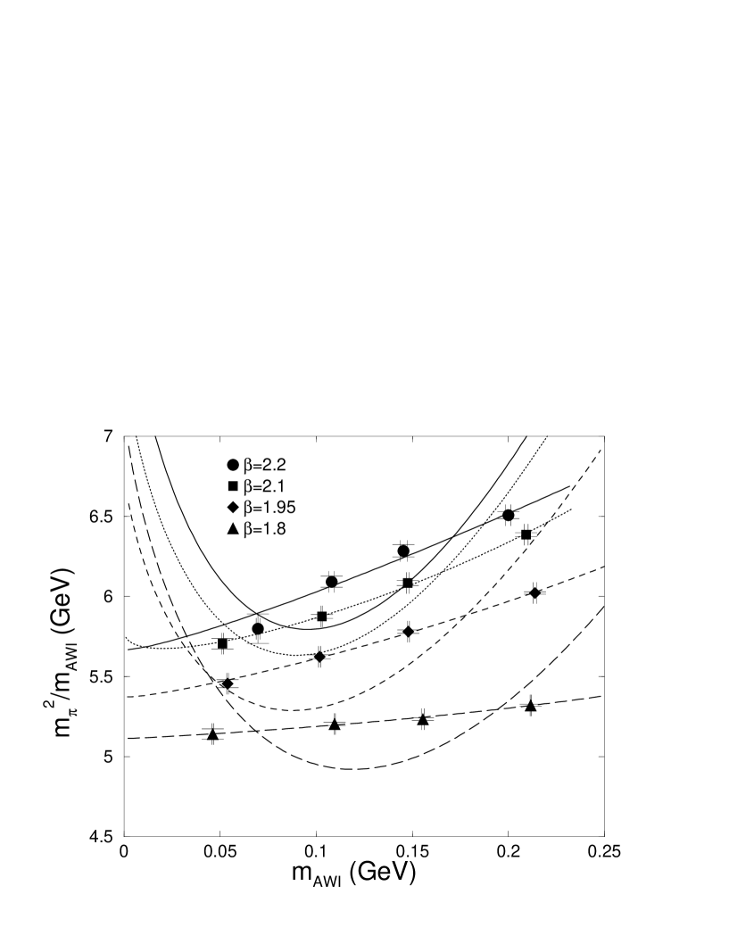
Figure 1: The WChPT fits for $m_{\pi}^{2}$ and $m_{\rm AWI}$ at each $\beta$. Results are shown for $m_{\pi}^{2}/m_{\rm AWI}$ as a function of $m_{\rm AWI}$. For comparison the standard ChPT fits ($w_{1}=w_{0}=0$) are also included.

Fig. 1 shows data and fits for $m_{\pi}^{2}/m_{\rm AWI}$ as a function of $m_{\rm AWI}$ at each $a$. For comparison, the results by the fit with the standard chiral perturbation theory ($w_{1}=w_{0}=0$) are also given. It is manifest that the WChPT fits perform much better than the ChPT fits. The parameters extracted from the fits are given in table 2. Note however that $\chi^{2}$/dof shown in the table has not been reliably estimated due to the correlation between $m_{\pi}^{2}$ and $m_{\rm AWI}$, which is not given in ref. cppacs .

In Fig. 2, $A$, $\Lambda$, $w_{1}a$, $w_{1}^{\rm AWI}a$ and $w_{0}a^{2}$ are plotted as a function of $a$, together with $K_{c}$ as a function of the bare gauge coupling constant $g^{2}$. While $A$, $\Lambda$ and $w_{1}a$ are too scattered to be fitted, $K_{c}$, $w_{0}a^{2}$ and $w_{1}^{\rm AWI}a$ may be fitted as

$$K_{c} = \frac{1}{8}\cdot\frac{1+d_{0}(K_{c})g^{2}+d_{1}(K_{c})g^{4}+d_{2}(K_{c})g^{6}}{1+(d_{0}(K_{c})-0.02945)g^{2}}$$ (58)

where 0.02945 is the 1-loop coefficientANTU and

$$w_{1}^{\rm AWI}a = d_{0}(w_{1})a,\qquad w_{0}a^{2}=d_{0}(w_{0})a^{2}.$$ (59)

Fit curves are also shown in Fig. 2, and the extracted parameters are given in the column (a) of table 3.

To determine $a$ dependences of $A$, $\Lambda$ and $w_{1}a$, we have fitted $m_{\pi}^{2}/m_{\rm AWI}$ as a function of both $m_{R}$ and $a$, using the following formula derived from eqs.(56,57) with $\Lambda_{\rm AWI}=\Lambda$:

$$\frac{m_{\pi}^{2}}{m_{\rm AWI}} = \frac{A}{A_{0}}\left[1+\frac{(A+\Delta w_{1}a)m_{R}}{32\pi^{2}f^{2}}\log\left(\frac{Am_{R}}{\Lambda^{2}}\right)\right]$$ (60)

where

$$A = d_{0}(A)\left(1+d_{1}(A)a+d_{2}(A)a^{2}\right),\qquad A_{0}=1+d_{0}(A_{0})a$$ (61)

$$\Lambda = d_{0}(\Lambda)\left(1+d_{1}(\Lambda)a^{2}\right),\qquad\Delta w_{1}=w_{1}-w_{1}^{\rm AWI}=d_{0}(\Delta w_{1})a.$$ (62)

No $\log m_{R}$ term is presented in eq.(60). Note however that $\log m_{\rm AWI}$ term appears again if we replace $m_{R}$ in the right-hand side of eq.(60) with $m_{\rm AWI}$, due to the presence of the $\log m_{R}$ term in eq.(57). With $K_{c}$ fixed to the values in table 2, the fit works well, as shown in Fig. 3, and the fitted parameters are given in the column (b) of table 3.

We roughly estimate the size of each parameter, $B_{1}$, $V_{2}$, $W_{1,2,3}$ from the continuum extrapolations of $A$, $w_{1}$, $w_{0}$ and $m_{c}$. Since we can not separate the $1/a$ contribution in $1/K_{c}$, however, $m_{c}$ can not be extracted. Therefore, we simply set $m_{c}=0$, giving that $W_{1}=2aW_{2}$; the leading contribution of $W_{1}$ vanishes. To reduce the number of the parameters further, we set $W_{0}=0$. Then extracting $B_{1}$, $W_{2}$ and $V_{2}$ as

$$B_{1} = f^{2}d_{0}(A)\equiv\left(\Lambda_{B_{1}}\right)^{3}$$ (63)

$$W_{2} = \frac{f^{2}d_{0}(w_{0})}{10}\equiv\left(\Lambda_{W_{2}}\right)^{6}$$ (64)

$$V_{2} = \frac{f^{2}d_{0}(w_{1})}{10}=\frac{f^{2}(d_{0}(w_{1}^{\rm AWI})+d_{0}(\Delta w_{1}))}{10}\equiv-\left(\Lambda_{V_{2}}\right)^{4},$$ (65)

we obtain $\Lambda_{B_{1}}=0.41$ GeV, $\Lambda_{W_{2}}=0.24$ GeV and $\Lambda_{V_{2}}=0.21$ GeV. These $\Lambda_{X}$ takes a reasonable value, $\Lambda_{X}=0.2\sim 0.4$ GeV. If $a\Lambda_{X}>m/\Lambda_{X}$, $O(a)$ terms become more important than $m_{R}$ terms. With $\Lambda_{X}=0.2\sim 0.4$ GeV, this condition at $a^{-1}$= 1 GeV or $a^{-1}$= 2 GeV corresponds to $m_{R}<40\sim 160$ MeV or $m_{R}<20\sim 80$ MeV, respectively.

III.3 Validity of the (W)ChPT

We now estimate the relative size size of the next-to-leading contribution to the leading contribution in the WChPT for $m_{\pi}^{2}$:

$$R(\mbox{WChPT}) = \frac{m_{R}(A+aw_{1})+a^{2}w_{0}}{32\pi^{2}f^{2}}\log\left(\frac{Am_{R}}{\Lambda^{2}}\right)$$ (66)

for the WChPT at finite $a$, where parameters $A$, $\Lambda$, $w_{1}$ and $w_{0}$ depend on $a$. We plot $R$(WChPT) in Fig. 4 at $a$(GeV^-1) =0, 0.44($\beta=2.2$), 0.55($\beta=2.1$), 0.79($\beta=1.95$) and 1.1($\beta=1.8$). While the 1-loop contribution takes reasonable values, 10% $\sim$ 30 % , at 0.1 GeV $<m_{R}<$ 0.2 GeV for all $a$, the contribution from $\log m_{R}$ in the WChPT diverges as $m_{R}\rightarrow 0$. This might invalidate the WChPT in the chiral limit. We will consider this problem in the next section.

IV Resummation of $\log m_{R}$ terms

As evident from the analysis in the previous subsection, $\log m_{R}$ contribution becomes larger and larger toward the chiral limit, so that we can not neglect “higher order” term such as $(\log m_{R})^{n}$ ($n=2,3,\cdots$). We must perform a resummation of $\log m_{R}$ term at all orders. Since it is possible in principle but difficult in practice to calculate $(\log m_{R})^{n}$ contribution at $n$-loop order, we derive resummed formulae from a different point of view.

As discussed in refs. aoki1 ; aoki2 ; aoki3 , the massless pion corresponds to the inverse of the divergent correlation length at the second order phase transition point. Since the effective theory which describes this phase transition is some 4 dimensional scalar(pion) theory with rather complicated interactions, the phase transition has the mean-field critical exponent with possible log-corrections. In particular the pion mass, the inverse of the correlation length, should behaves near the critical point as

$$m_{\pi}^{2} = Cm_{R}\left\{\log\left(\frac{m_{R}}{D}\right)\right\}^{\nu^{\prime}}+\cdots,$$ (67)

where $\cdots$ represent less singular contributions. If we expand

$$\left\{\log\left(\frac{m_{R}}{D}\right)\right\}^{\nu^{\prime}} = \left\{\log\left(\frac{\Lambda_{0}^{2}}{AD}\right)+\log\left(\frac{Am_{R}}{\Lambda_{0}^{2}}\right)\right\}^{\nu^{\prime}}=X^{\nu^{\prime}}\sum_{n=0}^{\infty}\frac{\nu^{\prime}!}{(\nu^{\prime}-n)!n!}\left(\frac{Y}{X}\right)^{n}$$ (68)

$$= X^{\nu^{\prime}}\left(1+\nu^{\prime}\frac{Y}{X}+\cdots\right)$$

where

$$X = \log\left(\frac{\Lambda_{0}^{2}}{AD}\right)$$ (69)

$$Y = \log\left(\frac{Am_{R}}{\Lambda_{0}^{2}}\right),$$ (70)

the formula at the next-to-leading order in WChPT, eq.(56), is recovered, with the identification that

$$\frac{\nu^{\prime}}{X} = \frac{a^{2}w_{0}}{32\pi^{2}f^{2}},\qquad CX^{\nu^{\prime}}=A.$$ (71)

To determine $\nu^{\prime}$ and $X$ separately, the explicit calculation in the WChPT at 2-loop or more orders is necessary. This will be considered in future investigations.

We have finally obtained the following resummed formulae for $m_{\pi}^{2}$ and $m_{\rm AWI}$:

$$m_{\pi}^{2} = Am_{R}\left\{\log\left(\frac{m_{R}}{\Lambda_{0}}\right)\right\}^{\frac{a^{2}w_{0}}{32\pi^{2}f^{2}}}\left[1+\frac{m_{R}A+m_{R}aw_{1}}{32\pi^{2}f^{2}}\log\left(\frac{Am_{R}}{\Lambda^{2}}\right)\right]$$ (72)

$$m_{\rm AWI} = A_{0}m_{R}\left\{\log\left(\frac{m_{R}}{\Lambda_{0}}\right)\right\}^{\frac{a^{2}w_{0}}{32\pi^{2}f^{2}}}\left[1+\frac{m_{R}aw_{1}^{\rm AWI}}{32\pi^{2}f^{2}}\log\left(\frac{Am_{R}}{\Lambda_{\rm AWI}^{2}}\right)\right],$$ (73)

where $A$, $\Lambda_{0}$ and $\omega_{0}$ may be different from those in eqs.(56,57). It is better to use these formulae instead of the previous ones, eqs.(56,57), in future investigations. Eq.(60) remains the same.

As a trial, we use these formulae with $A_{0}=1$, $\Lambda_{\rm AWI}=\Lambda$ and $\Lambda_{0}$=1 GeV, in order to fit $m_{\pi}^{2}$ and $m_{\rm AWI}$ simultaneously, at each $a$. The quality of the fit is as good as the previous one, and the fitting parameters are compiled in the end of table 2. In addition, the next-to-leading contribution, the second term in eq.(73), vanishes toward $m_{R}=0$ as shown in Fig. 4, where $R$(WChPT) in the previous subsection, which is now modified as

$$R(\mbox{WChPT, resum}) = \frac{m_{R}A+m_{R}aw_{1}}{32\pi^{2}f^{2}}\log\left(\frac{Am_{R}}{\Lambda^{2}}\right),$$ (74)

are plotted at $\beta=$ 1.8, 1.95, 2.1 and 2.2 .

V Conclusions and Discussions

In this paper we have derived the effective chiral Lagrangian which includes the $a^{2}$ effect of the Wilson-type quark action in the case of the $N_{f}=2$ degenerate quarks. Using this effective Lagrangian the quark mass($m_{R}$) dependences of $m_{\pi}^{2}$, $m_{\rm AWI}$ and $f_{\pi}$ have been calculated at the 1-loop level. We then have simultaneously fitted $m_{\pi}^{2}$ and $m_{\rm AWI}$, obtained by the CP-PACS collaboration for $N_{f}=2$ full QCD simulations, using the WChPT formula, and have found that the data are consistently described. We have attempted the continuum extrapolation of the WChPT formula.

Comparing to the standard ChPT, several distinct features such as the additive mass renormalization, $O(a)$ corrections to the chiral log($m_{R}\log m_{R}$) term, a more singular term($\log m_{R}$) generated by $O(a^{2})$ contributions and the presence of both $m_{R}\log m_{R}$ and $\log m_{R}$ terms in $m_{\rm AWI}$, leads to the success for the WChPT formula to describe the CP-PACS data. Although an ambiguity for the definition of $K_{c}$ caused by the additive mass renormalization can be avoided by the use of $m_{\rm AWI}$, the last feature, the existence of both $m_{R}\log m_{R}$ and $\log m_{R}$ terms in $m_{\rm AWI}$, makes the WChPT formula different from the ChPT’s. The large $O(a)$ correction to $m_{R}\log m_{R}$ term plays an essential role to describe the actual data, though more or less others have some contributions. We have also derived the formula after resumming $\log m_{R}$ terms, using the fact that the mean-field critical exponent receives the log-correction.

Because of the limitation of available data, our WChPT analysis is far from complete. Therefore it is important to refine the analysis by taking the correlation between $m_{\pi}^{2}$ and $m_{\rm AWI}$ into account and including $f_{\pi}$ data in the simultaneous fit, in order to establish the validity of the WChPT. Reanalyses of other full QCD data have to be done of course. It is also urgent to derive the WChPT formula for other casesBRS such as the quench/partially quench cases, the $N_{f}=3$ non-degenerate case, vector mesons and baryons, heavy-light mesons.

Once the validity of the WChPT to describe lattice QCD data is established, instead of thinking that the quark masses in the current full QCD simulations are too heavy for the ChPT to apply, we may say that some (but not all) of lattice data are well described by the (Wilson) chiral perturbation theory, by which errors associated with the chiral extrapolation may be well controlled ks .

Table 1: Parameters of $N_{f}=2$ full QCD simulations by the CP-PACS collaboration cppacs . The scale $a$ is fixed by $m_{\rho}=$ 768.4 MeV.

$\beta$	$L^{3}\times T$	$c_{\rm SW}$	$a$ [fm]	$a^{-1}$ [GeV]	$La$ [fm]	$m_{\pi}/m_{\rho}$
1.80	$12^{3}\times 24$	1.60	0.2150(22)	0.9178(94)	2.580(26)	0.55$\sim$ 0.81
1.95	$16^{3}\times 32$	1.53	0.1555(17)	1.269(14)	2.489(27)	0.58$\sim$ 0.80
2.10	$24^{3}\times 48$	1.47	0.1076(13)	1.834(22)	2.583(31)	0.58$\sim$ 0.81
2.20	$24^{3}\times 48$	1.44	0.0865(33)	2.281(87)	2.076(79)	0.63$\sim$ 0.80

Table 2: Parameters of the WChPT fit at each $\beta$.

$\beta$	$K_{c}$	$A$[GeV]	$\Lambda$ [GeV]	$w_{1}a$[GeV]	$w_{0}a^{2}$[GeV2]	$w_{1}^{\rm AWI}a$ [GeV]	$\chi^{2}$/dof
1.80	0.147761(15)	5.114(28)	0.079(19)	-5.525(64)	0.206(22)	-0.560(74)	0.3
1.95	0.142160(19)	5.377(33)	0.193(51)	-5.162(74)	0.241(42)	-0.457(118)	0.3
2.10	0.139110(12)	5.807(14)	0.694(20)	-5.24(18)	0.417(50)	-1.15(27)	0.2
2.20	0.137691(23)	5.669(71)	0.128(88)	-5.15(20)	0.039(16)	-0.22(39)	0.7
	resummed WChPT
1.8	0.147562(15)	5.111(29)	0.067(12)	-4.862(46)	0.787(21)	0.124(15)	1.5
1.95	0.142009(7)	5.366(23)	0.132(15)	-4.538(52)	0.624(18)	0.310(32)	0.3
2.1	0.138959(13)	5.535(47)	0.131(71)	-4.79(14)	0.280(37)	0.181(49)	1.2
2.2	0.137657(36)	5.789(106)	0.391(82)	-4.63(12)	0.201(95)	0.195(96)	0.8

Table 3: Continuum extrapolation of the WChPT fit parameters. (a) $m_{\pi}^{2}$ and $m_{\rm AWI}$ are fitted as a function of $m_{R}$ at each $a$. Then parameters are fitted as a function of $a$. (b) $m_{\pi}^{2}/m_{\rm AWI}$ are fitted as a function of $m_{R}$ and $a$

(a)					(b)  $\chi^{2}$/dof=1.3
$X$	$d_{0}(X)$	$d_{1}(X)$	$d_{2}(X)$	$\chi^{2}$/dof	$X$	$d_{0}(X)$	$d_{1}(X)$	$d_{2}(X)$
$K_{c}$	-0.2127(10)	-0.008300(55)	0.000787(31)	3.6	$A$	8.087(97)	-1.002(29)	0.2672(29)
$w_{0}$	0.202(17)	0	0	20	$\Lambda$	1.196(35)	-0.8404(58)	0
$w_{1}^{\rm AWI}$	-0.549(61)	0	0	3.4	$\Delta w_{1}$	-1.62(25)	0	0
					$A_{0}$	-0.590(47)	0	0

Figure 2: The fit parameters as a function of $a$ or $g^{2}$.

Figure 3: The WChPT fits for $m_{\pi}^{2}/m_{\rm AWI}$ as a function of $m_{R}$ and $a$. Results are shown for $m_{\pi}^{2}/m_{\rm AWI}$ as a function of $m_{R}$.

Figure 4: Left: The relative size of the next-to-leading contribution to the leading one in the WChPT as a function of the quark mass $m_{R}$ at $\beta$=1.8,1.95,2.1 and 2.2, together with the one in the continuum limit (ChPT). Right: Same quantities in the resummed WChPT.

References

- (1) S. Weinberg, Physica 96A (1979) 327; J. Gasser and H. Leutwyler, Ann. Phys. 158 (1984) 142; Nucl. Phys. B250 (1985) 465; 517 ;539.
- (2) For the recent discussion, see C. Bernard et al., “Panel discussion on chiral extrapolation of physical observables”, hep-lat/0209086.
- (3) S. R. Sharpe and R. Singleton Jr., Phys. Rev. D58 (1998) 074501.
- (4) G. Rupak and N. Shoresh, Phys. Rev. D66 (2002) 054503
- (5) S. Aoki, Phys. Rev. D30 (1984) 2653; Phys. Rev. Lett. 57 (1986) 3136; Nucl. Phys. B314 (1989) 79; Prog. Theor. Phys. 122 (1996) 179.
- (6) S. Aoki and A. Gocksch, Phys. Lett. B231 (1989) 449; 243 (1990) 409; Phys. Rev. F45 (1992) 3845.
- (7) S. Aoki, A. Ukawa and T. Umemura, Phys. Rev. Lett. 76 (1996) 873; Nucl. Phys. B(Proc.Suppl.) 47 (1996) 511; S. Aoki, T. Kaneda, A. Ukawa and T. Umemura, Nucl. Phys. B(Proc.Suppl.) 53 (1997) 438; S. Aoki, T. Kaneda, and A. Ukawa, Phys. Rev. D56 (1997) 1808; S. Aoki, Nucl. Phys. B(Proc.Suppl.) 60A (1998) 206.
- (8) CP-PACS Collaboration (A. Ali Khan et al.), Phys. Rev. Lett. 85 (2000) 4674-4677; Erratum-ibid. 90 (2003) 029902; Phys. Rev. D65 (2002) 054505; Erratum-ibid. D67 (2003) 059901.
- (9) K. Symanzik, Nucl. Phys. B226 (1983) 187; 205.
- (10) B. Sheikholeslami and R. Wohlert, Nucl. Phys. B259 (1985) 572.
- (11) S. Aoki, K. Nagai, Y. Taniguchi and A. Ukawa, Phys. Rev. D58 (1998) 074505.
- (12) After completing this work, there appears a related work, in which contributions in the ChPT are considered in general cases. O. Baer, G. Rupak and N. Shoresh, “Chiral perturbation theory at for lattice QCD”, hep-lat/0306021.
- (13) The similar attempts have already been made for the case of the staggered fermions. C. Bernard, Phys. Rev. D65 (2002) 054031; C. Aubin and C. Bernard, hep-lat/0304014; hep-lat/0306026.