Pseudoscalar Decay Constants in Staggered Chiral Perturbation Theory

Abstract

In a continuation of an ongoing program, we use staggered chiral perturbation theory to calculate the one-loop chiral logarithms and analytic terms in the pseudoscalar meson leptonic decay constants, $f_{\pi^{+}_{5}}$ and $f_{K^{+}_{5}}$. We consider the partially quenched, “full QCD” (with three dynamical flavors), and quenched cases.

I Introduction

Simulations with staggered (Kogut-Susskind, KS) fermions are very fast relative to other available approaches, making possible simulations of QCD that include the effects of light sea quarks CHIRAL_PANEL_2001 . However, with currently practical lattice spacings (e.g., MILC simulations PETER_PRL ; IMP_SCALING ; IMP_SCALING2 ; MILC_SPECTRUM ; FB_LAT02 at $a\approx 0.09-0.13\ \rm fm$) taste violations are not negligible. Thus fits to such lattice data should take into account the taste-violating effects; indeed, if such effects are not taken into account, the speed advantage of KS fermions may be offset by the size of the systematic errors. The taste-violating effects can be calculated in a systematic way using staggered chiral perturbation theory (S$\chi$PT).

In Ref. AUBIN , we formulate S$\chi$PT for the physical case of multiple flavors. S$\chi$PT is then used to calculate the one-loop chiral logarithms in the pion and kaon masses. Here, we continue the program of Ref. AUBIN and compute $f_{\pi^{+}_{5}}$ and $f_{K^{+}_{5}}$, the $\pi^{+}$ and $K^{+}$ leptonic decay constants for the Goldstone mesons, to one loop. As we have laid most of the necessary groundwork already, we will merely state what is necessary for this present work and refer the reader to Ref. AUBIN for the details common to both calculations. As in the calculation of the $\pi^{+}$ and $K^{+}$ masses, we perform our calculation using three dynamical KS-flavors (each with four tastes), which we call the $4\!+\!4\!+\!4$ theory, and later adjust the result by hand using a quark flow technique AUBIN ; SHARPE_QCHPT to a $1\!+\!1\!+\!1$ theory (three flavors each with a single taste).

The outline of this paper is as follows: In Sec. II, we write down the S$\chi$PT Lagrangian for three dynamical flavors. We then calculate, in Sec. III, the one-loop chiral logarithms which contribute to the flavor-nonsinglet Goldstone meson decay constant in the partially quenched case. Here we keep three dynamical flavors but add two additional quenched flavors as valence quarks, which in the general case have distinct masses from the dynamical (sea) quarks. The transition to a $1\!+\!1\!+\!1$ theory is then made. There are only a few differences in this procedure from that of Ref. AUBIN . We also give the results in the fully quenched case. The full next-to-leading order (NLO) results, including the analytic terms, are presented in Sec. IV for various relevant cases. We conclude with some comments in Sec. V. An Appendix gives technical details about the evaluation of the one-loop integrals that arise in Sec. III.

II The Lee-Sharpe Lagrangian for 3 flavors

The starting point for S$\chi$PT is the Lee-Sharpe Lagrangian LEE_SHARPE generalized to multiple flavors. In Ref. AUBIN we examined a general $n$-flavor theory and later specialized to $n=3$. Here we take $n=3$ from the beginning. For 3 KS flavors, $\Sigma=\exp(i\Phi/f)$ is a $12\times 12$ matrix, with $\Phi$ given by:

$$\Phi=\left(\begin{array}[]{ccc}U&\pi^{+}&K^{+}\\ \pi^{-}&D&K^{0}\\ K^{-}&\bar{K^{0}}&S\end{array}\right),$$ (4)

where $U=\sum_{a=1}^{16}U_{a}T_{a}$ (and similarly for $\pi^{+}$, $K^{+}$, …), with

$$T_{a}=\{\xi_{5},i\xi_{\mu 5},i\xi_{\mu\nu},\xi_{\mu},\xi_{I}\}.$$ (5)

We use the Euclidean gamma matrices $\xi_{\mu}$, with $\xi_{\mu\nu}\equiv\xi_{\mu}\xi_{\nu}$ ($\mu<\nu$ in Eq. (5)), $\xi_{\mu 5}\equiv\xi_{\mu}\xi_{5}$, and $\xi_{I}\equiv I$ is the $4\times 4$ identity matrix. The field $\Sigma$ transforms under $SU(12)_{L}\times SU(12)_{R}$ as $\Sigma\rightarrow L\Sigma R^{\dagger}$. The component fields of the diagonal (flavor-neutral) elements ($U_{a}$, $D_{a}$, and $S_{a}$) are real; the other, charged, fields ($\pi^{+}_{a}$, $K^{0}_{a}$, etc.) are complex, so that $\Phi$ is Hermitian. The mass matrix is given by the $12\times 12$ matrix

$$\mathcal{M}=\left(\begin{array}[]{ccc}m_{u}I&0&0\\ 0&m_{d}I&0\\ 0&0&m_{s}I\end{array}\right)\ .$$ (9)

Our (Euclidean) Lagrangian is:

$$\mathcal{L} = \frac{f^{2}}{8}\textrm{Tr}(\partial_{\mu}\Sigma\partial_{\mu}\Sigma^{\dagger})-\frac{1}{4}\mu f^{2}\textrm{Tr}(\mathcal{M}\Sigma+\mathcal{M}\Sigma^{\dagger})+\frac{2m_{0}^{2}}{3}(U_{I}+D_{I}+S_{I})^{2}+a^{2}\mathcal{V},$$ (10)

where $\mu$ is a constant with units of mass, Tr is the full $12\times 12$ trace, and $\mathcal{V}=\mathcal{U}+\mathcal{U}\,^{\prime}$ is the taste-symmetry breaking potential. The $\mathcal{U}$ term is given in Ref. AUBIN ; it is not needed explicitly here. For $\mathcal{U}\,^{\prime}$, we have

$$-\mathcal{U}\,^{\prime} = C_{2V}\frac{1}{4}\sum_{\nu}[\textrm{Tr}(\xi^{(3)}_{\nu}\Sigma)\textrm{Tr}(\xi^{(3)}_{\nu}\Sigma)+h.c.]$$ (11)

$$+C_{2A}\frac{1}{4}\sum_{\nu}[\textrm{Tr}(\xi^{(3)}_{\nu 5}\Sigma)\textrm{Tr}(\xi^{(3)}_{5\nu}\Sigma)+h.c.]$$

$$+C_{5V}\frac{1}{2}\sum_{\nu}[\textrm{Tr}(\xi^{(3)}_{\nu}\Sigma)\textrm{Tr}(\xi^{(3)}_{\nu}\Sigma^{\dagger})]$$

$$+C_{5A}\frac{1}{2}\sum_{\nu}[\textrm{Tr}(\xi^{(3)}_{\nu 5}\Sigma)\textrm{Tr}(\xi^{(3)}_{5\nu}\Sigma^{\dagger})],$$

where the $\xi^{(3)}_{B}$ are block-diagonal $12\times 12$ matrices:

$$\xi^{(3)}_{B}=\left(\matrix{\xi_{B}&0&0\cr 0&\xi_{B}&0\cr 0&0&\xi_{B}\cr}\right)\ ,$$ (12)

with $\xi_{B}$ the $4\times 4$ objects, and $B\in\{5,\mu,\mu\nu\ (\mu<\nu),\mu 5,I\}$.

As seen in Ref. AUBIN , $\mathcal{U}\,^{\prime}$ generates two-point vertices at $\mathcal{O}(a^{2})$ (shown in Fig. 1) that mix flavor-neutral particles of vector and axial tastes. In addition, flavor-neutral, taste-singlet particles are mixed by the $m_{0}^{2}$ term in Eq. (10), which results from the anomaly. In all three cases (taste vector, axial vector, and singlet), we have a term in the Lagrangian of the form $(\delta^{\prime}/2)(U+D+S)^{2}$, where

$$\delta^{\prime}=\cases{a^{2}\delta^{\prime}_{V},&taste-vector;\cr a^{2}\delta^{\prime}_{A},&taste-axial;\cr 4m_{0}^{2}/3,&taste-singlet.\cr}$$ (13)

Expressions for $\delta^{\prime}_{V}$ and $\delta^{\prime}_{A}$ in terms of the coefficients of $\mathcal{U}\,^{\prime}$ are given in Ref. AUBIN . These mixings require us to diagonalize the full mass matrix in each of the three channels. We write the propagator for the vectors as:

$$G_{V} = G_{0,V}+\mathcal{D}^{V}\ .$$ (14)

$\mathcal{D}^{V}$ is the part of the taste-vector flavor-neutral propagator that is disconnected at the quark level (i.e., Fig. 1 plus iterations of intermediate sea quark loops). Explicitly, we have AUBIN :

$$\mathcal{D}^{V}_{MN} = -a^{2}\delta^{\prime}_{V}\frac{(q^{2}+m_{U_{V}}^{2})(q^{2}+m_{D_{V}}^{2})(q^{2}+m_{S_{V}}^{2})}{(q^{2}+m_{M_{V}}^{2})(q^{2}+m_{N_{V}}^{2})(q^{2}+m_{\pi^{0}_{V}}^{2})(q^{2}+m_{\eta_{V}}^{2})(q^{2}+m_{\eta^{\prime}_{V}}^{2})}\ .$$ (15)

Here, $m_{\pi^{0}_{V}}^{2}$, $m_{\eta_{V}}^{2}$ and $m_{\eta^{\prime}_{V}}^{2}$ are the eigenvalues of the full mass-squared matrix (i.e., the poles of $G_{V}$). We emphasize that Eq. (15) remains valid in the $n=3$ partially quenched case. The external mesons $M$ and $N$ may be any flavor-neutral states, made from either sea quarks or valence quarks.

In the quenched case $\mathcal{D}^{V}_{MN}$ is simply

$$\mathcal{D}^{V,\rm quench}_{MN}=-a^{2}\delta^{\prime}_{V}\frac{1}{(q^{2}+m_{M_{V}}^{2})(q^{2}+m_{N_{V}}^{2})}\ .$$ (16)

Equations (14) through (16) apply explicitly to the taste-vector channel; to get the result in the taste-axial (taste-singlet) channel, just let $V\to A$ ($V\to I$ and $a^{2}\delta^{\prime}_{V}\rightarrow 4m^{2}_{0}/3$). In the quenched case we cannot take $m_{0}\to\infty$, and must include additional $\eta^{\prime}_{I}$-dependent terms in the Lagrangian, resulting in the replacement $m_{0}^{2}\to m_{0}^{2}+\alpha q^{2}$ in the singlet form of Eq. (16) AUBIN ; CBMG_QCHPT .

III One loop decay constant for 4+4+4 dynamical flavors

We calculate the pion decay constant in a partially quenched theory. Full theory results are easily obtained by taking appropriate limits. There are three sea quarks ($u$, $d$ and $s$) and two valence quarks ($x$ and $y$). The pion of interest is the $P^{+}_{5}$, a Goldstone pion which is composed of an $x\bar{y}$ pair of quarks.

The $P^{+}_{5}$ decay constant is defined by the matrix element:

$$\left\langle 0\left|j_{\mu 5}^{P^{+}_{5}}\right|P^{+}_{5}(p)\right\rangle=-if_{P^{+}_{5}}p_{\mu}\ ,$$ (17)

where $j_{\mu 5}^{P^{+}_{5}}$ is the axial current corresponding to ${P^{+}_{5}}$. With this normalization, $f_{\pi}\approx 131\ {\rm Me\!V}$. In terms of $\Sigma$, we can write the axial current as

$$j_{\mu 5}^{P^{+}_{5}} = \frac{-if^{2}}{8}\textrm{Tr}\left[\xi^{(3)}_{5}\mathcal{P}^{P^{+}}\left(\partial_{\mu}\Sigma\Sigma^{\dagger}+\Sigma^{\dagger}\partial_{\mu}\Sigma\right)\right]\ .$$ (18)

Here $\mathcal{P}^{P^{+}}$ projects out the $4\times 4$ block with appropriate flavor: If we make $x$ and $y$ the last two flavors of $\Sigma$, then $\mathcal{P}^{P^{+}}_{ij}=\delta_{i5}\delta_{j4}$, where $i,j$ are flavor indices.

At one loop, the decay constant has the form

$$f_{P^{+}_{5}}=f\left(1+\frac{1}{16\pi^{2}f^{2}}\delta\!f_{P^{+}_{5}}\right)\ .$$ (19)

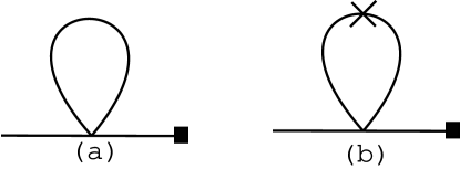
Figure 2: The S$\chi$PT diagrams contributing to the pion decay constant, coming from wave-function renormalization. The box represents the the axial current. (a) is the connected piece, where the propagator in the loop contains no two-point vertex insertions. (b) subsumes the graphs which have disconnected insertions within the loop. The cross represents one or more insertions of the $\delta^{\prime}$ vertex, with $\delta^{\prime}$ given in Eq. (13).

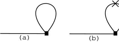
Figure 3: Same as Fig. 2, but these contributions to the decay constant are from axial current corrections.

There are two contributions to $\delta\!f_{P^{+}_{5}}$, which we call $\delta\!f^{\rm Z}_{P^{+}_{5}}$ and $\delta\!f^{\rm current}_{P^{+}_{5}}$. They are shown in Figs. 2 and 3, respectively. The contribution $\delta\!f^{\rm Z}_{P^{+}_{5}}$ is merely wavefunction renormalization. We have:

$$\delta\!f^{\rm Z}_{P^{+}_{5}}=\frac{1}{2}\delta\!Z_{P^{+}_{5}}\equiv-\frac{16\pi^{2}f^{2}}{2}\;{d\Sigma(p^{2})\over dp^{2}}\ .$$ (20)

The self-energy, $\Sigma(p^{2})$, has already been calculated in Ref. AUBIN . The wavefunction renormalization arises only from the vertex generated by the kinetic energy term in Eq. (10), since derivatives on the external lines are necessary to generate $p^{2}$ dependence in a tadpole diagram. The factor of $1/2$ in Eq. (20) is due to the fact that this diagram is multiplied by $\sqrt{Z}=\sqrt{1+\delta\!Z}\approx 1+\frac{1}{2}\delta\!Z$.

The contribution $\delta\!f^{\rm current}_{P^{+}_{5}}$ is the current correction. It arises from the expansion of Eq. (18) to cubic order in $\Phi$. Performing this expansion, it is easy to see that the wavefunction and current correction terms are proportional to each other: $\delta\!f^{\rm current}_{P^{+}_{5}}=-4\delta\!f^{\rm Z}_{P^{+}_{5}}$. This fact, noted also in SHARPE_QCHPT , is perhaps not surprising, since the form of the axial current, Eq. (18), is determined through Noether’s theorem only by the kinetic energy part of the Lagrangian. From Eq. (20), we then have

$$\delta\!f_{P^{+}_{5}} = \delta\!f^{\rm Z}_{P^{+}_{5}}+\delta\!f^{\rm current}_{P^{+}_{5}}=-\frac{3}{2}\delta\!Z_{P^{+}_{5}}\ .$$ (21)

Using intermediate expressions for $\Sigma(p^{2})$ from AUBIN , the one-loop result is

$$\delta\!f_{P^{+}_{5}} = -\frac{1}{8}\int\frac{d^{4}q}{\pi^{2}}\Biggl{[}\sum_{Q,B}\biggl{(}\frac{1}{q^{2}+m^{2}_{Q_{B}}}\biggr{)}+\mathcal{D}^{I}_{XX}-2\mathcal{D}^{I}_{XY}+\mathcal{D}^{I}_{YY}$$ (22)

$$+4\mathcal{D}^{V}_{XX}+8\mathcal{D}^{V}_{XY}+4\mathcal{D}^{V}_{YY}+4\mathcal{D}^{A}_{XX}+8\mathcal{D}^{A}_{XY}+4\mathcal{D}^{A}_{YY}\Biggr{]}\ .$$

Here, $Q$ runs over the six mesons formed from one valence and one sea quark (i.e., the $xu$, $xd$, $xs$, $yu$, $yd$, and $ys$ mesons). As before, $B$ takes on the 16 values $\{5,\mu,\mu\nu(\mu<\nu),\mu 5,I\}$. We have already included the factor of 4 that comes from summing over the degenerate vector and axial contributions in the $\mathcal{D}^{V}$ and $\mathcal{D}^{A}$ terms. Despite the fact that the only 4-point vertices contributing to this expression come from the kinetic energy term, the result is more complicated than that for the mass renormalization AUBIN because there are no cancellations here (either accidental or required by symmetry).

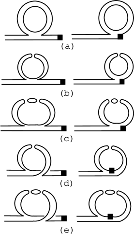
Figure 4: The quark level diagrams that contribute to the one-loop pion decay constant. The box represents an insertion of the axial current. The diagrams on the left correspond to the wavefunction renormalization while those on the right correspond to the current corrections.

The first term Eq. (22) (the sum over $Q$ and $B$) comes from the wave function renormalization and current correction diagrams shown in Fig. 4(a), which involve a single virtual quark loop. The diagrams arise from the vertices in Fig. 5(a), respectively, where $i$ is summed over the sea quarks only. In this case, the propagator in the loop must be connected since the loop meson is not flavor-neutral.

The vertices in Fig. 5(a) also produce diagrams with disconnected loop propagators, Fig. 4(b) and (c), when $i=y$ (or $i=x$ in the $y\leftrightarrow x$ version of Fig. 5(a)). These diagrams give rise to the $\mathcal{D}_{YY}$ and $\mathcal{D}_{XX}$ terms in Eq. (22).

Finally, the vertices in Fig. 5(b) generate the diagrams Fig. 4(d) and (e). The $\mathcal{D}_{XY}$ terms in Eq. (22) come from these diagrams. For more discussion of how to identify quark flow diagrams with the S$\chi$PT contributions, see Ref. AUBIN .

We can write down the quenched result by (1) eliminating the term summed over $Q$ and $B$, which arises from virtual quark loops (diagrams Fig. 4(a)), and (2) replacing of $\mathcal{D}\to\mathcal{D}^{\rm quench}$ for $\mathcal{D}^{V}$, $\mathcal{D}^{A}$, and $\mathcal{D}^{I}$. These replacements eliminate diagrams Fig. 4(c) and (e).

In the partially quenched case, when the $x$ or $y$ quark mass is different from all sea quark masses, there are double poles in Eq. (22) coming from the $\mathcal{D}_{XX}$ or $\mathcal{D}_{YY}$ terms. This is different from the mass renormalization result, where double poles do not arise unless $m_{x}=m_{y}$ and this mass is different from all sea quark masses, a case we did not treat in detail in Ref. AUBIN . In order to write down explicit results for partial quenching here, we must therefore expand on the notation of Ref. AUBIN . Below we will use the notation defined in the Appendix, where we explain the techniques we use to evaluate the integrals.

Before performing the momentum integrals, we now make the transition from the $4\!+\!4\!+\!4$ case to the $1\!+\!1\!+\!1$ case. This is easily accomplished since we have already determined the separate contributions from diagrams in Fig. 4 with various numbers of sea quark loops. Those diagrams with a connected propagator in the loop, Fig. 4(a), have a single sea quark loop and simply must be divided by 4.

The remaining diagrams have the same form as those treated in Ref. AUBIN , so we just briefly review the procedure. Diagrams (b) and (d) in Fig. 4 have no sea quark loops and are unaffected by the transition to the $1\!+\!1\!+\!1$ case. These diagrams have a single factor of $\delta^{\prime}$ coming from the overall coefficient of the disconnected propagator $\mathcal{D}$ in Eq. (15). Each sea quark loop added on to diagrams (b) and (d), as in (c) and (e), comes with an additional factor of $\delta^{\prime}$. Therefore, we must merely make the replacement $\delta^{\prime}\to\delta^{\prime}/4$ in all but the overall factors of $\delta^{\prime}$. This is easily accomplished by letting $\delta^{\prime}\to\delta^{\prime}/4$ in the computation of the full mass eigenstates (i.e., $m^{2}_{\pi_{V}^{0}}$, $m^{2}_{\eta_{V}}$ and $m^{2}_{\eta^{\prime}_{V}}$ in Eq. (15)), but not in the overall coefficient of $\mathcal{D}$.

After making the transition to the $1\!+\!1\!+\!1$ case, taking the $m_{0}\to\infty$ limit (with $m^{2}_{\eta^{\prime}_{I}}\sim m_{0}^{2}$), and using Eq. (37) through Eq. (46) to perform the momentum integrals, we have

$$\delta\!f_{P^{+}_{5}} \to-\frac{1}{32}\sum_{Q,B}\ell\left(m^{2}_{Q_{B}}\right)+\frac{1}{6}\Biggl{(}R^{[3,3]}_{X_{I}}(\{\mathcal{M}^{(1)}_{X_{I}}\})\tilde{\ell}(m^{2}_{X_{I}})+R^{[3,3]}_{Y_{I}}(\{\mathcal{M}^{(1)}_{Y_{I}}\})\tilde{\ell}(m^{2}_{Y_{I}})$$ (23)

$$+\sum_{j_{I}}D^{[3,3]}_{j_{I},X_{I}}(\{\mathcal{M}^{(1)}_{X_{I}}\})\ell(m^{2}_{j_{I}})+\sum_{j_{I}}D^{[3,3]}_{j_{I},Y_{I}}(\{\mathcal{M}^{(1)}_{Y_{I}}\})\ell(m^{2}_{j_{I}})$$

$$-2\sum_{j_{I}}R^{[4,3]}_{j_{I}}(\{\mathcal{M}^{(2)}_{I}\})\ell(m^{2}_{j_{I}})\Biggr{)}+\frac{1}{2}a^{2}\delta^{\prime}_{V}\Biggl{[}R^{[4,3]}_{X_{V}}(\{\mathcal{M}^{(3)}_{X_{V}}\})\tilde{\ell}(m^{2}_{X_{V}})$$

$$+R^{[4,3]}_{Y_{V}}(\{\mathcal{M}^{(3)}_{Y_{V}}\})\tilde{\ell}(m^{2}_{Y_{V}})+\sum_{j_{V}}D^{[4,3]}_{j_{V},X_{V}}(\{\mathcal{M}^{(3)}_{X_{V}}\})\ell(m^{2}_{j_{V}})$$

$$+\sum_{j_{V}}D^{[4,3]}_{j_{V},Y_{V}}(\{\mathcal{M}^{(3)}_{Y_{V}}\})\ell(m^{2}_{j_{V}})+2\sum_{j_{V}}R^{[5,3]}_{j_{V}}(\{\mathcal{M}^{(4)}_{V}\})\ell(m^{2}_{j_{V}})\Biggr{]}+\Bigl{[}V\to A\Bigr{]}\ ,$$

where $Q$ and $B$ have the same meaning as in Eq. (22), the chiral logarithms $\ell(m^{2})$ are defined in Eqs. (49) and (51) for infinite and finite spatial volume, respectively, and the $R$s and $D$s are residues defined in Eqs. (39) and (42). The arrow signifies that we are only keeping the chiral logarithm terms in this expression. We have defined the sets of masses in the residues:

$$\{\mathcal{M}^{(1)}_{Z}\} \equiv \{m_{\pi^{0}},m_{\eta},m_{Z}\}\ ,$$

$$\{\mathcal{M}^{(2)}\} \equiv \{m_{\pi^{0}},m_{\eta},m_{X},m_{Y}\}\ ,$$

$$\{\mathcal{M}^{(3)}_{Z}\} \equiv \{m_{\pi^{0}},m_{\eta},m_{\eta^{\prime}},m_{Z}\}\ ,$$

$$\{\mathcal{M}^{(4)}\} \equiv \{m_{\pi^{0}},m_{\eta},m_{\eta^{\prime}},m_{X},m_{Y}\}\ ,$$ (24)

where $Z$ can be either $X$ or $Y$, and we show the taste labels explicitly in Eq. (23). We do not include the numerator masses in the argument of the residues, as they are the same for each case:

$$\{\mu\}=\{m_{U},m_{D},m_{S}\}\ ,$$ (25)

with appropriate taste subscripts. The sums over $j_{I}$, $j_{V}$, and $j_{A}$ run over the set of masses included as the argument of the residues in each sum.

The values of $m^{2}_{\pi^{0}}$, $m^{2}_{\eta}$ and $m^{2}_{\eta^{\prime}}$ in each taste channel in Eq. (23) are the eigenvalues of the full mass matrix

$$\left(\matrix{m^{2}_{U}+\delta^{\prime}/4&\delta^{\prime}/4&\delta^{\prime}/4\cr\delta^{\prime}/4&m^{2}_{D}+\delta^{\prime}/4&\delta^{\prime}/4\cr\delta^{\prime}/4&\delta^{\prime}/4&m^{2}_{S}+\delta^{\prime}/4\cr}\right)\ ,$$ (26)

where $\delta^{\prime}$ is given by Eq. (13), the masses $m^{2}_{U}$, $m^{2}_{D}$, $m^{2}_{S}$ have an implicit taste label ($V$, $A$, or $I$) depending on the channel, and the $m^{2}_{0}\to\infty$ limit should be taken in the singlet channel. The explicit expressions for these eigenvalues are not illuminating in general, but they are given for $m_{u}=m_{d}$ (the $2\!+\!1$ case) in Ref. AUBIN .

In writing down Eq. (23), we have assumed $m_{X}^{2}\neq m_{Y}^{2}$. When $m_{X}^{2}=m_{Y}^{2}$ some of the residues of sets $\{\mathcal{M}^{(2)}\}$ and $\{\mathcal{M}^{(4)}\}$ blow up, so the limit must be taken carefully. Alternatively, one can simply return to Eq. (22), take the limit trivially, and perform the integrations again.

In the quenched case, we drop the first term in Eq. (22) (with the sum over $Q$ and $B$) since it comes from diagrams with a sea quark loop. In the remaining expression, we make the replacement $\mathcal{D}\to\mathcal{D}^{\,\rm quench}$.

Writing out the residues explicitly, and using the results from the Appendix, we obtain

$$\delta\!f^{\rm quench}_{P^{+}_{5}} \to\frac{m_{0}^{2}}{6}\left[\tilde{\ell}(m^{2}_{X_{I}})+\tilde{\ell}(m^{2}_{Y_{I}})-2\frac{\ell(m^{2}_{X_{I}})-\ell(m^{2}_{Y_{I}})}{m^{2}_{Y_{I}}-m^{2}_{X_{I}}}\right]$$ (27)

$$+\frac{\alpha}{6}\left[\ell(m^{2}_{X_{I}})-m^{2}_{X_{I}}\tilde{\ell}(m^{2}_{X_{I}})+\ell(m^{2}_{Y_{I}})-m^{2}_{Y_{I}}\tilde{\ell}(m^{2}_{Y_{I}})+2\frac{m^{2}_{X_{I}}\ell(m^{2}_{X_{I}})-m^{2}_{Y_{I}}\ell(m^{2}_{Y_{I}})}{m^{2}_{Y_{I}}-m^{2}_{X_{I}}}\right]$$

$$+\frac{1}{2}a^{2}\delta^{\prime}_{V}\Biggl{[}\tilde{\ell}(m^{2}_{X_{V}})+\tilde{\ell}(m^{2}_{Y_{V}})+2\frac{\ell(m^{2}_{X_{V}})-\ell(m^{2}_{Y_{V}})}{m^{2}_{Y_{V}}-m^{2}_{X_{V}}}\Biggr{]}+\Bigl{[}V\to A\Bigr{]}\ .$$

Carefully taking the limit $m_{y}\to m_{x}$ (or returning to Eq. (22) and taking the limit trivially), we see that the singlet terms vanish but the vector and axial terms do not. This is consistent with the known result SHARPE_QCHPT ; CBMG_QCHPT in the symmetry (continuum) limit that there are no chiral logarithms in the quenched pion decay constant with degenerate masses.

IV Final NLO results

For the complete expression for the NLO pion decay constant, we need the “$\mathcal{O}(p^{4})$” analytic terms in addition to the chiral logarithms calculated above. Ours is a joint expansion in $a^{2}$ and the quark mass $m$, so we are looking for the analytic contributions arising from terms of $\mathcal{O}(m^{2},ma^{2},a^{4})$ in the chiral Lagrangian. Examples of such terms are: $\textrm{Tr}(\partial_{\mu}\Sigma\partial_{\mu}\Sigma^{\dagger})\textrm{Tr}(\mathcal{M}\Sigma+\mathcal{M}\Sigma^{\dagger})$ [$\mathcal{O}(m^{2})$], $a^{2}\mathcal{V}\textrm{Tr}(\partial_{\mu}\Sigma\partial_{\mu}\Sigma^{\dagger})$ [$\mathcal{O}(ma^{2})$], and $(a^{2}\mathcal{V})^{2}$ [$\mathcal{O}(a^{4})$]. There will also be chiral representatives of those $\mathcal{O}(a^{2})$ operators in the effective continuum QCD action (“Symanzik action”) that have no representatives at lowest order — such operators comprise what Lee and Sharpe LEE_SHARPE call $S_{6}^{FF(B)}$. Chiral representatives of $S_{6}^{FF(B)}$ operators have two derivatives LEE_SHARPE and therefore are $\mathcal{O}(ma^{2})$.

The only terms in the chiral Lagrangian that can contribute to the decay constant are those with derivatives, so $\mathcal{O}(a^{4})$ terms are not relevant here. Similarly, the “$m$” in $\mathcal{O}(ma^{2})$ terms must come from two derivatives. Therefore such terms just make a NLO contribution to $f_{P^{+}_{5}}$ of the form $Fa^{2}f$, where $F$ is a constant formed out of the coefficients of the relevant Lagrangian terms. $F$ would of course depend on the taste of the decaying particle, but we are considering only Goldstone particles here. Finally, the terms in the Lagrangian that are $\mathcal{O}(m^{2})$ are just the NLO ones familiar from continuum $\chi$PT GL_SMALL-M .

IV.1 Full and partially quenched NLO results

Using the definitions of $L_{i}$ in Ref. GL_SMALL-M , we thus get from Eqs. (23) and (19), in the $1\!+\!1\!+\!1$ partially quenched case,

$$f^{\rm 1-loop,1\!+\!1\!+\!1}_{P^{+}_{5}} = f\Biggl{\{}1+\frac{1}{16\pi^{2}f^{2}}\Biggl{[}-\frac{1}{32}\sum_{Q,B}\ell\left(m^{2}_{Q_{B}}\right)+\frac{1}{6}\Biggl{(}R^{[3,3]}_{X_{I}}(\{\mathcal{M}^{(1)}_{X_{I}}\})\tilde{\ell}(m^{2}_{X_{I}})$$ (28)

$$+R^{[3,3]}_{Y_{I}}(\{\mathcal{M}^{(1)}_{Y_{I}}\})\tilde{\ell}(m^{2}_{Y_{I}})+\sum_{j_{I}}D^{[3,3]}_{j_{I},X_{I}}(\{\mathcal{M}^{(1)}_{X_{I}}\})\ell(m^{2}_{j_{I}})$$

$$+\sum_{j_{I}}D^{[3,3]}_{j_{I},Y_{I}}(\{\mathcal{M}^{(1)}_{Y_{I}}\})\ell(m^{2}_{j_{I}})-2\sum_{j_{I}}R^{[4,3]}_{j_{I}}(\{\mathcal{M}^{(2)}_{I}\})\ell(m^{2}_{j_{I}})\Biggr{)}$$

$$+\frac{1}{2}a^{2}\delta^{\prime}_{V}\Biggl{(}R^{[4,3]}_{X_{V}}(\{\mathcal{M}^{(3)}_{X_{V}}\})\tilde{\ell}(m^{2}_{X_{V}})+R^{[4,3]}_{Y_{V}}(\{\mathcal{M}^{(3)}_{Y_{V}}\})\tilde{\ell}(m^{2}_{Y_{V}})$$

$$+\sum_{j_{V}}D^{[4,3]}_{j_{V},X_{V}}(\{\mathcal{M}^{(3)}_{X_{V}}\})\ell(m^{2}_{j_{V}})+\sum_{j_{V}}D^{[4,3]}_{j_{V},Y_{V}}(\{\mathcal{M}^{(3)}_{Y_{V}}\})\ell(m^{2}_{j_{V}})$$

$$+2\sum_{j_{V}}R^{[5,3]}_{j_{V}}(\{\mathcal{M}^{(4)}_{V}\})\ell(m^{2}_{j_{V}})\Biggr{)}+\Bigl{(}V\to A\Bigr{)}\Biggr{]}$$

$$+\frac{16\mu}{f^{2}}\left(m_{u}+m_{d}+m_{s}\right)L_{4}+\frac{8\mu}{f^{2}}\left(m_{x}+m_{y}\right)L_{5}+a^{2}F\Biggr{\}}\ .$$

Definitions here are the same as in Eq. (23). We have checked that this result reduces to that of Sharpe and Shoresh UNPHYSICAL in the continuum (symmetry) limit. Using Eq. (Appendix), it is not hard to show that changes here in the chiral scale $\Lambda$ can be absorbed into the parameters $L_{4}$, $L_{5}$ and $F$, as expected.

In the $2\!+\!1$ case ($m_{u}=m_{d}\equiv m_{\ell}$) with no other degeneracies, there is some simplification because $m^{2}_{\pi^{0}}=m^{2}_{U}=m^{2}_{D}$ in each taste channel. We obtain:

$$f^{\rm 1-loop,2\!+\!1}_{P^{+}_{5}} =f\Biggl{\{}1+\frac{1}{16\pi^{2}f^{2}}\Biggl{[}-\frac{1}{32}\sum_{Q,B}\ell\left(m^{2}_{Q_{B}}\right)+\frac{1}{6}\Biggl{(}R^{[2,2]}_{X_{I}}(\{\mathcal{M}^{(5)}_{X_{I}}\})\tilde{\ell}(m^{2}_{X_{I}})$$ (29)

$$+R^{[2,2]}_{Y_{I}}(\{\mathcal{M}^{(5)}_{Y_{I}}\})\tilde{\ell}(m^{2}_{Y_{I}})+\sum_{j_{I}}D^{[2,2]}_{j_{I},X_{I}}(\{\mathcal{M}^{(5)}_{X_{I}}\})\ell(m^{2}_{j_{I}})+\sum_{j_{I}}D^{[2,2]}_{j_{I},Y_{I}}(\{\mathcal{M}^{(5)}_{Y_{I}}\})\ell(m^{2}_{j_{I}})$$

$$-2\sum_{j_{I}}R^{[3,2]}_{j_{I}}(\{\mathcal{M}^{(6)}_{I}\})\ell(m^{2}_{j_{I}})\Biggr{)}+\frac{1}{2}a^{2}\delta^{\prime}_{V}\Biggl{(}R^{[3,2]}_{X_{V}}(\{\mathcal{M}^{(7)}_{X_{V}}\})\tilde{\ell}(m^{2}_{X_{V}})$$

$$+R^{[3,2]}_{Y_{V}}(\{\mathcal{M}^{(7)}_{Y_{V}}\})\tilde{\ell}(m^{2}_{Y_{V}})+\sum_{j_{V}}D^{[3,2]}_{j_{V},X_{V}}(\{\mathcal{M}^{(7)}_{X_{V}}\})\ell(m^{2}_{j_{V}})$$

$$+\sum_{j_{V}}D^{[3,2]}_{j_{V},Y_{V}}(\{\mathcal{M}^{(7)}_{Y_{V}}\})\ell(m^{2}_{j_{V}})+2\sum_{j_{V}}R^{[4,2]}_{j_{V}}(\{\mathcal{M}^{(8)}_{V}\})\ell(m^{2}_{j_{V}})\Biggr{)}+\Bigl{(}V\to A\Bigr{)}\Biggr{]}$$

$$+\frac{16\mu}{f^{2}}\left(2m_{\ell}+m_{s}\right)L_{4}+\frac{8\mu}{f^{2}}\left(m_{x}+m_{y}\right)L_{5}+a^{2}F\Biggr{\}}\ ,$$

with definitions the same as in Eq. (23), except that now the denominator masses in the residues are:

$$\{\mathcal{M}^{(5)}_{Z}\} \equiv \{m_{\eta},m_{Z}\}\ ,$$

$$\{\mathcal{M}^{(6)}\} \equiv \{m_{\eta},m_{X},m_{Y}\}\ ,$$

$$\{\mathcal{M}^{(7)}_{Z}\} \equiv \{m_{\eta},m_{\eta^{\prime}},m_{Z}\}\ ,$$

$$\{\mathcal{M}^{(8)}\} \equiv \{m_{\eta},m_{\eta^{\prime}},m_{X},m_{Y}\}\ ,$$ (30)

where $Z$ can again be either $X$ or $Y$, and a taste label is implicit. The numerator masses in the residues of Eq. (29) are not shown explicitly. They are always

$$\{\mu\}=\{m_{U},m_{S}\}\ ,$$ (31)

with the taste label again implicit.

Various cases of interest can be obtained either by carefully taking limits in Eq. (28) or (29), or by taking the limits in Eq. (22) and redoing the momentum integration. We first consider the “full QCD” case of “real” pions and kaons. By setting $m_{x}=m_{u}$ and $m_{y}=m_{d}$, but keeping $m_{u}\neq m_{d}$, we get after a bit of algebra:

$$f^{\rm 1-loop,1\!+\!1\!+\!1}_{\pi^{+}_{5}} \!\!= f\Biggl{\{}1+\frac{1}{16\pi^{2}f^{2}}\Biggl{[}-\frac{1}{32}\sum_{Q,B}\ell\left(m^{2}_{Q_{B}}\right)$$ (32)

$$+\frac{(m^{2}_{U_{I}}-m^{2}_{D_{I}})^{2}}{6}\sum_{j_{I}}R^{[4,1]}_{j_{I}}\left(\{\mathcal{M}^{(2)}_{I}\};\{m^{2}_{S_{I}}\}\right)\ell(m^{2}_{j_{I}})$$

$$\!\!+\frac{1}{2}a^{2}\delta^{\prime}_{V}\biggl{(}\sum_{j_{V}}(m^{2}_{U_{V}}+m^{2}_{D_{V}}-2m^{2}_{j_{V}})^{2}\;R^{[5,1]}_{j_{V}}\left(\{\mathcal{M}^{(4)}_{V}\};\{m^{2}_{S_{V}}\}\right)\ell(m^{2}_{j_{V}})\biggr{)}$$

$$\!\!+\Bigl{(}V\to A\Bigr{)}\Biggr{]}+\frac{16\mu}{f^{2}}\left(m_{u}+m_{d}+m_{s}\right)L_{4}+\frac{8\mu}{f^{2}}\left(m_{u}+m_{d}\right)L_{5}+a^{2}F\Biggr{\}}.$$

where the sets $\{\mathcal{M}^{(2)}\}$ and $\{\mathcal{M}^{(4)}\}$ are given in Eq. (III) (with $X\to U$ and $Y\to D$), $j_{I}$ and $j_{V}$ run over all masses in $\{\mathcal{M}_{I}^{2}\}$ and $\{\mathcal{M}_{V}^{4}\}$, respectively, and $Q\in\{U,D,\pi^{+},\pi^{-},K^{+},K^{0}\}$. Note that there are no double pole terms here, due to cancellations in the disconnected flavor-neutral propagator. The charged kaon result can be obtained from Eq. (32) by making the replacements $d\leftrightarrow s$ and $D\leftrightarrow S$ wherever they appear explicitly (as well as in the definitions of the mass sets $\{\mathcal{M}_{I}^{2}\}$ and $\{\mathcal{M}_{V}^{4}\}$ and in the sum over $Q$, where we now have $Q\in\{U,S,K^{+},K^{-},\pi^{+},\bar{K}^{0}\}$).

The full theory pion result simplifies even more in the $2\!+\!1$ case, when the up and down quark masses are equal. After writing the residues explicitly, we obtain:

$$f^{\rm 1-loop,2\!+\!1}_{\pi^{+}_{5}} =f\Biggl{\{}1+\frac{1}{16\pi^{2}f^{2}}\Biggl{[}-\frac{1}{16}\sum_{B}\left(2\ell(m^{2}_{\pi^{0}_{B}})+\ell(m^{2}_{K^{+}_{B}})\right)$$ (33)

$$\!\!\!+2a^{2}\delta^{\prime}_{V}\Biggl{(}\frac{m^{2}_{S_{V}}-m^{2}_{\eta_{V}}}{(m^{2}_{\pi^{0}_{V}}-m^{2}_{\eta_{V}})(m^{2}_{\eta^{\prime}_{V}}-m^{2}_{\eta_{V}})}\ell(m^{2}_{\eta_{V}})+\frac{m^{2}_{S_{V}}-m^{2}_{\eta^{\prime}_{V}}}{(m^{2}_{\pi^{0}_{V}}-m^{2}_{\eta^{\prime}_{V}})(m^{2}_{\eta_{V}}-m^{2}_{\eta^{\prime}_{V}})}\ell(m^{2}_{\eta^{\prime}_{V}})$$

$$+\frac{m^{2}_{S_{V}}-m^{2}_{\pi^{0}_{V}}}{(m^{2}_{\eta_{V}}-m^{2}_{\pi^{0}_{V}})(m^{2}_{\eta^{\prime}_{V}}-m^{2}_{\pi^{0}_{V}})}\ell(m^{2}_{\pi^{0}_{V}})\Biggr{)}+\Bigl{(}V\to A\Bigr{)}\Biggr{]}$$

$$+\frac{16\mu}{f^{2}}\left(2m_{\ell}+m_{s}\right)L_{4}+\frac{16\mu}{f^{2}}m_{\ell}L_{5}+a^{2}F\Biggr{\}}\ .$$

Similarly, the $2\!+\!1$ result for the full kaon is:

$$f^{\rm 1-loop,2\!+\!1}_{K^{+}_{5}} =f\Biggl{\{}1+\frac{1}{16\pi^{2}f^{2}}\Biggl{[}-\frac{1}{32}\sum_{B}\left(2\ell(m^{2}_{\pi^{0}_{B}})+3\ell(m^{2}_{K^{+}_{B}})+\ell(m^{2}_{S_{B}})\right)$$ (34)

$$+\frac{1}{4}\ell(m^{2}_{\pi^{0}_{I}})-\frac{3}{4}\ell(m^{2}_{\eta_{I}})+\frac{1}{2}\ell(m^{2}_{S_{I}})$$

$$\!\!\!+\frac{1}{2}a^{2}\delta^{\prime}_{V}\Biggl{(}\frac{(m^{2}_{S_{V}}+m^{2}_{\pi^{0}_{V}}-2m^{2}_{\eta_{V}})^{2}}{(m^{2}_{\pi^{0}_{V}}-m^{2}_{\eta_{V}})(m^{2}_{S_{V}}-m^{2}_{\eta_{V}})(m^{2}_{\eta^{\prime}_{V}}-m^{2}_{\eta_{V}})}\ell(m^{2}_{\eta_{V}})$$

$$+\frac{(m^{2}_{S_{V}}+m^{2}_{\pi^{0}_{V}}-2m^{2}_{\eta^{\prime}_{V}})^{2}}{(m^{2}_{\pi^{0}_{V}}-m^{2}_{\eta^{\prime}_{V}})(m^{2}_{S_{V}}-m^{2}_{\eta^{\prime}_{V}})(m^{2}_{\eta_{V}}-m^{2}_{\eta^{\prime}_{V}})}\ell(m^{2}_{\eta^{\prime}_{V}})$$

$$+\frac{m^{2}_{S_{V}}-m^{2}_{\pi^{0}_{V}}}{(m^{2}_{\eta_{V}}-m^{2}_{\pi^{0}_{V}})(m^{2}_{\eta^{\prime}_{V}}-m^{2}_{\pi^{0}_{V}})}\ell(m^{2}_{\pi^{0}_{V}})+\frac{m^{2}_{\pi^{0}_{V}}-m^{2}_{S_{V}}}{(m^{2}_{\eta_{V}}-m^{2}_{S_{V}})(m^{2}_{\eta^{\prime}_{V}}-m^{2}_{S_{V}})}\ell(m^{2}_{S_{V}})\Biggr{)}$$

$$+\Bigl{(}V\to A\Bigr{)}\Biggr{]}+\frac{16\mu}{f^{2}}\left(2m_{\ell}+m_{s}\right)L_{4}+\frac{8\mu}{f^{2}}(m_{\ell}+m_{s})L_{5}+a^{2}F\Biggr{\}}\ .$$

Here we have used the fact that $m^{2}_{\eta_{I}}=\frac{2}{3}m^{2}_{S_{I}}+\frac{1}{3}m^{2}_{\pi^{0}_{I}}$ in the $2\!+\!1$ case to simplify the result. It is easy to check that Eqs. (33) and (34) reduce to the standard answers GL_SMALL-M in the $a^{2}\to 0$ limit, where all tastes are degenerate.

IV.2 Quenched NLO Results

In the fully quenched case, we only need to consider the two cases $m_{x}\neq m_{y}$ and $m_{x}=m_{y}$.

For the quenched “kaon” case ($m_{x}\neq m_{y}$) we obtain:

$$f^{\rm 1-loop,quench}_{K^{+}_{5}} = f\Biggl{\{}1+\frac{1}{16\pi^{2}f^{2}}\Biggl{[}\frac{m_{0}^{2}}{6}\left(\tilde{\ell}(m^{2}_{X_{I}})+\tilde{\ell}(m^{2}_{Y_{I}})-2\frac{\ell(m^{2}_{X_{I}})-\ell(m^{2}_{Y_{I}})}{m^{2}_{Y_{I}}-m^{2}_{X_{I}}}\right)$$ (35)

$$+\frac{\alpha}{6}\Biggl{(}\ell(m^{2}_{X_{I}})-m^{2}_{X_{I}}\tilde{\ell}(m^{2}_{X_{I}})+\ell(m^{2}_{Y_{I}})-m^{2}_{Y_{I}}\tilde{\ell}(m^{2}_{Y_{I}})$$

$$+2\frac{m^{2}_{X_{I}}\ell(m^{2}_{X_{I}})-m^{2}_{Y_{I}}\ell(m^{2}_{Y_{I}})}{m^{2}_{Y_{I}}-m^{2}_{X_{I}}}\Biggr{)}+\frac{1}{2}a^{2}\delta^{\prime}_{V}\Biggl{(}\tilde{\ell}(m^{2}_{X_{V}})+\tilde{\ell}(m^{2}_{Y_{V}})$$

$$+2\frac{\ell(m^{2}_{X_{V}})-\ell(m^{2}_{Y_{V}})}{m^{2}_{Y_{V}}-m^{2}_{X_{V}}}\Biggr{)}+\Bigl{(}V\to A\Bigr{)}\Biggr{]}+\frac{8\mu}{f^{2}}\left(m_{x}+m_{y}\right)L_{5}^{\prime}+a^{2}F^{\prime}\Biggr{\}}.$$

The analytic terms in the quenched case are marked with primes to indicate that they may have different values than in the full theory. Also, note that there is no analytic term involving the sea quarks in the quenched case, as they play no role here. In the continuum limit, Eq. (35) reproduces the known quenched result CBMG_QCHPT .

Taking the degenerate limit ($m_{y}=m_{x}$) in the quenched case, we obtain for the quenched “pion”:

$$f^{\rm 1\!-\!loop,quench}_{\pi^{+}_{5}}\!=\!f\Biggl{\{}1\!+\!\frac{1}{16\pi^{2}f^{2}}\left(2a^{2}\delta^{\prime}_{V}\tilde{\ell}(m^{2}_{X_{V}})+2a^{2}\delta^{\prime}_{A}\tilde{\ell}(m^{2}_{X_{A}})\right)+\frac{16\mu}{f^{2}}m_{x}L_{5}^{\prime}+a^{2}F^{\prime}\Biggr{\}}.$$ (36)

This is consistent with the fact that in the isospin limit, the continuum quenched pion decay constant does not contain chiral logarithms.

V Remarks and Conclusions

The most general result we have is for the $n=3$ partially quenched case ($1\!+\!1\!+\!1$) with all valence and sea quark masses different, Eq. (28). Other interesting cases can be obtained from Eq. (28) by taking appropriate mass limits. The results most relevant to current MILC simulations are those with $m_{u}=m_{d}\equiv m_{l}$ (the $2\!+\!1$ case); these and other important limits are presented explicitly in Sec. IV.1. The results in the quenched case are given separately in Sec. IV.2, in Eqs. (35) and (36).

The explicit results in Sec. IV often appear dauntingly complex. However, the intricacies arise primarily from the momentum integration, which produces chiral logarithms with complicated residues from each of the many poles in the disconnected flavor neutral propagator, Eq. (15). The result before integration, Eq. (22), is actually quite simple, and the reader may prefer to start with that expression and perform the integration himself in specific cases of interest.

In the partially quenched case, double poles arise here even when the valence masses are non-degenerate, just as they do in the continuum CBMG_PQCHPT ; UNPHYSICAL . It is interesting that these double poles appear in the explicitly $\mathcal{O}(a^{2})$ terms (taste-vector or axial channels, proportional to $\delta^{\prime}_{V}$ or $\delta^{\prime}_{A}$) as well as in the continuum-like taste-singlet channel.

Using the S$\chi$PT results presented here and in AUBIN , it seems possible to fit existing lattice data and extract physical physical parameters (e.g., $f_{\pi}$, $f_{K}$, $m_{s}$, ($m_{u}$+$m_{d}$)/2, $L_{i}$) with rather small discretization errors MILC_FITS . The next steps would be to extend the current approach to describe heavy-light mesons AUBIN_BERNARD and baryons.

ACKNOWLEDGMENTS

We thank our colleagues in the MILC collaboration for helpful discussions. This work was partially supported by the U.S. Department of Energy under grant number DE-FG02-91ER40628.

Appendix

In this Appendix, we go through the technical details of calculating the integrals found in Eq. (22). For the terms only containing single poles, this was done in Ref. AUBIN , so here we focus on the terms which contain double poles.

Consider first an integrand of the form

$$\mathcal{I}^{[n,k]}\left(\left\{m\right\}\!;\!\left\{\mu\right\}\right)\equiv\frac{\prod_{a=1}^{k}(q^{2}+\mu^{2}_{a})}{\prod_{j=1}^{n}(q^{2}+m^{2}_{j})}\ ,$$ (37)

where $\{m\}$ and $\{\mu\}$ are the sets of masses $\{m_{1},m_{2},\dots,m_{n}\}$ and $\{\mu_{1},\mu_{2},\dots,\mu_{k}\}$, respectively, As long as $n>k$ and there are no mass degeneracies in the denominator, $\mathcal{I}^{[n,k]}$ can be written as the sum of simple poles times their residues:

$$\mathcal{I}^{[n,k]}\left(\left\{m\right\}\!;\!\left\{\mu\right\}\right)=\sum_{j=1}^{n}\frac{R_{j}^{[n,k]}\left(\left\{m\right\}\!;\!\left\{\mu\right\}\right)}{q^{2}+m^{2}_{j}}\ ,$$ (38)

where

$$R_{j}^{[n,k]}\left(\left\{m\right\}\!;\!\left\{\mu\right\}\right)\equiv\frac{\prod_{a=1}^{k}(\mu^{2}_{a}-m^{2}_{j})}{\prod_{i\not=j}(m^{2}_{i}-m^{2}_{j})}\ .$$ (39)

If there is a double pole, the residues are modified. We need consider only the case of one double pole; let it occur at $q^{2}=-m_{\ell}^{2}$. We then have

$$\mathcal{I}^{[n,k]}_{\rm dp}\left(m_{\ell};\left\{m\right\}\!;\!\left\{\mu\right\}\right) \equiv \frac{\prod_{a=1}^{k}(q^{2}+\mu^{2}_{a})}{(q^{2}+m^{2}_{\ell})\prod_{j=1}^{n}(q^{2}+m^{2}_{j})}$$ (40)

$$= -\frac{d}{dm^{2}_{\ell}}\left(\frac{\prod_{a=1}^{k}(q^{2}+\mu^{2}_{a})}{\prod_{j=1}^{n}(q^{2}+m^{2}_{j})}\right)\ .$$

Here the product over $j$ includes $\ell$, i.e., $1\leq\ell\leq n$. We now expand the quantity inside of the derivative as a sum of single poles and take the derivative of the resulting expression. The result is

$$\mathcal{I}^{[n,k]}_{\rm dp}\left(m_{\ell};\left\{m\right\}\!;\!\left\{\mu\right\}\right)=\frac{R_{\ell}^{[n,k]}\left(\left\{m\right\}\!;\!\left\{\mu\right\}\right)}{(q^{2}+m^{2}_{\ell})^{2}}+\sum_{j=1}^{n}\frac{D_{j,\ell}^{[n,k]}\left(\left\{m\right\}\!;\!\left\{\mu\right\}\right)}{(q^{2}+m^{2}_{j})}\ ,$$ (41)

with

$$D_{j,\ell}^{[n,k]}\left(\left\{m\right\}\!;\!\left\{\mu\right\}\right)\equiv-\frac{d}{dm^{2}_{\ell}}R_{j}^{[n,k]}\left(\left\{m\right\}\!;\!\left\{\mu\right\}\right)\ .$$ (42)

Note that $D_{j,\ell}^{[n,k]}$ takes on a simple form for $j\neq\ell$:

$$D_{j,\ell}^{[n,k]}\left(\left\{m\right\}\!;\!\left\{\mu\right\}\right)=R_{j}^{[n+1,k]}\left(\left\{m\right\}^{\prime}\!;\!\left\{\mu\right\}\right)\qquad(j\neq\ell)\ ,$$ (43)

where $\{m\}^{\prime}$ is just the set $\{m\}$ with $m_{\ell}$ repeated: $\{m\}^{\prime}=\{m_{1},\dots,m_{\ell},m_{\ell},\dots,m_{n}\}$. For $j=\ell$, $D_{j,\ell}^{[n,k]}$ becomes quite complicated, with $n+k$ terms due to the differentiation. We emphasize that these formulae are needed solely for performing the momentum integrals explicitly in the partially quenched case. In full QCD, there are no double poles.

We now collect some identities satisfied by the residues:

$$\sum_{j=1}^{n}R_{j}^{[n,k]} = \cases{\phantom{-}1\ ,&$n=k+1$ ;\cr\phantom{-}0\ ,&$n\geq k+2$ .\cr}$$

$$\sum_{j=1}^{n}R_{j}^{[n,k]}m^{2}_{j} = \cases{\sum_{j=1}^{n}m^{2}_{j}-\sum_{a=1}^{k}\mu^{2}_{a}\ ,&$n=k+1$ ;\cr-1\ ,&$n=k+2$ ;\cr\phantom{-}0\ ,&$n\geq k+3$ .\cr}$$

$$\sum_{j=1}^{n}D_{j,\ell}^{[n,k]} = \cases{\phantom{-}1\ ,&$n=k$ ;\cr\phantom{-}0\ ,&$n\geq k+1$ .\cr}$$

$$\sum_{j=1}^{n}\left(D_{j,\ell}^{[n,k]}m^{2}_{j}\right)-R_{\ell}^{[n,k]} = \cases{m^{2}_{\ell}+\sum_{j=1}^{n}m^{2}_{j}-\sum_{a=1}^{k}\mu^{2}_{a}\ ,&$n=k$ ;\cr-1\ ,&$n=k+1$ ;\cr\phantom{-}0\ ,&$n\geq k+2$ .\cr}$$ (44)

These identities are easily obtained by expanding both sides of Eq. (38) or (41) for large $q^{2}$.

When performing the explicit evaluation, the following integrals are needed:

$$\mathcal{I}_{1} \equiv \int\frac{d^{4}q}{(2\pi)^{4}}\frac{1}{q^{2}+m^{2}}\rightarrow\frac{1}{16\pi^{2}}\ell(m^{2})\ ,$$ (45)

$$\mathcal{I}_{2} \equiv \int\frac{d^{4}q}{(2\pi)^{4}}\frac{q^{2}}{q^{2}+m^{2}}=\int\frac{d^{4}q}{(2\pi)^{4}}-m^{2}\mathcal{I}_{1}\rightarrow\frac{-m^{2}}{16\pi^{2}}\ell(m^{2})\ ,$$ (46)

$$\mathcal{I}_{3} \equiv \int\frac{d^{4}q}{(2\pi)^{4}}\frac{1}{(q^{2}+m^{2})^{2}}=-\frac{\partial}{\partial m^{2}}\mathcal{I}_{1}\rightarrow\frac{1}{16\pi^{2}}\tilde{\ell}(m^{2})\ ,$$ (47)

$$\mathcal{I}_{4} \equiv \int\frac{d^{4}q}{(2\pi)^{4}}\frac{q^{2}}{(q^{2}+m^{2})^{2}}=\mathcal{I}_{1}-m^{2}\mathcal{I}_{3}\rightarrow\frac{1}{16\pi^{2}}\left(\ell(m^{2})-m^{2}\tilde{\ell}(m^{2})\right)\ ,$$ (48)

where we have defined the chiral logarithm functions

$$\ell(m^{2}) \equiv m^{2}\ln\frac{m^{2}}{\Lambda^{2}}\qquad{\rm[infinite\ volume]}\ ,$$ (49)

$$\tilde{\ell}(m^{2}) \equiv -\left(\ln\frac{m^{2}}{\Lambda^{2}}+1\right)\qquad{\rm[infinite\ volume]}\ ,$$ (50)

with $\Lambda$ the chiral scale. We use the arrow in Eqs. (45) through (48) and elsewhere to indicate that we are only keeping the chiral logarithm terms. If the system is in a finite (but large) spatial volume $L^{3}$, the following modifications are required CHIRAL_FSB :

$$\ell(m^{2}) \equiv m^{2}\left(\ln\frac{m^{2}}{\Lambda^{2}}+\delta_{1}(mL)\right)\qquad{\rm[finite\ spatial\ volume]}\ ,$$ (51)

$$\tilde{\ell}(m^{2}) \equiv -\left(\ln\frac{m^{2}}{\Lambda^{2}}+1\right)+\delta_{3}(mL)\qquad{\rm[finite\ spatial\ volume]}\ ,$$ (52)

where

$$\delta_{1}(mL) = \frac{4}{mL}\sum_{\vec{r}\neq 0}\frac{K_{1}(|\vec{r}|mL)}{|\vec{r}|}\ ,$$ (53)

$$\delta_{3}(mL) = 2\sum_{\vec{r}\neq 0}K_{0}(|\vec{r}|mL)\ ,$$ (54)

with $K_{0}$ and $K_{1}$ the Bessel functions of imaginary argument.

Figure 1: The two-point mixing vertex coming from the $\mathcal{U}\,^{\prime}$ term. (a) corresponds to the chiral theory (we also have similar $U-S$ and $D-S$ mixing terms). (b) shows the corresponding quark level diagram. Here we only show the mixing among the taste-vectors, but there are similar vertices among the axial tastes, as well as the singlet tastes (with $a^{2}\delta^{\prime}_{V}\to 4m_{0}^{2}/3)$.

Figure 5: The quark level diagrams for $2\rightarrow 2$ meson scattering which contribute to $f_{P^{+}_{5}}$. The indices $i$ and $j$ represent arbitrary quark flavors. There are two additional diagrams (not shown), which are like those in (a) but have the roles of $x$ and $y$ interchanged. The box stands for the axial current.

References

- (1) C. Bernard, et al., Nucl. Phys. B (Proc. Suppl.) 106-107, 199, (2002).
- (2) C. T. H. Davies et al. (HPQCD, UKQCD, MILC, and Fermilab Collaborations), hep-lat/0304004, submitted to Phys. Rev. Lett.
- (3) C. Bernard, et al.(The MILC collaboration) Phys. Rev. D61, 111502(R), (2000).
- (4) C. Bernard, et al.(The MILC collaboration) Phys. Rev. D62, 034503, (2000).
- (5) C. Bernard, et al.(The MILC collaboration) Phys. Rev. D64, 054506, (2001).
- (6) C. Bernard, et al.(The MILC collaboration) Nucl. Phys. B (Proc. Suppl.) 119 (2003), 613 [hep-lat/0209163].
- (7) C. Aubin and C. Bernard, Phys. Rev. D68, 034014 (2003) [hep-lat/0304014].
- (8) C. Aubin, et al., Nucl. Phys. B (Proc. Suppl.) 119 (2003), 233 [hep-lat/0209066].
- (9) S. Sharpe, Phys. Rev. D46, (1992), 3146; Nucl. Phys. B (Proc. Suppl.) 17, 149 (1990).
- (10) W. Lee and S. Sharpe Phys. Rev. D60, 114503 (1999).
- (11) S. Sharpe and N. Shoresh, Phys. Rev. D62, 094503 (2000).
- (12) C. Bernard and M. Golterman, Phys. Rev. D46, 853 (1992), [hep-lat/9306005].
- (13) J. Gasser and H. Leutwyler, Phys. Lett. 184 B, 83 (1987), Phys. Lett. 188 B, 477 (1987); Phys. Rev. D46, 853 (1992).
- (14) C. Bernard, Phys. Rev. D65, 054031 (2001).
- (15) C. Bernard and M. Golterman, Phys. Rev. D49, 486 (1994), [hep-lat/9306005].
- (16) The MILC collaboration, in preparation.
- (17) C. Aubin and C. Bernard, work in progress.