Spectral properties of the overlap Dirac operator in QCD

Abstract:

We discuss the eigenvalue distribution of the overlap Dirac operator in quenched QCD on lattices of size $8^{4}$, $10^{4}$ and $12^{4}$ at $\beta=5.85$ and $\beta=6$. We distinguish the topological sectors and study the distributions of the leading non-zero eigenvalues, which are stereographically mapped onto the imaginary axis. Thus they can be compared to the predictions of random matrix theory applied to the $\epsilon$-expansion of chiral perturbation theory. We find a satisfactory agreement, if the physical volume exceeds about $(1.2\,{\rm fm})^{4}$. For the unfolded level spacing distribution we find an accurate agreement with the random matrix conjecture on all volumes that we considered.

1 Introduction

Chiral perturbation theory is a powerful tool to analyze QCD at low energy. In this context, the pions as the lightest hadrons carry the relevant degrees of freedom. They are considered as quasi-Nambu-Goldstone bosons obtained from chiral symmetry breaking — their mass is provided by the masses of the $u$ and $d$ quark, which are small compared to $\Lambda_{\rm QCD}$. One then constructs an effective theory for the expansion in the pion mass and momenta, which is strongly constrained by the requirements of chiral symmetry.

In particular the so-called $\epsilon$-expansion is designed to describe the system in a volume which is so small that it cannot even include a pion Compton wave length [1]. In this situation the rôle of the topological sectors of the gauge field is far more important than it is the case in a large volume [2].

In view of the comparison to lattice data, it is an important virtue that a finite and even small volume can be interpreted directly — in contrast to most other lattice simulations one does not need to extrapolate to large volumes. Chiral perturbation theory in the $\epsilon$-expansion describes the finite volume and quark mass dependence of various quantities such as the scalar condensate or 2-point correlation functions. These dependencies are parametrized by the same low energy constants as in the effective chiral lagrangian in the infinite volume. Therefore the unphysical small volume can provide results for physical parameters. The finite size effects allow for a determination of the low energy constants in the effective chiral lagrangian. Examples of this procedure are given in ref. [3] for the O(4) symmetric non-linear $\sigma$-model, and in ref. [4] for (quenched) QCD.

In this paper we are going to investigate Ginsparg-Wilson fermions [5, 6], which allow for simulations at small fermion masses. In particular, the evaluation of the corresponding lattice Dirac operator can be done directly in the chiral limit, where the Ginsparg-Wilson fermion has an exact (lattice modified) chiral symmetry at finite lattice spacing [7]. Moreover, since the Ginsparg-Wilson fermions have exact zero modes, we can use them to define the topological charge of the lattice gauge field [6, 7] by means of the Atiyah-Singer Index Theorem [8].

A particularly simple solution of the Ginsparg-Wilson relation is obtained if the Wilson operator is inserted into the overlap formula [9]. As long as the gauge coupling is not too strong, such a lattice Dirac operator is local [10] in the sense of an exponential localization, hence it is conceptually correct in view of the continuum limit. However, its simulation is tedious: for the time being, only quenched QCD simulations are feasible. Since also the quenched chiral perturbation theory in the $\epsilon$-regime has been analyzed [11], the simulation data can be compared to these analytical predictions.

Even without considering hadrons, there are interesting predictions for the spectrum of the Dirac operator which are based on Random Matrix Theory (RMT), following the ideas of ref. [2]. Chiral RMT simplifies QCD to a gaussian distribution of the elements in the fermion matrix, with the global symmetries of the QCD Dirac operator. For a review on this field, see for instance ref. [12]. We only mention that although on the lagrangian level RMT is equivalent to chiral perturbation theory at lowest order in the $\epsilon$-expansion, the predictions for the eigenvalue distributions involve additional assumptions. Thus numerical simulations can provide a test of the predictions from RMT beyond chiral perturbation theory. Even if the fermion mass vanishes, there is still a lower limit for the volume where RMT applies; in some steps, the latter assumes the volume (mathematically) to be infinite. Theoretically one often requires the temperature $T$ to be well below the Thouless energy $T\ll E_{c}=F_{\pi}^{2}/(\sqrt{V}\Sigma)$. However, it is not predicted explicitly at which lower bound for the volume RMT really collapses.

There are explicit predictions for the statistical distribution of the low-lying eigenvalues [13, 14] which can be confronted with lattice data. We refer here to predictions in full QCD, although one might be worried that quenching causes logarithmic corrections [15]. In this comparison, the chiral condensate $\Sigma$ enters as a free parameter, hence, in turn, the fit to the functions predicted by RMT provide a value for $\Sigma$. Another theoretical conjecture refers to the unfolded level spacing distribution which is not sensitive to the energy scale, but which allows for the inclusion of bulk eigenvalues.

Such studies were performed before, using staggered fermions in QCD [16], as well as Ginsparg-Wilson fermions in the Schwinger model [17], in QED [18] and in QCD on $4^{4}$ lattices [19, 20]. Here we are going to present data for the overlap Dirac operator spectrum in quenched QCD on larger lattices than used before for Ginsparg-Wilson fermions.

2 The spectrum of the overlap Dirac operator compared to the RMT predictions

2.1 Theoretical aspects

In QCD with two massless quark flavors, the chiral symmetry breaks spontaneously as

$$\mathop{\rm SU}\nolimits(2)_{L}\otimes\mathop{\rm SU}\nolimits(2)_{R}\to\mathop{\rm SU}\nolimits(2)_{L+R}\,,$$ (1)

which generates three Nambu-Goldstone bosons. If we deal with light $u$ and $d$ quarks, these bosons pick up small masses because the quark mass breaks the chiral symmetry explicitly. The resulting quasi-Nambu-Goldstone bosons are identified with the pions. They can be represented by $\mathop{\rm SU}\nolimits(2)$ matrix fields $U(x)$. At low energy they are effectively described by chiral perturbation theory. To the leading order, the corresponding lagrangian reads

$${\cal L}[U]=\frac{F_{\pi}^{2}}{4}\mathop{\rm Tr}\nolimits\Big{[}\partial_{\mu}U(x)\partial_{\mu}U^{\dagger}(x)\Big{]}-\frac{\Sigma m}{2}\mathop{\rm Tr}\nolimits\Big{[}e^{i\theta/2}U(x)+e^{-i\theta/2}U^{\dagger}(x)\Big{]}\,.$$ (2)

Here $m$ is the quark mass (for simplicity we assume it to coincide for the two flavors) and $\theta$ is the vacuum angle. The coupling constants in leading order are the pion decay constant $F_{\pi}$ and the chiral condensate $\Sigma$.

We put the system in a periodic box of size $L^{4}$. Then the $\epsilon$-regime is characterized by the condition

$$\frac{1}{m_{\pi}}\gg L\gg\frac{1}{4\pi F_{\pi}}\,,\qquad m_{\pi}=\hbox{pion mass}\,.$$ (3)

In this regime, RMT can be applied to the Dirac operator $D$. In the continuum it leads to explicit formulae for the statistical distribution of the low eigenvalues, i.e. for the “microscopic regime”. There the momenta are counted as $O(1/L)$. One introduces the spectral density

$$\rho(\lambda)=\left\langle\sum_{n}\delta(\lambda-\lambda_{n})\right\rangle,$$ (4)

where the sum runs over all modes, and $\lambda_{n}$ are the eigenvalues of the operator $iD$. It is favorable to use the dimensionless variable

$$z=\lambda V\Sigma\,,$$ (5)

which is of $O(1)$. In these terms, the RMT prediction addresses the microscopic spectral density

$$\rho_{s}(z)=\ ^{~{}\lim}_{V\to\infty}\frac{1}{V\Sigma}\,\rho\left(\frac{z}{V\Sigma}\right),$$ (6)

which can be decomposed into the contributions of different topological sectors,

$$\rho_{s}(z)=\sum_{\nu=-\infty}^{\infty}\rho_{s}^{(\nu)}(z)\,,\qquad\nu=\hbox{topological charge}\,.$$ (7)

Refs. [14] present expressions for the leading contributions $\rho^{(\nu)}_{n}(z)$ in

$$\rho_{s}^{(\nu)}(z)=\sum_{n}{{}^{\prime}}\rho^{(\nu)}_{n}(z)\,,$$ (8)

where the sum runs over the non-zero modes. The predictions for the lowest eigenvalue at $|\nu|=0,$ 1 and 2 are depicted in figure 1. We see in particular that the density peak moves to larger values of $z$ as $|\nu|$ increases.

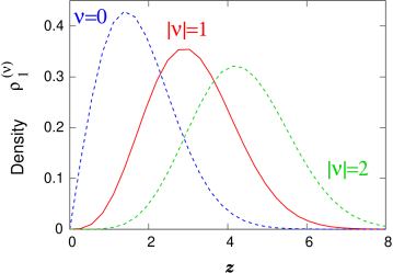
Figure 1: The distributions for the lowest eigenvalue at $|\nu|=0,$ $1$ and $2$, as predicted by chiral RMT.

2.2 Lattice results in the microscopic regime

In order to verify the viability of the $\epsilon$-expansion and of chiral RMT, it is of interest to compare these predictions to the corresponding eigenvalue distributions obtained from lattice simulations. The Wilson Dirac operator seems hardly suitable in this respect; because of the mass renormalization it would be highly problematic to identify the zero modes and the relative values of the remaining modes. In addition, simulations at small quark masses are problematic due to exceptional configurations.

Staggered fermions do not suffer from additive mass renormalization because they have an exact remnant chiral symmetry $\mathop{\rm{}U}\nolimits(1)\otimes\mathop{\rm{}U}\nolimits(1)$. Indeed such comparisons exist. The staggered fermion spectrum agrees well with the RMT prediction in the sector $\nu=0$. However, it turns out that all other sectors, $\nu\neq 0$, yield the same distributions, in particular the same histogram for $\rho^{(\nu)}_{1}(z)$ in QCD [16]. It seems that staggered fermions are generally insensitive to the topology, and therefore not adequate for this purpose, at least for moderate and strong gauge coupling.

Another type of lattice fermions without additive mass renormalization is the Ginsparg-Wilson fermions. Their lattice Dirac operator $D$ fulfills the Ginsparg-Wilson relation (GWR), which reads (in its simplest form)

$$D\gamma_{5}+\gamma_{5}D=\frac{a}{\mu}D\gamma_{5}D\,,$$ (9)

i.e. the continuum condition for the right-hand-side to vanish is relaxed to a term of $O(a)$, where $a$ is the lattice spacing. $\mu$ is a mass parameter, see below. The GWR implies that $D^{-1}\gamma_{5}+\gamma_{5}D^{-1}=a\gamma_{5}/\mu$ is local, therefore the poles in the propagator are not shifted away from zero. Thus the Ginsparg-Wilson fermions have exact zero modes, which occur with positive or negative chirality. We now define the topological charge $\nu$ simply by the index

$$\nu=n_{+}-n_{-}\,,$$ (10)

where $n_{+}$ ($n_{-}$) is the number of positive (negative) chiral zero modes. Here one adapts the continuum Index Theorem and uses it to define the topological charge of the lattice gauge configurations [6, 7]. The applicability of chiral RMT to Ginsparg-Wilson fermions has been discussed theoretically in ref. [21].

Many lattice Dirac operators, such as the Wilson operator $D_{W}$, obey $\gamma_{5}$ Hermiticity, $D_{W}^{\dagger}=\gamma_{5}D_{W}\gamma_{5}$. This allows for a simple solution of the GWR by inserting $D_{W}$ (say with Wilson parameter 1) into the overlap formula [9],

$$D_{\rm ov}=\frac{\mu}{a}\left[1+{A}/{\sqrt{A^{\dagger}A}}\right],\qquad A=aD_{W}-\mu\,.$$ (11)

$D_{\rm ov}$ is a solution to condition (9) and it is $\gamma_{5}$-hermitean as well. (There are alternatives to replace $D_{W}$ by lattice Dirac operators that are more involved but lead to improved properties, as suggested in refs. [22].) $\mu$ represents a negative mass of the Wilson fermion, which can be chosen in some interval as long as the gauge fields are smooth. In the free case $\mu=1$ is optimal with respect to locality, but at $\beta=6$ and $\beta=5.85$ we move to $\mu=1.4$ resp. $\mu=1.6$ to compensate the mass renormalization of the Wilson fermion.

Note that the operator $A/\sqrt{A^{\dagger}A}$ is unitary, hence the spectrum of $D_{\rm ov}$ is located on a circle in the complex plane through zero, with center and radius $\mu/a$. In order to relate the eigenvalues found on this Ginsparg-Wilson circle to the continuum eigenvalues $\lambda_{n}$, we map the circle stereographically onto the imaginary axis. Requiring $f(z)=z+O(z^{2})$ and $f(2\mu)=\infty$ singles out the Möbius transform

$$f(z)=\frac{z}{1-z/(2\mu)}\,.$$ (12)

This mapping has been suggested before in ref. [23], in connection with the Leutwyler-Smilga sum rules [2].

The eigenvalues of Ginsparg-Wilson operators were compared to the RMT prediction for the Schwinger model in ref. [17], where the overlap operator (11) as well as a truncated fixed point Dirac operator were considered. In both cases the results agreed with the RMT formulae.

Such studies were also performed with the overlap operator in 4d QED [18] and again the predictions were successful within the statistical errors.

Finally QCD was considered, but only on small lattices of size $4^{4}$. Ref. [19] used the overlap operator at strong coupling of $\beta=5.1$. Ref. [20] applied a truncated fixed point action and obtained a decent agreement in a volume of $V=(1.2\,{\rm fm})^{4}$. However, when the physical lattice spacing is decreased so that the volume shrinks to $(0.88\,{\rm fm})^{4}$, the leading non-zero eigenvalue distributions of the different topological sectors are on top of each other, in contrast to the RMT prediction.

Our results are obtained by using again the overlap operator (11) in QCD with the standard plaquette gauge action. We have chosen a rather weak gauge coupling, $\beta\geq 5.85$, so that the overlap formula can safely be applied to construct a Ginsparg-Wilson fermion. Due to the computational effort required by the overlap operator we had to use the quenched approximation, as it was also the case in all previous studies mentioned above. We approximated the inverse square root by Chebyshev polynomials to an accuracy of $10^{-12}$. Then we used the PARPACK routines to evaluate up to 100 eigenvalues of $D_{\rm ov}$. We focused on the eigenvalues with the least real parts resp. absolute values. Of course the non-zero eigenvalues occur in complex conjugate pairs, hence we only consider one sign for the imaginary part.

lattice		physical	number of configurations
size	$\beta$	volume	$\nu=0$	$|\nu|=1$	$|\nu|=2$
$12^{4}$	6	$(1.12\,{\rm fm})^{4}$	44	70	24
$10^{4}$	5.85	$(1.23\,{\rm fm})^{4}$	74	112	84
$8^{4}$	5.85	$(0.98\,{\rm fm})^{4}$	80	63	28

Table 1: The statistics of our simulations on three lattice sizes.

First we measured the leading non-zero eigenvalue on a $12^{4}$ lattice at $\beta=6$. Here the volume amounts to $(1.12\,{\rm fm})^{4}$. The result can be represented by a histogram, which could then be compared to figure 1. However, such a picture depends on the (arbitrary) choice of the bin size in the histogram. This can be avoided by plotting the “cumulative density”, see e.g. ref. [25], which sums up all the entries up to the considered value of $z$ — it is normalized so that the full number of entries corresponds to the cumulative density 1. This way to plot the data can be compared to the cumulative density according to the RMT prediction,

$$\rho_{1,c}^{(\nu)}(z)=\frac{\int_{0}^{z}\rho_{1}^{(\nu)}(z^{\prime})dz^{\prime}}{\int_{0}^{\infty}\rho_{1}^{(\nu)}(z^{\prime})dz^{\prime}}\,.$$ (13)

This comparison is done in figure 2 (top). We recognize a satisfactory agreement, especially for $|\nu|=1$, where we have the largest statistics, see table 1. In particular, we do see the effect that the peak of the density — resp. the interval of steepest ascent of the cumulative density — moves to larger values of $z$ for increasing topological charge. In this plot the chiral condensate $\Sigma$ enters as the one free parameter, which sets the energy scale. Our plot is shown for the value

$$\Sigma=(256\,{\rm MeV})^{3}\,,$$ (14)

which provides optimal agreement with the RMT curves.

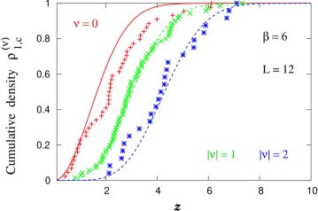
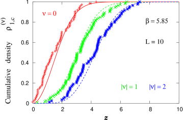
Figure 2: The cumulative distribution of the lowest non-zero eigenvalue at $\beta=6$ on a $12^{4}$ lattice (top), and on a $10^{4}$ lattice at $\beta=5.85$ (bottom). We show the RMT predictions (lines) and result for the indices $|\nu|=0,1,2$. In both cases, in particular at $L=10$, we find a satisfactory agreement with RMT, if the chiral condensate is chosen optimally. This requires $\Sigma=(256{\rm MeV})^{3}$ (top) resp. $\Sigma=(253{\rm MeV})^{3}$ (bottom). The $10^{4}$ lattice corresponds to a somewhat larger physical volume.

Next we studied a $10^{4}$ lattice at $\beta=5.85$, which corresponds to a somewhat larger physical volume of $V=(1.23\,{\rm fm})^{4}$. Again the results for the leading non-zero eigenvalue are shown for the topological sectors $|\nu|=0,1$ and $2$ in figure 2 (bottom). Also here we find a reasonable agreement with the RMT predictions, and the optimal value of the chiral condensate is modified to $\Sigma=(253~{}{\rm MeV})^{3}$. RMT predicts a (logarithmically) increasing $\Sigma(V)$ due to quenching [15]. A conclusive verification of this behavior (beyond possible lattice artifacts) would require further simulations. In figure 3 we show our results for the cumulative density of the next-to-leading eigenvalue at $|\nu|=0$, $1$ and $2$, for both lattices discussed before. Here we do not find a convincing agreement with the RMT prediction in the first ref. of [14]; note that the relevant values of $z$ are larger compared to figure 2. Also the second non-zero eigenvalue moves to larger values of $z$ if $|\nu|$ increases.

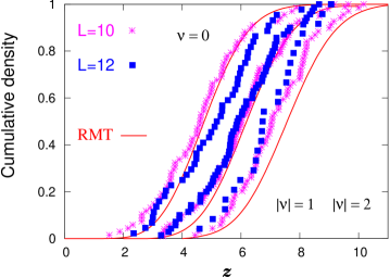
Figure 3: The cumulative density of the second non-zero eigenvalue at $L=12$, $\beta=6$ and at $L=10$, $\beta=5.85$. At $|\nu|=0,$ $1$ and $2$ we do not find a convincing agreement with the RMT prediction (solid lines). Also the second eigenvalue moves to larger values for increasing $|\nu|$.

Now we consider the eigenvalue density without focusing particularly on the first or on the second non-zero eigenvalue (though we still omit the zeros). Then we obtain for instance at $|\nu|=1$ the densities shown in figure 4. RMT predicts an oscillating behavior (see first ref. in [13]), which is also plotted for comparison. We find a good agreement roughly up to the second peak (as expected from figures 2 and 3). Then we are leaving the microscopic regime and turn to the bulk; for the latter the density is supposed to rise as $\lambda^{3}$ resp. $z^{3}$. This is nicely confirmed by our data; an example is illustrated in figure 5.

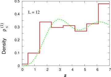
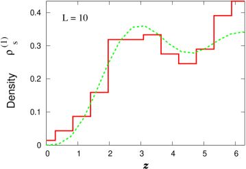
Figure 4: The density of eigenvalues of the Dirac operator in the microscopic regime, for the $12^{4}$ lattice at $\beta=6$ (top) and for the $10^{4}$ lattice at $\beta=5.85$ (bottom). In both cases, we show as an example the data for $|\nu|=1$, which follow the RMT predicted oscillating behavior (dashed line) roughly up to the second peak. If the oscillation is averaged to a plateau, its hight agrees with the eigenvalue density at zero according to the Banks-Casher relation, $\rho(z=0)=\rho(\lambda=0)/\Sigma V=1/\pi$.

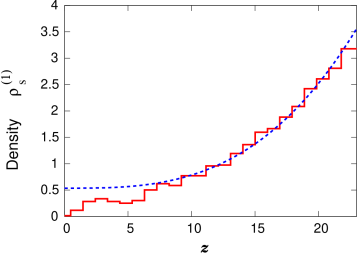
Figure 5: The eigenvalue density on the $12^{4}$ lattice at $\beta=6$, $|\nu|=1$. We see the transition from the microscopic regime to the bulk, where the density follows the predicted increase $c_{0}+c_{1}\lambda^{3}$ (dashed line).

Finally we consider a smaller volume: we use a $8^{4}$ lattice at $\beta=5.85$, which corresponds to $V=(0.98\,{\rm fm})^{4}$. Figure 6 shows that in this case there is a clear disagreement with the RMT prediction; in particular the sensitivity of the peak to $|\nu|$ is lost to a large extent (beyond very small values of $z$). This is in qualitative agreement with the results of ref. [20] on the $4^{4}$ lattice. The observation that the volume has to be $V\gtrsim(1.2\,{\rm fm})^{4}$ can be viewed as an empirical determination of the Thouless energy.

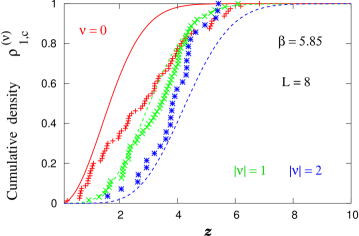
Figure 6: The cumulative density of the lowest non-zero eigenvalue at $\beta=5.85$ on a $8^{4}$ lattice. The data from different topological sectors are close to each other (beyond very small $z$ values), hence in this small volume they do not agree with the RMT curves.

At this point, we would like to add that the above results tend to look similar for the leading eigenvalues of the hermitean overlap Dirac operator

$$H_{\rm ov}=\gamma_{5}D_{\rm ov}\,.$$ (15)

(Of course, in this case the stereographic mapping is not needed.) As an example we show the cumulative density of the first positive (non-zero) eigenvalue of $H_{\rm ov}$ at $L=10$, $\beta=5.85$ in figure 7.

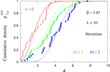
Figure 7: The cumulative density of the lowest non-zero eigenvalue of the hermitean overlap Dirac operator $H_{\rm ov}=\gamma_{5}D_{\rm ov}$ on the $10^{4}$ lattice at $\beta=5.85$.

lattice		confidence level			optimal
size	$\beta$	$\nu=0$	$|\nu|=1$	$|\nu|=2$	$\Sigma$	$\chi_{t}\,r_{0}^{4}$
$12^{4}$	6	0.003	0.73	0.79	$(256~{}{\rm MeV})^{3}$	0.063
$10^{4}$	5.85	0.03	0.48	0.10	$(253~{}{\rm MeV})^{3}$	0.078

Table 2: The results on the two lattices which turned out to be sufficiently large for the data to be compared with the RMT predictions, for the suitable values of $\Sigma$ used in figure 2. We also display the statistical confidence level according to the Kolmogorov-Smirnov test, and our results for the topological susceptibility $\chi_{t}$ ($r_{0}$ is the Sommer parameter).

For completeness we report our statistics in table 1 and summarize the results in table 2. In that table we also include an estimate for the topological susceptibility, where some configurations with higher charges contribute as well. We present the dimensionless quantity $\chi_{t}r_{0}^{4}$, where $\chi_{t}=\langle\nu^{2}\rangle/V$ is the susceptibility and $r_{0}$ is the Sommer parameter obtained from the static quark-antiquark potential [26]. The results are well consistent with the values in the literature (for an overview, see ref. [20, figure 18]), although our statistics is clearly too small for that quantity. (Hence we do not try to estimate errors on $\Sigma$ and $\chi_{t}r_{0}^{4}$.) Finally table 2 also gives the results of the Kolmogorov-Smirnov test [25] for the confidence level of the results obtained, if one assumes the RMT probability distribution to be correct. The corresponding number described the probability for the observed deviation from the theory to occur with the given statistics. This test is just designed for the cumulative density. The results suggest that the volume $(1.12\,{\rm fm})^{4}$ is still somewhat small, so that the topologies are still not fully separated, but we see that this process sets in at least for the first non-zero eigenvalue on volumes larger than that.

2.3 Unfolded distribution

We now turn to another way of comparing our lattice data to a conjecture from RMT. This new evaluation allows us to take all our non-zero eigenvalues into account (for one sign of the imaginary part, i.e. up to 50 for each configuration).

We build from all the eigenvalues of all configurations the “unfolded distribution” as described for instance in ref. [19] (for generalities, see ref. [27]). To this end, we first numerate all available non-zero eigenvalues with positive imaginary part in each configuration in ascending order, given by the angle in the Ginsparg-Wilson circle. Then we put all these eigenvalues from all configurations together and numerate them again in ascending order. Now we consider pairs of eigenvalues from the same configuration, which follow immediately one after the other in the original numeration. If they differ in the global numeration by $k$, then $k/N_{{\rm conf}}$ is the “unfolded level spacing”, where $N_{{\rm conf}}$ is the number of configurations involved.

In figure 8 we show our results for $L=12$, at $\beta=6$ and for $L=8$, at $\beta=5.85$. The histograms are compared to RMT conjectures for different groups and representations, and we can confirm a good agreement with the Wigner distribution predicted for $\mathop{\rm SU}\nolimits(3)$ in the fundamental representation. Considering also ref. [19] we conclude that this property holds over a large range of volumes. Since we include all eigenvalues here, our statistics is much larger than in the plots for the microscopic regime. Note, however, that this analysis is not sensitive to the topology any more.

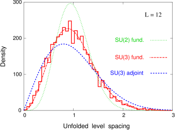
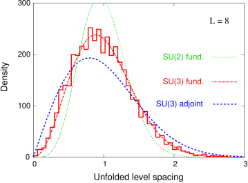
Figure 8: The unfolded level spacing distribution for $\beta=6$ on a $12^{4}$ lattice (top), and for $\beta=5.85$ on a $8^{4}$ lattice (bottom). We find a convincing agreement with the RMT conjecture for the $\mathop{\rm SU}\nolimits(3)$ group in the fundamental representation that we are using. The same also holds for the $10^{4}$ lattice at $\beta=5.85$. (The curves are normalized according to the number of entries in the statistics.)

Moreover the unfolded distribution only tests the correct symmetry group that is to be taken in RMT. There is no physics information such as values for the condensate or the pion decay constant, because one does not keep track of a physical scale. Nevertheless, the unfolded distribution provides a non-trivial test for RMT.

3 Conclusions

We performed a lattice study of quenched QCD using the overlap operator to test RMT predictions for the eigenvalue distributions of the Dirac operator. In this pilot study we worked at $\beta$ values large enough so that the overlap formula can safely be applied as a solution of the GWR. By using lattices of size $8^{4}$, $10^{4}$ and $12^{4}$ we were able to reach physical volumes which are large enough to test RMT.

In the microscopic regime of the very small eigenvalues we observe agreement with the predictions by RMT applied to the $\epsilon$-regime of chiral perturbation theory, if the physical volume is large enough; $V\gtrsim(1.2\,{\rm fm})^{4}$ seems to be sufficient to capture at least the leading non-zero eigenvalue. On smaller physical volumes this agreement — and in particular the sensitivity to the topology — disappears.

If we consider the unfolded level spacing distribution, however, we obtain a good agreement with the RMT conjecture, even down to a small physical volume.

The eigenvalue distributions in figure 2 show interesting characteristic features. In topological charge sector zero the probability for a very low non-zero eigenvalue is non-negligible. Therefore such very low-lying modes will appear in simulations. This might have serious consequences for numerical studies when the quark mass is lowered too much. In particular, this behavior might render simulations in the $\epsilon$-regime problematic. Indications of these difficulties were presented in ref. [4], where also an analysis of the influence of the lowest mode in the $\nu=0$ sector on the measurement of the chiral condensate was given. It was reported that the condensate is very hard to measure in topological charge sector zero, in agreement with the results presented here.

On the other hand, the situation is clearly better in a non-trivial topology. Eigenvalues close to zero are strongly suppressed and a much better signal can be expected.

Note that this phenomenon is not restricted to the quenched approximation considered here but holds also in the full theory. Thus, it can be expected that simulations close to physical values of the pion mass may become extremely expensive. Clearly, contact to chiral perturbation theory is then mandatory to extrapolate to physical pion masses.

3.1 Outlook

We still want to proceed to larger physical volumes. This will hopefully lead to further precision in the agreement for the leading non-zero eigenvalues in the different topological sectors. The larger volume might provide a histogram for the spectral density, which follows the microscopic RMT for several oscillations. With an increased statistics — which may be accessible using the optimized algorithmic techniques described in ref. [28] — we could evaluate the spectral correlators as well. Further values for $\Sigma(V)$ would also allow us to extract an estimation for $F_{\pi}$ [15]. Finally we are also about to extend this analysis to a hypercube overlap fermion, which is described in ref. [29]. This is a different Ginsparg-Wilson fermion, and its study will provide a more complete picture of the spectral behavior of this class of lattice Dirac operators.