Lattice results with three quark flavours

Abstract

There have been exciting advances recently in finite temperature calculations with three quark flavours and with non-zero chemical potential. The role of improved actions is explained and recent results from the Bielefeld group and MILC collaboration with improved Kogut-Susskind quarks are presented. Three new approaches to finite chemical potential are discussed.

1 Introduction

I have been asked by the organizers to review the status of lattice QCD calculations at non-zero temperature with three quark flavours. The exciting news here is that due to improvements in algorithms, we are now able to carry out calculations with light up and down quarks considerably lighter than the strange quark. Before presenting results, I give a brief introduction to lattice calculations, and then I will outline how algorithms have been improved. After presenting numerical results, I will discuss briefly the recent significant advances in dealing with finite chemical potential. (I ran out of time during my talk and did not discuss this at the conference.)

2 Introduction to Lattice Calculations

To carry out a lattice simulation we must select certain parameters, namely the lattice spacing ($a$) or gauge coupling ($\beta$), a fixed grid size ($N_{s}^{3}\times N_{t}$) where $N_{s}$ and $N_{t}$ are the space and time dimensions of the grid, respectively, and quark masses ($m_{u,d}$, $m_{s}$). There are also certain parameters related to the algorithm. The parameters detailed have physical meaning, and each choice can lead to a systematic error that must be controlled.

To deal with the non-zero lattice spacing, we must take the continuum limit. Similarly, we must take the infinite volume limit to deal with the finite fixed grid. Finally, we must extrapolate to light quark mass for the up and down quarks. This is a practical issue as it is too expensive to do the calculations with the physical up and down masses. On the other hand, we can work at the physical $s$ quark mass. For finite temperature calculations, the temperature is given by $T=1/(N_{t}a)$, so we use grids with $N_{t}<N_{s}$. Typically, $N_{s}$ is two or three times $N_{t}$ to provide a reasonably large physical volume.

Also of physical relevance (especially for the RHIC program) is nonzero chemical potential $\mu$. Until recently, it has been nearly impossible to carry out calculations with $\mu\neq 0$.

3 How have algorithms been improved?

The first numerical lattice calculations used the Wilson (plaquette) gauge action and either Wilson or Kogut-Susskind (KS or staggered) quark actions. The Wilson quark action is designed to solve the fermion “doubling” problem. So is the KS approach; however, it maintains enough degrees of freedom for four quark fields. There remains a $U(1)$ chiral symmetry and a single Goldstone pion. The rest of the flavour symmetry is broken for non-zero lattice spacing. Thus, the other pion states are heavier than the Goldstone state because of flavour (or what is now frequently called taste) symmetry breaking.

Starting in the mid-1980s, the Symanzik improvement program [1] began to be applied to calculations to improve the scaling properties of the theory. For Wilson type quarks the improvement called clover quarks was introduced by Sheikholeslami and Wohlert [2]. Naik introduced a new three link term for KS quarks in 1989 [3]. An improved gauge action was applied in 1995 [4]. Soon thereafter calculations were done with the Naik term and an improved gauge action [5] and the importance of “fattening” the action to reduce taste symmetry breaking was tested and understood [6–10]. About the same time, the P4 action was introduced because of it’s improved rotational symmetry [11, 12]

All of these improvement schemes are analagous to higher order methods in numerical analysis, but with the twist of applying to QFT. They exact a computational toll from having a more complicated action, but they more than make up for that by reducing systematic errors and allowing a larger lattice spacing to be used. Since computational requirement goes like a large power (7–9) of the inverse lattice spacing, it really reduces the cost to use a larger lattice spacing.

More recently, domain wall fermions and the overlap method were developed to better control chiral symmetry. They are not yet extensively used for thermodynamics, but see reference [13].

We shall concentrate on the improvement program for staggered quarks. The Bielefeld group is the center of activity for the P4 action that maintains rotational invariance of the free quark propagator to order $p^{4}$,

$$S_{F}(m_{f,L})~{}=~{}c_{1}^{F}S_{1-link,fat}(\omega)+c_{3}^{F}S_{3-link}+m_{f,L}\sum_{x}\bar{\chi}_{x}^{f}\chi_{x}^{f}~{}~{}~{}~{}~{}~{}~{}~{}~{}~{}~{}~{}~{}~{}~{}~{}~{}~{}~{}~{}~{}~{}~{}$$ (1)

$$\equiv \sum_{x}\bar{\chi}_{x}^{f}~{}\sum_{\mu}~{}\eta_{\mu}(x)~{}\Bigg{(}{3\over 8}~{}\Bigg{[}\mbox{ \begin{picture}(2.5,0.2) \put(0.0,0.1){\circle*{0.1}}\put(2.0,0.1){\circle*{0.1}} \put(1.01,0.1){\circle{0.2}} \put(0.8,0.0){\mbox{ \begin{picture}(1.1,0.1)\put(0.0,0.1){\vector(1,0){1.0}} \end{picture}}} \put(-0.2,0.0){\mbox{ \begin{picture}(1.1,0.1)\put(1.0,0.1){\vector(-1,0){1.0}} \end{picture}}} \put(1.1,-0.2){\scriptsize$x$ } \put(0.0,-0.2){\scriptsize$y$ } \put(2.0,-0.2){\scriptsize$y$ } \end{picture}}~{}+~{}\omega~{}~{}\sum_{\nu\neq\mu}~{}~{}\mbox{ \begin{picture}(3.0,0.2) \put(0.0,0.1){\circle*{0.1}}\put(2.4,0.1){\circle*{0.1}} \put(1.21,0.1){\circle{0.2}} \put(1.2,-1.0){\mbox{ \begin{picture}(1.2,2.2)\put(0.0,1.2){\vector(0,1){1.0}} \put(0.0,1.0){\vector(0,-1){1.0}} \put(0.0,2.2){\vector(1,0){1.0}} \put(0.0,0.0){\vector(1,0){1.0}} \put(1.0,0.0){\vector(0,1){1.0}} \put(1.0,2.2){\vector(0,-1){1.0}} \end{picture}}} \put(-0.2,-1.0){\mbox{ \begin{picture}(1.2,2.2)\put(1.0,1.2){\vector(0,1){1.0}} \put(0.0,2.2){\vector(0,-1){1.0}} \put(1.0,2.2){\vector(-1,0){1.0}} \put(1.0,1.0){\vector(0,-1){1.0}} \put(1.0,0.0){\vector(-1,0){1.0}} \put(0.0,0.0){\vector(0,1){1.0}} \end{picture}}} \put(1.1,-0.3){\scriptsize$x$ } \put(-0.4,-0.2){\scriptsize$y$ } \put(2.6,-0.2){\scriptsize$y$ } \end{picture}}\Bigg{]}$$

$$+{1\over 96}~{}\sum_{\nu\neq\mu}~{}\Bigg{[}\mbox{ \begin{picture}(2.5,2.5)\put(0.0,0.0){\circle*{0.1}}\put(0.0,1.0){\circle*{0.1}}\put(0.0,2.0){\circle*{0.1}} \put(1.0,-1.0){\circle*{0.1}}\put(1.0,-2.0){\circle*{0.1}} \put(1.0,0.0){\circle{0.2}} \put(2.0,-2.0){\circle*{0.1}} \put(0.0,1.0){\vector(0,1){1.0}} \put(0.0,0.0){\vector(0,1){1.0}} \put(1.0,0.0){\vector(-1,0){1.0}} \put(1.0,0.0){\vector(0,-1){1.0}} \put(1.0,-1.0){\vector(0,-1){1.0}} \put(1.0,-2.0){\vector(1,0){1.0}} \put(1.25,-0.1){\scriptsize$x$ } \put(2.1,-2.1){\scriptsize$y$ } \put(-0.5,2.0){\scriptsize$y$ } \end{picture}}+\mbox{ \begin{picture}(2.5,2.5)\put(1.0,1.0){\circle*{0.1}}\put(1.0,2.0){\circle*{0.1}} \put(1.0,0.0){\circle{0.2}} \put(2.0,0.0){\circle*{0.1}}\put(2.0,-1.0){\circle*{0.1}}\put(2.0,-2.0){\circle*{0.1}} \put(0.0,2.0){\circle*{0.1}} \put(1.0,2.0){\vector(-1,0){1.0}} \put(1.0,1.0){\vector(0,1){1.0}} \put(1.0,0.0){\vector(0,1){1.0}} \put(1.0,0.0){\vector(1,0){1.0}} \put(2.0,0.0){\vector(0,-1){1.0}} \put(2.0,-1.0){\vector(0,-1){1.0}} \put(0.5,-0.1){\scriptsize$x$ } \put(1.5,-2.1){\scriptsize$y$ } \put(-0.5,2.0){\scriptsize$y$ } \end{picture}}~{}+\mbox{ \begin{picture}(2.5,2.5)\put(1.0,-1.0){\circle*{0.1}}\put(1.0,-2.0){\circle*{0.1}} \put(1.0,0.0){\circle{0.2}} \put(2.0,0.0){\circle*{0.1}}\put(2.0,1.0){\circle*{0.1}}\put(2.0,2.0){\circle*{0.1}} \put(0.0,-2.0){\circle*{0.1}} \put(1.0,-2.0){\vector(-1,0){1.0}} \put(1.0,-1.0){\vector(0,-1){1.0}} \put(1.0,0.0){\vector(0,-1){1.0}} \put(1.0,0.0){\vector(1,0){1.0}} \put(2.0,0.0){\vector(0,1){1.0}} \put(2.0,1.0){\vector(0,1){1.0}} \put(0.5,-0.1){\scriptsize$x$ } \put(1.5,2.0){\scriptsize$y$ } \put(-0.4,-2.1){\scriptsize$y$ } \end{picture}}+\mbox{ \begin{picture}(2.5,2.5)\put(0.0,0.0){\circle*{0.1}}\put(0.0,-1.0){\circle*{0.1}}\put(0.0,-2.0){\circle*{0.1}} \put(1.0,1.0){\circle*{0.1}}\put(1.0,2.0){\circle*{0.1}} \put(1.0,0.0){\circle{0.2}} \put(2.0,2.0){\circle*{0.1}} \put(0.0,-1.0){\vector(0,-1){1.0}} \put(0.0,0.0){\vector(0,-1){1.0}} \put(1.0,0.0){\vector(-1,0){1.0}} \put(1.0,0.0){\vector(0,1){1.0}} \put(1.0,1.0){\vector(0,1){1.0}} \put(1.0,2.0){\vector(1,0){1.0}} \put(1.25,-0.1){\scriptsize$x$ } \put(2.2,2.0){\scriptsize$y$ } \put(-0.4,-2.1){\scriptsize$y$ } \end{picture}}\Bigg{]}\Bigg{)}\chi_{y}^{f}$$

$$+m_{f,L}\sum_{x}~{}\bar{\chi}_{x}^{f}\chi_{x}^{f}\quad.$$

The MILC collaboration uses the “Asqtad” action [8, 9, 10]. Their gauge action includes plaquette, $1\times 2$ and bent 6-link terms. Their quark action includes the links shown below and the 3-link Naik term. The three, five and seven link terms are known as fat links and are necessary to reduce taste symmetry breaking. The full set of fattened links is pictured in figure 1.. The weights of each term are not shown. Each diagram represents a term in the quark action of the form $\bar{\chi}(x)V(x,x+\hat{\mu})\chi(x+\hat{\mu})$, where $V$ is the product of links along the path. With coefficients of the various terms set using tadpole improvement, the errors of this action are of order $a^{2}\alpha$ and $a^{4}$.

Figure 1: Terms used to suppress flavour symmetry breaking. The final five link path was introduced by Lepage to correct the small momentum form factor.

It is easy to see why improved actions should have better high temperature behavior than the Wilson or KS actions. In figure 2, we can examine the energy and pressure for free massless quarks on a lattice with $N_{t}$ time slices [14]. The continuum limit corresponds to $N_{t}\rightarrow\infty$. One immediately sees that both Naik and P4 actions much more rapidly approach the continuum limit than either Wilson or KS quarks. At $N_{t}=4$, Naik is better for pressure and P4 is better for energy density. For $N_{t}=6$, the situation is reversed. For $N_{t}\geq 8$, both improved actions are quite close to the continuum limit, with P4 a little closer.

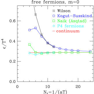
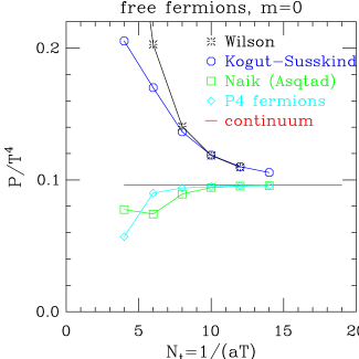
Figure 2: The energy density (left) and pressure (right) of free massless fermions as function of temporal lattice size $N_{t}$.

4 Some recent physics results

We will now concentrate on results with 3 degenerate or 2+1 flavours of quark. Some of the issues to be addressed are: a) what is the phase diagram of QCD?, b) what is the transition temperature?, c) where does the the physical point in the phase diagram lie?, d) what is the equation of state for QCD?

To find the phase diagram, we must find the transition temperature for a variety of quark masses, so it would be logical to address (b) before (a); however, presenting the phase diagram first helps to orient us, so in figure 3, I present a nice summary plot prepared by Karsch of the QCD phase diagram in the $m_{u,d}$-$m_{s}$ plane [15].

Symmetry considerations help us to identify the order of the transition on the corners of the diagram [16]. In the upper right hand corner we have pure gauge theory with a deconfinement transition at $T\approx 270$ MeV. In the lower-left corner of the diagram, we expect a first order transition for three massless degenerate flavours. Chiral symmetry is broken at low temperature and restored at high temperature. We expect that as the quark masses are increased, the transition will weaken as we approach a second order line. When the strange quark is very heavy, but $u$ and $d$ are light, we expect a second order transition for massless quarks. Karsch’s estimates of the chiral transition temperatures in the corners are shown in the diagram.

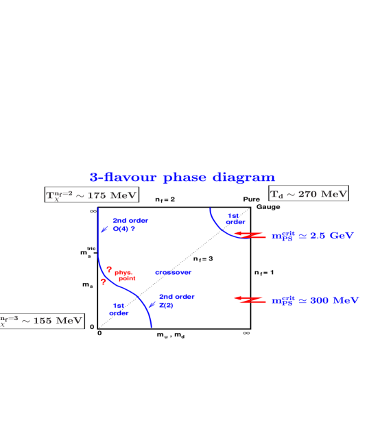
Figure 3: From F. Karsch [15].

Some recent results from the MILC collaboration [17] with the Aqstad action and either 2+1 or 3 degenerate flavours indicate that above 175–200 MeV $\langle\bar{\psi}\psi\rangle$ extrapolates to 0 as $m_{q}\rightarrow 0$. This is evidence that chiral symmetry is restored at higher temperature. For 2+1 flavours, with $N_{t}=6$, the chiral symmetry restoration starts at about 200 MeV. The runs with $N_{t}=8$ continue as the lightest quark mass runs are not completed. Here it appears the transition may occur at about 175 MeV. The difference can be a finite lattice spacing effect. Calculations have also been done with three degenerate quarks. The lightest quark mass explored by MILC is 0.4 $m_{s}$ where $m_{s}$ is the strange quark mass. Each of the individual curves looks quite smooth, so it is not clear that any of these masses are within the first order transition region; however, if the curves are extrapolated to zero quark mass, there appears to be chiral symmetry restoration around 185 MeV.

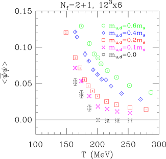
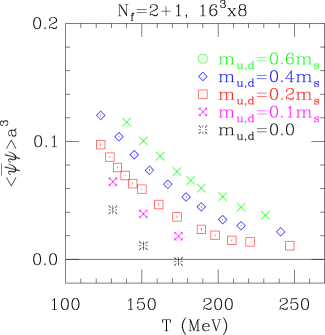
Figure 4: $\langle\bar{\psi}\psi\rangle$ vs. temperature for various light quark masses. Bursts are extrapolations to zero quark mass. These graphs are updated from the ones in reference [17].

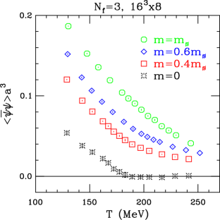
Figure 5: $\langle\bar{\psi}\psi\rangle$ for three degenerate quarks with $N_{t}=8$.

Turning now to the P4 action, Karsch, Laermann and Peikert have done an extensive study with $N_{t}=4$ [18]. A graph summarizing their results for the ratio of $T_{c}$ to the vector meson mass is show in figure 6. For $N_{f}=2$ they show both the P4 action and the standard KS action results. Clearly, the improved action gives a higher value for $T_{c}$. With three degenerate flavours, the transition temperature is lower than for $N_{f}=2$ (considering only improved action results). One combination of quark masses is available for $N_{f}=2+1$; however, the result looks very much like the $N_{f}=2$ result. This could be because the strange quark mass is so much larger than its physical value. The Bielefelders estimate that in the chiral limit $T_{c}=173\pm 8$ MeV for $N_{f}=2$ and $154\pm 8$ MeV for $N_{f}=3$.

We see that the two groups do not seem to be in close agreement on the transition temperature for $N_{f}=3$. A careful comparison would be useful. It is possible that the difference is a finite lattice spacing effect.

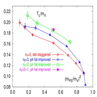
Figure 6: Ratio of transition temperature to vector ($rho$) mass vs. squared ratio of pseudoscalar to vector masses [18]. Results are shown for various numbers of dynamical quarks. For $N_{f}=2$ results with an unimproved action are shown for comparison.

We would like to find the line in the phase diagram separating the first order transition region for very light quarks from the crossover region for heavier quarks.

MILC is exploring a horizontal line at fixed $m_{s}$ and the diagonal with $m_{s}=m_{ud}$. The results shown for $\langle\bar{\psi}\psi\rangle$ are rather smooth curves except perhaps for the lightest quark mass studied on the $16^{3}\times 8$ lattice. MILC does not claim to have worked at light enough quark mass to be in the first order transition region. Two other groups have also studied this question. Karsch, Laermann & Schmidt [19] and Christ & Liao [20] have used light quarks with $N_{t}=4$ and the unimproved action. Both groups are now using the Binder cumulant method to determine the order of the transition. In figure 7, the Binder cumulant is shown as a function of quark mass for three different spatial volumes. The lines should cross at the critical point, which appears to be about 0.035 in lattice units.

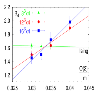
Figure 7: Binder cumulant from Karsch, Laermann & Schmidt [19]. Results from different volumes should cross at the critical point separating the first order region from the smooth crossover.

The two groups estimate the pseudoscalar mass at the critical point to be 270 and 290 MeV. Karsch et al. have some results with the P4 action for which $M_{ps}\approx 192(25)$ MeV. Clearly, given the difference between the unimproved and P4 actions, more work to control the cutoff effects is needed to capitalize on these exploratory works. Also, as interesting as is the three degenerate flavour case, we are most interested in $m_{s}>m_{ud}$.

The pressure of the quark-gluon plasma is of great interest. Using the P4 action, Karsch, Laermann and Peikert [21] have done an extensive study for $N_{t}=4$. Good control of flavour symmetry is important near $T_{c}$ because there is a system of light hadrons, and flavour symmetry breaking distorts the spectrum of the light hadrons. Some fattening is used in this calculation to improve flavour symmetry, but it would be necessary to repeat the calculation with large $N_{t}$, i.e., smaller lattice spacing to get reliable results near $T_{c}$. However, far above $T_{c}$, these results may be indicative of the continuum limit. Figure 8 shows the pressure using the P4 action for various combinations of quark mass and flavours. Indicated by arrows are the free quark values at very high temperature. In the second graph, each pressure curve is normalized by the corresponding value. A comparison with unimproved action results and an estimate of the continuum limit at high temperature is in figure 9.

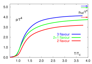
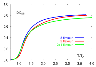
Figure 8: Pressure for various numbers of flavours [21]. For $N_{s}=2$ and 3, $m_{q}=0.4T$. For 2+1, $m_{u,d}=0.4T$ and $m_{s}=T$.

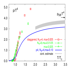
Figure 9: Pressure estimate by Karsch, Laermann and Peikert [21] of continuum limit for $T>2T_{c}$.

5 Strange Quark Content of QGP

MILC has looked at various quark number susceptibilites [17]. They have been related to event-by-event fluctuations in heavy ion collisions in work by B. Muller [22] using the fluctuation-dissipation theorem.

$$\left\langle\delta Q^{2}\right\rangle\propto\frac{T}{V_{s}}\frac{\partial^{2}\log Z}{\partial\mu^{2}_{Q}}=\chi_{Q}(T,\mu_{Q}=0)~{},$$ (2)

We define:

$$\chi_{ij}=\frac{T}{V_{s}}\frac{\partial^{2}\log Z}{\partial\mu_{i}\partial\mu_{j}}\Bigg{|}_{\mu=0}~{},$$ (3)

$$\chi_{sing}=2\chi_{uu}+2\chi_{ud}$$ (4)

and triplet quark number susceptibility

$$\chi_{trip}=2\chi_{uu}-2\chi_{ud}~{}.$$ (5)

As seen in the second part of figure 10, the difference between $\chi_{sing}$ and $\chi_{trip}$ is most pronounced around the transition temperature. MILC also has results for the strange quark susceptibility. It would be useful to try to turn these results into a statement about the strangeness content of the QGP in a way that is testable at RHIC.

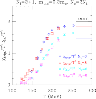
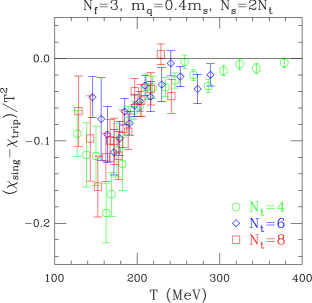
Figure 10: Left: The triplet and strange quark number susceptibilities for $N_{f}=2+1$ with $m_{u,d}=0.2\,m_{s}$ on $12^{3}\times 6$ and $16^{3}\times 8$ lattices [17]. Right: The difference between singlet and triplet quark number susceptibility for $N_{f}=3$ with quarks of mass $m_{q}=0.4\,m_{s}$, on $8^{3}\times 4$, $12^{3}\times 6$ and $16^{3}\times 8$ lattices.

6 Nonzero Chemical Potential

Due to lack of time, this material was not presented in my talk. That was unfortunate, because very significant progress has been made in algorithms, and we can expect to see concomitant advances in calculations soon.

Calculations with finite chemical potential are important because experiments at heavy-ion colliders such a RHIC start with nuclei, not anti-nuclei so there is a quark chemical potential $\mu$ of about 15 MeV [23]. However, finite chemical potential is difficult because the action is no longer real so it is no longer possible to implement importance sampling in the usual way. Recent progress has been made using three new methods.

Fodor and Katz introduced a multiparameter reweighting technique [24]. The key here is that the gauge coupling is shifted from $\beta$ to $\beta_{0}$ in order to maximize the overlap of the ensemble generated with $\mu=0$ with the desired $\mu\neq 0$ ensemble. This is detailed in (6) and illustrated in figure 11 [25].

$$Z(\beta,\mu,m)=\int{\cal D}U\exp[-S_{g}(\beta)]\det M(\mu,m)$$

$$=\int{{\cal D}U\exp[-S_{g}(\beta_{0})]\det M(\mu=0,m)}$$ (6)

$${\times\left\{\exp[-S_{g}(\beta)+S_{g}(\beta_{0})]\frac{\det M(\mu,m)}{\det M(\mu=0,m)}\right\}},$$

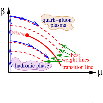
Figure 11: Best weight lines in $\mu-\beta$ plane [25].

A second method introduced by a Swansea-Bielefeld group uses a Taylor series expansion in $\mu/T$ of both the reweighting factor and observable variables [26]. Thus, reweighting is avoided but the chemical potential must be small as only the leading order term is available.

de Forcrand and Philipsen use analytic continuation from imaginary $\mu$ [28, 27]. When the chemical potential is imaginary, the action is real and importance sampling works. The challenge is to do the analytic continuation. It will be interesting to see which of these approaches is best. We are certainly learning more about QCD with $\mu\neq 0$ than we had previously been able to.

7 Prospects

I hope I have convinced you that there are many interesting calculations being done at finite temperature with $N_{f}=2+1$ and 3. However, a great deal remains to be done: we need better control of systematic errors, including the continuum limit and wider coverage of the phase diagram. I have concentrated on results with improved KS type quarks, but these are not the only methods for quarks. For example, improved actions for Clover quarks are being pursued by the CP-PACS/JLQCD collaborations [29]. Dynamical quark calculations with domain wall or overlap quarks and calculations with chemical potential are just in their infancy. Although we lattice practitioners have learned a great deal recently, there is much we can and shall do to improve our calculations.

References

References

- [1] K. Symanzik, Nucl. Phys. B 226, 187 (1983).
- [2] B. Sheikholeslami and R. Wohlert, Nucl. Phys. B 259, 572 (1985).
- [3] S. Naik, Nucl. Phys. B 316, 239 (1989).
- [4] M. G. Alford, W. Dimm, G. P. Lepage, G. Hockney and P. B. Mackenzie, Phys. Lett. B 361, 87 (1995); [arXiv:hep-lat/9507010]. G. P. Lepage, Nucl. Phys. Proc. Suppl. 47, 3 (1996). [arXiv:hep-lat/9510049].
- [5] C. W. Bernard et al. [MILC Collaboration], Nucl. Phys. Proc. Suppl. 53, 212 (1997); [arXiv:hep-lat/9608102]. Phys. Rev. D 58, 014503 (1998); [arXiv:hep-lat/9712010]. Nucl. Phys. Proc. Suppl. 63, 182 (1998). [arXiv:hep-lat/9711013].
- [6] T. Blum et al., Phys. Rev. D 55, 1133 (1997) [arXiv:hep-lat/9609036].
- [7] J. F. Lagae and D. K. Sinclair, Phys. Rev. D 59, 014511 (1999) [arXiv:hep-lat/9806014].
- [8] G. P. Lepage, Phys. Rev. D 59, 074502 (1999) [arXiv:hep-lat/9809157].
- [9] K. Orginos, D. Toussaint and R. L. Sugar [MILC Collaboration], Phys. Rev. D 60, 054503 (1999) [arXiv:hep-lat/9903032].
- [10] C. W. Bernard et al. [MILC Collaboration], Phys. Rev. D 61, 111502 (2000) [arXiv:hep-lat/9912018].
- [11] J. Engels, R. Joswig, F. Karsch, E. Laermann, M. Lutgemeier and B. Petersson, Phys. Lett. B 396, 210 (1997) [arXiv:hep-lat/9612018].
- [12] U. M. Heller, F. Karsch and B. Sturm, Phys. Rev. D 60, 114502 (1999) [arXiv:hep-lat/9901010].
- [13] P. Chen et al., Phys. Rev. D 64, 014503 (2001) [arXiv:hep-lat/0006010].
- [14] C. Bernard et al., Nucl. Phys. A 702, 140 (2002) [arXiv:hep-lat/0110030].
- [15] F. Karsch, Nucl. Phys. A 698, 199 (2002) [arXiv:hep-ph/0103314].
- [16] R. D. Pisarski and F. Wilczek, Phys. Rev. D 29, 338 (1984).
- [17] C. Bernard et al. [MILC Collaboration], Nucl. Phys. Proc. Suppl. 119, 523 (2003) arXiv:hep-lat/0209079.
- [18] F. Karsch, E. Laermann and A. Peikert, Nucl. Phys. B 605, 579 (2001) [arXiv:hep-lat/0012023].
- [19] F. Karsch, E. Laermann and C. Schmidt, Phys. Lett. B 520, 41 (2001) [arXiv:hep-lat/0107020].
- [20] N.H. Christ and X. Liao, Nucl. Phys. Proc. Suppl. 119, 514 (2003).
- [21] F. Karsch, E. Laermann and A. Peikert, Phys. Lett. B 478, 447 (2000) [arXiv:hep-lat/0002003].
- [22] B. Muller, Nucl. Phys. A 702, 281 (2002) [arXiv:nucl-th/0111008].
- [23] P. Braun-Munzinger, D. Magestro, K. Redlich and J. Stachel, Phys. Lett. B 518, 41 (2001) [arXiv:hep-ph/0105229].
- [24] Z. Fodor and S. D. Katz, Phys. Lett. B 534, 87 (2002) [arXiv:hep-lat/0104001].
- [25] F. Csikor, G. I. Egri, Z. Fodor, S. D. Katz, K. K. Szabo and A. I. Toth, arXiv:hep-lat/0209114.
- [26] C. R. Allton et al., Phys. Rev. D 66, 074507 (2002) [arXiv:hep-lat/0204010].
- [27] P. de Forcrand and O. Philipsen, arXiv:hep-lat/0209084.
- [28] P. de Forcrand and O. Philipsen, Nucl. Phys. B 642, 290 (2002) [arXiv:hep-lat/0205016].
- [29] S. Aoki et al. [CP-PACS Collaboration], arXiv:hep-lat/0211034.