Lattice Gauge Fixing and the Violation of Spectral Positivity

Abstract

Spectral positivity is known to be violated by some forms of lattice gauge fixing. The most notable example is lattice Landau gauge, where the effective gluon mass is observed to rise rather than fall with increasing distance. We trace this violation to the use of quenched auxiliary fields in the lattice gauge fixing process, and show that violation of spectral positivity is a general feature of quenching. We illustrate this with a simple quenched mass-mixing model in continuum field theory, and with a quenched form of the Ising model. For lattice gauge fixing associated with Abelian projection and lattice Landau gauge, we show that spectral positivity is violated by processes similar to those found in quenched QCD. For covariant gauges parametrized by a gauge-fixing parameter $\alpha$, the $SU(2)$ gluon propagator is well described by a simple quenched mass-mixing formula. The gluon mass parameter appears to be independent of $\alpha$ for sufficiently large $\alpha$.

Although many observables can be determined in lattice gauge theories without gauge fixing, there are several reasons why gauge fixing is desirable in lattice simulations. Gauge fixing is necessary to make the connection between continuum and lattice gauge fields. Continuum theories of the origin of confinement often make predictions about the gauge field propagator. Gauge fixing has also been a key technique in lattice studies of confinement as well.Greensite:2003bk Important properties of the quark-gluon plasma phase of QCD, such as screening masses, are contained in the finite-temperature gluon propagator.

Techniques for lattice gauge fixing have been known for some time.Mandula It has been clear from the beginning that non-Abelian lattice gauge field propagators show a violation of spectral positivity. This is readily seen from the effective mass: for a normal operator which connects only states of positive norm to the vacuum, the effective mass monotonically decreases with distance to the lightest mass state coupling to the operator. Covariant gauge gluon propagators have an effective mass increasing with distance. In one sense, this is not surprising. We know from perturbation theory that covariant gauges contain states of negative norm. However, that knowledge has neither explained the form of the lattice gluon propagator nor aided in the interpretation of the mass parameters measured from it. In fact, no similar violation of spectral positivity is observed in the $U(1)$ case Coddington:yz , which has negative-norm states in covariant gauges.

In lattice simulations, gauge fixing has typically involved choosing a particular configuration on each gauge orbit. A brief review of this approach is given in Ref. Mandula:nj . In the continuum, on the other hand, gauge fixing usually includes a parameter that causes the functional integral to peak around a particular configuration on the gauge orbit. As shown below, the extension of this idea to lattice gauge theories makes clear that lattice gauge fixing is a form of quenching, with the gauge transformations acting as quenched fields. As has been demonstrated in quenched QCD, quenching can violate spectral positivity, with significant effects on many observables.Golterman:1994jr ; Bardeen:2001yz

We begin with a review of lattice gauge fixing, including the generalization of lattice Landau gauge to covariant gauges with a gauge parameter.Zwanziger:tn ; Parrinello:1990pm ; Fachin:1991pu This generalization will be directly interpreted as a quenched Higgs theory. We then explore the origin of violations of spectral positivity in some simple lattice and continuum models of quenching. Simulation results for the effective mass of an $SU(2)$ lattice gauge field will show behavior very similar to these models as the gauge fixing parameter is varied. We will argue that spectral positivity violations in both lattice covariant gauges and in studies of Abelian projection originate in the quenching process.

The standard approach to lattice gauge fixing is a two step process.Mandula:nj An ensemble of lattice gauge field configurations is generated using standard Monte Carlo methods, corresponding to a functional integral

$$Z_{U}=\int\left[dU\right]e^{S_{U}\left[U\right]}\ ,$$ (1)

where $S_{U}$ is a gauge-invariant action for the gauge fields, e.g., the Wilson action. The gauge action $S_{U}$ is invariant under gauge transformations of the form $U_{\mu}\left(x\right)\rightarrow g\left(x\right)U_{\mu}\left(x\right)g^{+}\left(x+\mu\right)$.

In order to measure gauge-variant observables, each field configuration in the $U$-ensemble may be placed in a particular gauge, i.e., a gauge transformation is applied to each configuration in the $U$-ensemble which moves the configuration along the gauge orbit to a gauge-equivalent configuration satisfying a lattice gauge fixing condition. The simplest gauge choice is defined by maximizing $\sum_{x,\mu}Tr\,\left[U_{\mu}\left(x\right)+U_{\mu}^{+}\left(x\right)\right]$ for each configuration over the class of all gauge transformations. Any local extremum of this functional satisfies a lattice form of the Landau gauge condition:

$$\sum_{\mu}\left[A_{\mu}\left(x+\mu\right)-A_{\mu}\left(x\right)\right]=0$$ (2)

where $A_{\mu}\left(x\right)$ is a lattice approximation to the continuum gauge field, given by

$$A_{\mu}\left(x\right)=\frac{U_{\mu}\left(x\right)-U_{\mu}^{+}\left(x\right)}{2i}-\frac{1}{N}Tr\left[\frac{U_{\mu}\left(x\right)-U_{\mu}^{+}\left(x\right)}{2i}\right]\text{.}$$ (3)

Other gauge-fixing conditions may also be used Giusti:2001xf , and lattice improvement techniques can be applied to the definition of $A_{\mu}$ to reduce discretization errors as well. The global maximization needed is often implemented as a local iterative maximization. The issue of Gribov copies arises in lattice gauge fixing because such a local algorithm tends to find local maxima of the gauge-fixing functional. There are variations on the basic algorithm that ensure a unique choice from among local maxima.Giusti:2001xf

For analytical purposes, it is necessary to generalize this procedure Fachin:1991pu , so that a given single configuration of gauge fields will be associated with an ensemble of configurations of $g$-fields. We will generate this ensemble using

$$S_{gf}\left[U,g\right]=\sum_{l}\frac{\alpha}{2N}Tr\,\left[g\left(x\right)U_{\mu}\left(x\right)g^{+}\left(x+\mu\right)+g\left(x+\mu\right)U_{\mu}^{+}\left(x\right)g^{+}\left(x\right)\right]$$ (4)

as a weight function to select an ensemble of $g$-fields. The sum over $l$ is a sum over all links of the lattice. The normal gauge-fixing procedure is formally regained in the limit $\alpha\rightarrow\infty$. Computationally, this can be implemented as a Monte Carlo simulation inside a Monte Carlo simulation.

Note that the $g$-fields must be thought of as quenched variables, since they do not affect the $U$-ensemble. The expectation value of an observable $O$, gauge-invariant or not, is given by

$$\left\langle O\right\rangle=\frac{1}{Z_{U}}\int\left[dU\right]\,e^{S_{U}\left[U\right]}\frac{1}{Z_{gf}[U]}\int\left[dg\right]e^{S_{gf}\left[U,g\right]}\,O\ ,$$ (5)

where

$$Z_{gf}[U]=\int\left[dg\right]e^{S_{gf}\left[U,g\right]}\text{.}$$ (6)

Formally, the field $g$ is a quenched scalar field with two independent symmetry groups, $G_{global}\otimes G_{local}$, so that it appears to be in the adjoint representation of the gauge group, but the left and right symmetries are distinct. The generating functional $Z_{gf}[U]$ is in some ways a lattice analog of the inverse of the Fadeev-Popov determinant.Bock:2000cd However, there are important differences. Note immediately that $Z_{gf}[U]$ depends on the gauge-fixing parameter $\alpha$. More fundamentally, the lattice formalism resolves the Gribov ambiguity. By construction, gauge-invariant observables are evaluated by integrating over all configurations. Gauge-variant quantities receive contributions from Gribov copies, always with positive weight. Thus the connection between this formalism for lattice gauge fixing and gauge fixing in the continuum is not simple. Furthermore, alternative lattice gauge fixing procedures have been proposed, along with new gauge choices specific to the lattice. A comprehensive review of gauge fixing technology is available.Giusti:2001xf

We begin our analysis of spectral positivity violation with the simplest model of quenching possible: two free, real scalar fields with a non-diagonal mass matrix. The Lagrangrian is

$$L=\frac{1}{2}\left[\left(\partial\phi_{1}\right)^{2}+m_{1}^{2}\phi_{1}^{2}\right]+\frac{1}{2}\left[\left(\partial\phi_{2}\right)^{2}+m_{2}^{2}\phi_{2}^{2}\right]-\mu^{2}\phi_{1}\phi_{2}\ .$$ (7)

We treat the quenched approximation of this model in a manner completely parallel to our discussion of lattice gauge fixing above. We divide the action into three parts $S=S_{1}+S_{2}+S_{12}$, where $S_{1}$ and $S_{2}$ are functionals only of $\phi_{1}$ and $\phi_{2}$, respectively, and $S_{12}$ contains the mixing term. We quench the field $\phi_{2}$. Although there are no loops in this simple theory, quenching implies that $\phi_{2}$ cannot appear as an internal line in the complete propagators. The generating functional in the quenched approximation, including sources $J_{1}$ and $J_{2}$ is

$$Z=\int\left[d\phi_{1}\right]e^{-S_{1}+\int J_{1}\phi_{1}}\frac{\int\left[d\phi_{2}\right]e^{-S_{2}-S_{12}+\int J_{2}\phi_{2}}}{\int\left[d\widetilde{\phi}_{2}\right]e^{-S_{2}-S_{12}}}\text{.}$$ (8)

where we have introduced a kind of ghost variable $\widetilde{\phi}_{2}$; space-time variables are implicit.

Figure 1: Exact propagator for the quenched $\phi_{2}$ field in the simple mass mixing model.

From the generating functional we can obtain the $\left\langle\phi_{1}\phi_{1}\right\rangle$ and $\left\langle\phi_{2}\phi_{2}\right\rangle$ propagators. In momentum space, the $\left\langle\phi_{1}\phi_{1}\right\rangle\,$propagator is $1/(p^{2}+m_{1}^{2})$, since $\phi_{1}$ is unaffected by $\phi_{2}$. On the other hand, the $\left\langle\phi_{2}\phi_{2}\right\rangle$ propagator is

$$\frac{1}{p^{2}+m_{2}^{2}}+\frac{1}{p^{2}+m_{2}^{2}}\mu^{2}\frac{1}{p^{2}+m_{1}^{2}}\mu^{2}\frac{1}{p^{2}+m_{2}^{2}}\text{.}$$ (9)

An alternative diagrammatic procedure is to sum Dyson’s series, as shown in Fig. 1, noting that the $\left\langle\phi_{2}\phi_{2}\right\rangle$ propagator is truncated at two terms. The propagator has a structure similar to the $\eta^{\prime}$ propagator in quenched QCD Golterman:1994jr ; Bardeen:2001yz ; the $\eta^{\prime}$ has a double pole form in quenched QCD when singlet self-energy graphs are approximated by a constant. The $\left\langle\phi_{2}\phi_{2}\right\rangle$ propagator also may be written as

$$\left(1-\frac{\mu^{4}}{\left(m_{2}^{2}-m_{1}^{2}\right)^{2}}\right)\allowbreak\frac{1}{p^{2}+m_{2}^{2}}+\frac{\mu^{4}}{\left(m_{2}^{2}-m_{1}^{2}\right)^{2}}\frac{1}{p^{2}+m_{1}^{2}}+\frac{\mu^{4}}{m_{1}^{2}-m_{2}^{2}}\allowbreak\frac{1}{\left(p^{2}+m_{2}^{2}\right)^{2}}\text{.}$$ (10)

This propagator always violates spectral positivity because of the double pole term, $1/\left(p^{2}+m_{2}^{2}\right)^{2}$, which has a coefficient whose sign depends on $m_{1}^{2}-m_{2}^{2}$. Another possible violation of spectral positivity occurs for sufficiently strong mixing: if $\mu^{4}>\left(m_{2}^{2}-m_{1}^{2}\right)^{2}$, there is a simple pole at $p^{2}=-m_{2}^{2}$ with negative residue.

The form of the $\left\langle\phi_{2}\phi_{2}\right\rangle$ propagator in coordinate space is very interesting, and forms the basis for our study of other quenched theories. In any number of dimensions, we can consider propagators using wall sources, i.e., of co-dimension $1$. This has the effect of setting the momentum equal to zero in all the directions of the wall. For wall sources, we have the propagator

$$G(x) = \left(1-\frac{\mu^{4}}{\left(m_{2}^{2}-m_{1}^{2}\right)^{2}}\right)\allowbreak\frac{1}{2m_{2}}e^{-m_{2}\left|x\right|}+\frac{\mu^{4}}{\left(m_{2}^{2}-m_{1}^{2}\right)^{2}}\frac{1}{2m_{1}}e^{-m_{1}\left|x\right|}$$ (11)

$$+\frac{\mu^{4}}{m_{1}^{2}-m_{2}^{2}}\frac{1}{4m_{2}^{3}}e^{-m_{2}\left|x\right|}\left(1+m_{2}\left|x\right|\right)\allowbreak\text{.}$$

The factor $m_{2}\left|x\right|e^{-m_{2}\left|x\right|}$ shows an initial rise rather than a decay with increasing $\left|x\right|$, violating spectral positivity.

We define an effective mass associated with the $\phi_{2}$ field as

$$m_{eff}(x)=\lim_{a\rightarrow 0}\frac{1}{a}\ln\left(\frac{G(x)}{G(x+a)}\right)=-\frac{d}{dx}\ln(G(x))\text{.}$$ (12)

One can easily check explicitly that $m_{eff}(x)\rightarrow\min(m_{1},m_{2})\,$ as $x\rightarrow\infty$. For any field theory which obeys spectral positivity, $m_{eff}(x)$ monotonically decreases to its limiting value. Theories violating spectral positivity may display a complicated behavior for $m_{eff}(x)$ before the eventual onset of asymptotic behavior.

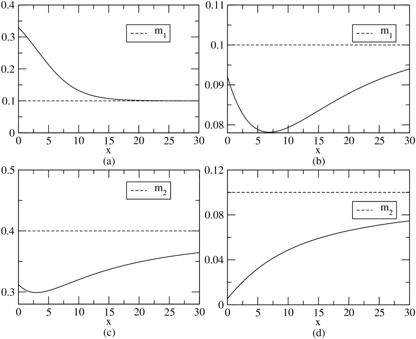
Figure 2: The effective mass associated with $\phi_{2}$ as a function of $x$. The parameters used are: (a) $m_{1}=0.1$, $m_{2}=0.4$, $\mu=0.2$; (b) $m_{1}=0.1$, $m_{2}=0.2$, $\mu=0.2$; (c) $m_{1}=0.5$, $m_{2}=0.4$, $\mu=0.4$; (d) $m_{1}=0.5$, $m_{2}=0.1$, $\mu=0.4$.

We have identified three different possible behaviors for $m_{eff}(x)$ in this simple quenched model. If the mixing parameter $\mu$ is sufficiently small and $m_{1}<m_{2}$, $m_{eff}(x)$ monotonically decreases to its value at infinity, as in a normal field theory which obeys spectral positivity, as shown in Fig. 2(a). As $\mu$ is increased relative to $m_{1}$ and $m_{2}$, $m_{eff}(x)$ may develop a minimum, as displayed in Fig. 2(b). On the other hand, if $m_{2}<m_{1}$, the behavior seen in Fig. 2(a) is not possible, and only the behaviors seen in Fig. 2(c) and Fig. 2(d) are possible. In Fig. 2(d), the minimum has moved to $x=0$. For sufficiently small $\mu$, these effects are difficult to observe, and $m_{eff}(x)$ is essentially equal to $m_{2}$ for all $x$. Regardless of the relative size of $m_{1}$ and $m_{2}$, an observable violation of spectral positivity associated with $m_{eff}(x)$ not monotonically decreasing indicates a significant mixing parameter $\mu$.

Similar behavior can be observed in a very simple lattice model based on the Ising model, where real-space arguments can be used to find an approximate propagator. We consider two coupled one-dimensional Ising models, with spins $\mu_{i}$, $\sigma_{i}\in\left\{-1,+1\right\}$ and respective nearest-neighbor couplings $J$ and $K$. The $\sigma$ spins are coupled to the $\mu$ spins via an interaction of the form $\sum_{i}L\sigma_{i}\mu_{i}$, and the $\sigma$’s are quenched. This simple model is a form of spin glass, with the averaging over the ensemble of $\mu$ spins representing the “quenching” process.

The $\sigma\,$propagator is given by

$$\left\langle\sigma_{0}\sigma_{n}\right\rangle=\frac{1}{Z_{\mu}}\sum_{\left\{\mu\right\}}\exp\left[\sum_{i}J\mu_{i}\mu_{i+1}\right]\frac{1}{Z_{\sigma}\left[\mu\right]}\sum_{\left\{\sigma\right\}}\sigma_{0}\sigma_{n}\exp\left[\sum_{i}\left(K\sigma_{i}\sigma_{i+1}+L\sigma_{i}\mu_{i}\right)\right]\ ,$$ (13)

where $Z_{\mu}$ is the partition function for $\mu$ and $Z_{\sigma}[\mu]$ is the partition function for $\sigma$ in the presence of a particular $\mu$ background. The parameter $L\,$is a mixing parameter. We can approximately evaluate the $\sigma\,$propagator for $J$, $K$, and $L$ sufficiently small by considering the direct contribution $\left(\tanh K\right)^{n}$ combined with mixing of $\sigma\,$with $\mu$. This indirect term can be written as (compare Fig. 1)

$$\sum_{p=1}^{n}\sum_{m=0}^{n-p}\left(\tanh K\right)^{n-p}\left(\tanh L\right)^{2}\left(\tanh J\right)^{p}.$$ (14)

After performing the summations, the propagator is given approximately as

$$\left\langle\sigma_{0}\sigma_{n}\right\rangle\approx\left(\tanh K\right)^{n}+\left(\tanh L\right)^{2}\left(\tanh K\right)^{n}\left[\frac{nx}{\left(1-x\right)}-\frac{x^{2}(1-x^{n})}{\left(1-x\right)^{2}}\right]\ .$$ (15)

where $x=\allowbreak$ $\tanh J/\tanh K$. The $n(\tanh K)^{n}$ factor signals a violation of spectral positivity, just as the $m\left|x\right|\exp\left(-m\left|x\right|\right)$ term did in the mixing model. Of course, the arguments which led to Eq. (9) and Eq. (15) are essentially the same, but carried out in momentum space and real space, respectively. For small $J$, $K$, and $L$, Eq. (15) fits lattice simulations of the $\left\langle\sigma_{0}\sigma_{n}\right\rangle$ propagator well.

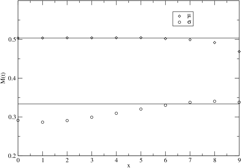
Figure 3: Effective masses for $\sigma$ and $\mu$ in the $1-d$ Ising model.

In Fig. 3, we show the effective mass determined from the $\left\langle\sigma_{0}\sigma_{n}\right\rangle$ and $\left\langle\mu_{0}\mu_{n}\right\rangle$ propagators for the parameter set $J=0.7$, $K=0.9$, and $L=0.3$ for a one-dimensional lattice of size $26$. The propagators were obtained from $40000$ heat bath sweeps of the $\mu$ variables; after each such sweep, $100$ heat bath sweeps of the $\sigma$ variables were carried out. The parameters $K$ and $L$ were chosen empirically so as to display a clear violation of spectral positivity. The $\mu$ mass fits very well with the analytical solution $m=-\ln\tanh(J)$ for the $d=1$ Ising model out to a distance of $8$. Note that the $\sigma$ reaches its asymptotic value of $-\ln(\tanh K)$ from below, and only at $n\simeq 8$. The similarity to the simple field theoretic model of quenching is clear.

We will now show that the $SU(2)$ lattice gluon propagator regarded as a function of $\alpha$ shows behavior similar to that of the other, simpler quenched models studied above. Simulations of this type of lattice field theory, with stochastic quenched gauge fixing fields, were first performed by Henty et al. Henty:1996kv , who studied the case of $SU(3)$ as a function of $\alpha$ at $\beta=5.7$ on $8^{4}$ lattices. They found evidence for a first-order phase transition as $\alpha$ was varied, but did not determine the full phase diagram in the $\alpha$-$\beta$ plane. They also found that the gluon propagator was dependent on $\alpha$, a result which could be anticipated from the strong-coupling expansion.Fachin:1991pu

Let us consider for the moment the unquenched version of the gauge fixing model. This is a model with scalar fields in the fundamental representation of the gauge group in addition to the gauge fields. The scalar fields explicitly break the $Z(N)$ global symmetry associated with confinement in the pure gauge case, and external color charges are screened. As first shown by Fradkin and Shenker Fradkin:1978dv , this leads to a connection between the strong-coupling, confining phase and the Higgs phase, so the two phases are not actually distinct. We have verified that this phase structure is preserved in the quenched form of the model. For $\beta$ sufficiently large, there is a line of first-order phase transitions in the $\beta$-$\alpha$ plane. It is very reasonable that such a line exists in the quenched model, since it can be thought of as the continuation of the critical point of a pure spin model at $\beta=\infty$. However, this line terminates at a critical end point; for sufficiently small $\alpha$, the nominal confining phase ($\beta$ small) and Higgs phase ($\beta$ large) are directly connected. This observation forms the starting point for a detailed analysis of the model.us_longer_ms

Figure 4: Effective masses for three values of the gauge fixing parameter, $\alpha=1.0$, $2.0$ and $3.0$.

We have performed simulations of $SU(2)\,$gauge theory at $\beta=2.6$ with $\alpha$ ranging from $1.0$ to $3.0$ on a $12^{3}\times 16$ lattice. At this value of $\beta$, there is a first-order phase transition at $\alpha\approx 0.83$. We have fit the data using a simple generalization of the quenched mixing model. The coordinate space propagator has the form

$$\left(A+Bm_{2}\left|x\right|\right)e^{-m_{2}\left|x\right|}+Ce^{-m_{1}\left|x\right|}\text{.}$$ (16)

This form for the propagator follows from the replacement of the mixing parameter $\mu^{4}$ in Eq. (9) by the more general form $\mu^{2}(p^{2}+m_{3}^{2})$.

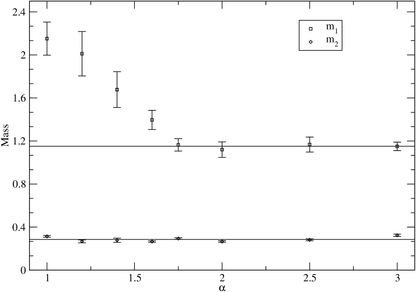
Figure 5: Values of the two mass parameters in eq. (16) as a function of $\alpha$. The light mass, $m_{2}$ is approximately constant at the value of $0.283(7)$, while the heavy mass initially decreases with increasing $\alpha$, reaching a constant value of $1.151(8)$.

In Fig. 4, we show the effective mass as a function of $x\,$for $\alpha=1$, $2$, and $3$. The solid lines are obtained from fits to the propagator using Eq. (16). The similarity to the other quenched models is quite clear. For small $\alpha$ there is an initial decrease and then rise of the effective mass, much like Fig. 2(c); as $\alpha$ increases, this minimum vanishes. We plot in Fig. 5 the best-fit values of $m_{1}$ and $m_{2}$ as a function of $\alpha$. Note that the behavior of $m_{2}$ is consistent with it being constant in this region, while $m_{1}$ appears to be decreasing to a constant limit as $\alpha$ increases.

Our results are roughly consistent with the work of Leinweber et al., who performed high-precision studies of the $SU(3)$ gluon propagator at $\alpha=\infty$.Leinweber:1998uu Among a large variety of possible functional forms for the gluon propagator, they found that their data was best fit by the functional form

$$G(k)=Z\left[\frac{AM^{2\delta}}{(k^{2}+M^{2})^{1+\delta}}+\frac{1}{k^{2}+M^{2}}L(k^{2},M)\right]\ ,$$ (17)

with $L(k^{2},M)$ an infrared-regulated version of the asymptotic behavior of the renormalized gluon propagator in the continuum. Their best fit was achieved with the parameters $\delta=2.2^{+0.1+0.2}_{-0.2-0.3}$, $M=(1020\pm 100\pm 25)\,\textrm{MeV}$, and $A=9.8^{+0.1}_{-0.9}$. Many other functional forms were ruled out.

Our results suggest that the lighter mass parameter $m_{2}$ is independent of $\alpha$, at least for large $\alpha$ (in the Higgs phase). If $m_{2}$ is indeed independent of gauge choice, as least within the class of covariant gauges considered, it seems natural to identify it as the gluon mass. As a consequence of the quenched character of lattice gauge fixing, this state partially mixes with another, heavier state, with a mass on the order of the scalar or vector glueball.Teper:1998kw

Note that the value of the lightest mass in the propagator may be difficult to extract from the effective mass. While it is true that the effective mass tends asymptotically to the lightest mass, the approach to the limit can be much slower than in a conventional field theory obeying spectral positivity. For example, at $\alpha=3.0$, $m_{eff}$ at $x=7$ is substantially lighter than $m_{2}$. Having a theoretical basis for the form of the propagator is crucial in estimating the mass.

Another application of lattice gauge fixing is Abelian projection, a method for investigating the confining properties of gauge theories. In lattice gauge theories, Abelian projection is implemented as an algorithm for extracting an ensemble of Abelian gauge field configurations from an ensemble of non-Abelian configurations. A notable success of lattice studies of Abelian projection Suzuki:1989gp ; Hioki:1991ai has been the correlation of the string tension of the projected theory with the string tension of the underlying non-Abelian theory.

These lattice studies of Abelian projection typically use gauge fixing in an integral way. Taking for clarity the case of $SU(2)$, the gauge fixing functional is

$$S_{gf}=\sum_{x,\mu}\frac{\alpha}{2}Tr\left[g\left(x\right)U_{\mu}\left(x\right)g^{+}\left(x+\mu\right)\sigma_{3}g\left(x+\mu\right)U_{\mu}^{+}\left(x\right)g^{+}\left(x\right)\sigma_{3}\right]\ ,$$ (18)

which is conventionally maximized over the gauge orbit, corresponding to the limit $\alpha\to\infty$ in the formalism used here. An initial study of the phase structure in the $SU(2)$ case finds evidence for a first order phase transition as $\alpha$ is varied at $\beta=2.4$.Mitrjushkin:2001hr The aim of this procedure is to transform an $SU(2)$ configuration into a gauge-equivalent one which lies mostly in a given $U(1)$ subgroup. After this gauge-fixing, the actual projection to $U(1)$ is performed.

In the case where no gauge fixing is done ($\alpha=0$), and only projection occurs, Faber et al. Faber:1998en and Ogilvie Ogilvie:1998wu have proved that the asymptotic string tension measured in the projected and underlying theories are the same. Furthermore, Ogilvie Ogilvie:1998wu has proven that this result should continue to hold for small $\alpha$, under the assumption that the gauge fixing does not violate spectral positivity. However, the fact that the string tension evaluated using various forms of Abelian projection with gauge fixing is consistently slightly different from the actual non-Abelian string tension Stack:2000kf ; Bornyakov:2000cd suggests that a violation of spectral positivity may indeed be occurring.

Figure 6: An example of a problematic diagram when calculating the expectaion value of Eq. (20). The solid line is the Wilson Loop, the dotted lines are $\phi$ propagators, and the wavy lines are gluons.

We identify the origin of this violation as the presence of a quenched scalar field. The case of $SU(2)$ is particularly clear. Note that the combination $g^{+}\left(x\right)\sigma_{3}g\left(x\right)$ occurring in $S_{gf}$ can be written as a Hermitian scalar field $\phi(x)$, where $\phi$ transforms as the adjoint representation of the gauge group. The field $\phi$ is traceless, $Tr(\phi)=0$, and satisfies $Tr(\phi^{2})=2$. The gauge fixing action is thus equivalent to an adjoint scalar action of the form

$$S_{gf}=\sum_{x,\mu}\frac{\alpha}{2}Tr\left[\phi\left(x\right)U_{\mu}\left(x\right)\phi\left(x+\mu\right)U_{\mu}^{+}\left(x\right)\right]\text{.}$$ (19)

As we have seen, such quenched fields naturally lead to violations of spectral positivity. Suppose we wish to measure a $U(1)$ projected Wilson loop. This may be obtained from the expectation value of

$$Tr\,\prod_{j}\frac{1}{2}(1+\sigma_{3})g_{j}U_{j}g^{+}_{j+1}=Tr\,\prod_{j}\frac{1}{2}(1+\phi_{j})U_{j}\ ,$$ (20)

where the product is ordered along a closed path labeled by the index $j$. The $U(1)$ projected loop is represented in the underlying quenched Higgs theory as a sum of Wilson loops with all possible insertions of $\phi$ at lattice sites on the path. When four or more $\phi$ fields are inserted, problematic subdiagrams appear of the type shown in Fig. 6. Such terms lead to a violation of spectral positivity: there are no internal $\phi$ loops in the quenched approximation, and an infinite set of diagrams occurring in the full, unquenched theory is omitted. This exactly parallels quenched QCD.

- (1) J. Greensite, [hep-lat/0301023].
- (2) J. Mandula and M. Ogilvie, Phys. Lett. B185 (1987) 127.
- (3) P. Coddington, A. Hey, J. Mandula and M. Ogilvie, Phys. Lett. B 197, 191 (1987).
- (4) J. E. Mandula, Phys. Rept. 315, 273 (1999).
- (5) M. F. Golterman, Pramana 45, S141 (1995) [hep-lat/9405002].
- (6) W. A. Bardeen, A. Duncan, E. Eichten, N. Isgur and H. Thacker, Nucl. Phys. Proc. Suppl. 106, 254 (2002) [hep-lat/0110187], Phys. Rev. D 65, 014509 (2002) [hep-lat/0106008].
- (7) D. Zwanziger, Nucl. Phys. B 345, 461 (1990).
- (8) C. Parrinello and G. Jona-Lasinio, Phys. Lett. B 251, 175 (1990).
- (9) S. Fachin and C. Parrinello, Phys. Rev. D 44, 2558 (1991).
- (10) L. Giusti, M. L. Paciello, C. Parrinello, S. Petrarca and B. Taglienti, Int. J. Mod. Phys. A 16, 3487 (2001) [hep-lat/0104012].
- (11) W. Bock, M. Golterman, M. Ogilvie and Y. Shamir, Phys. Rev. D 63, 034504 (2001) [hep-lat/0004017].
- (12) D. S. Henty,O. Oliveira, C. Parrinello and S. Ryan [UKQCD Collaboration], Phys. Rev. D 54, 6923 (1996) [hep-lat/9607014].
- (13) E. H. Fradkin and S. H. Shenker, Phys. Rev. D 19, 3682 (1979).
- (14) C. A. Aubin and M. C. Ogilvie, in preparation.
- (15) D. B. Leinweber, J. I. Skullerud, A. G. Williams and C. Parrinello [UKQCD Collaboration] Phys. Rev. D 60, 094507 (1999) [Erratum-ibid. D 61, 079901 (2000)] [hep-lat/9811027].
- (16) M. J. Teper, [hep-th/9812187.]
- (17) T. Suzuki and I. Yotsuyanagi, Phys. Rev. D 42, 4257 (1990).
- (18) S. Hioki, S. Kitahara, S. Kiura, Y. Matsubara, O. Miyamura, S. Ohno and T. Suzuki, Phys. Lett. B 272, 326 (1991) [Erratum-ibid. B 281, 416 (1992)].
- (19) V. K. Mitrjushkin and A. I. Veselov, JETP Lett. 74, 532 (2001) [Pisma Zh. Eksp. Teor. Fiz. 74, 605 (2001)] [arXiv:hep-lat/0110200].
- (20) M. Faber, J. Greensite and S. Olejnik, JHEP 9901, 008 (1999) [hep-lat/9810008].
- (21) M. C. Ogilvie, Phys. Rev. D 59, 074505 (1999) [hep-lat/9806018].
- (22) J. D. Stack and W. W. Tucker, Nucl. Phys. Proc. Suppl. 94, 529 (2001) [arXiv:hep-lat/0011034].
- (23) V. G. Bornyakov, D. A. Komarov, M. I. Polikarpov and A. I. Veselov, JETP Lett. 71, 231 (2000) [arXiv:hep-lat/0002017].