Nucleon axial charge from quenched lattice QCD with domain wall fermions

Abstract

We present a quenched lattice calculation of the nucleon isovector vector and axial-vector charges $g_{{}_{V}}$ and $g_{{}_{A}}$. The chiral symmetry of domain wall fermions makes the calculation of the nucleon axial charge particularly easy since the Ward-Takahashi identity requires the vector and axial-vector currents to have the same renormalization, up to lattice spacing errors of order ${\cal O}(a^{2})$. The DBW2 gauge action provides enhancement of the good chiral symmetry properties of domain wall fermions at larger lattice spacing than the conventional Wilson gauge action. Taking advantage of these methods and performing a high statistics simulation, we find a significant finite volume effect between the nucleon axial charges calculated on lattices with $(1.2\,{\rm fm})^{3}$ and $(2.4\,{\rm fm})^{3}$ volumes ($a\approx 0.15$ fm). On the large volume we find $g_{{}_{A}}=1.212\pm 0.027({\rm stat})\pm 0.024({\rm norm})$. The quoted systematic error is the dominant (known) one, corresponding to current renormalization. We discuss other possible remaining sources of error. This theoretical first principles calculation, which does not yet include isospin breaking effects, yields a value of $g_{{}_{A}}$ only a little bit below the experimental one, $1.2670\pm 0.0030$.

I Introduction

The axial charge $g_{{}_{A}}$ of the nucleon, or more precisely its ratio to the vector charge, $g_{{}_{V}}$, appears to be a good test of our understanding of the structure of the nucleon. First of all, it is very accurately measured from neutron $\beta$ decay, $g_{{}_{A}}/g_{{}_{V}}=1.2670\pm 0.0030$ Hagiwara:2002fs . And, among the nucleon form factors or moments of structure functions, it is technically the simplest from the point of view of a lattice QCD numerical calculation.

Four form factors appear in neutron $\beta$ decay: the vector and induced tensor form factors from the vector current,

$$\langle p|V^{+}_{\mu}(x)|n\rangle=\bar{u}_{p}[\gamma_{\mu}g_{{}_{V}}(q^{2})-q_{\lambda}\sigma_{\lambda\mu}g_{{}_{T}}(q^{2})]u_{n}e^{-iq\cdot x},$$ (1)

and the axial-vector and induced pseudo-scalar form factors from the axial-vector current,

$$\langle p|A^{+}_{\mu}(x)|n\rangle=\bar{u}_{p}[\gamma_{\mu}\gamma_{5}g_{{}_{A}}(q^{2})-iq_{\mu}\gamma_{5}g_{{}_{P}}(q^{2})]u_{n}e^{-iq\cdot x}.$$ (2)

Here $q=p_{n}-p_{p}$ is the momentum transfer between the proton ($p$) and neutron ($n$). In the limit $|{\vec{q}}|\rightarrow 0$, the momentum transfer should be small because the mass difference of the neutron and proton is only about 1.3 MeV. This makes the limit $q^{2}\rightarrow 0$, where the vector and axial-vector form factors dominate, a good approximation. Their values in this limit are called the vector and axial charges of the nucleon: $g_{{}_{V}}=g_{{}_{V}}(q^{2}=0)$ and $g_{{}_{A}}=g_{{}_{A}}(q^{2}=0)$. Experimentally, $g_{{}_{V}}=\cos\theta_{C}$ (with the Cabibbo mixing angle $\theta_{C}$), and $g_{{}_{A}}=1.2670(30)\times g_{{}_{V}}$.

Since they are defined at zero momentum transfer, a naive expectation is that $g_{{}_{V}}$ and $g_{{}_{A}}$ are easier to calculate on the lattice than form factors which require non-zero momentum transfer. Despite this, quenched QCD lattice calculations with Wilson fermions at finite lattice cutoff ($a^{-1}\sim 2$ GeV) have underestimated $g_{{}_{A}}$ by about 20%  Fukugita:1995fh ; Liu:1994ab ; Gockeler:1996wg (see Table 1 for a summary of previous calculations). This suggests systematic errors, which may arise from (1) the quenched approximation, (2) operator renormalization, (3) non-zero-lattice-spacing $a$ and loss of chiral symmetry for Wilson and Kogut-Susskind fermions, and (4) finite volume, remain in the lattice calculation.

The first three errors have been addressed in previous calculations. The SESAM and LHPC collaborations found that unquenching does not solve the problem as the estimated value $g_{{}_{A}}$ decreases by 5-10% Gusken:1999as ; Dolgov:2002zm . On the other hand, reducing the lattice spacing error seems to increase the value, but only by a small amount, $\mathrel{\hbox to0.0pt{\raise 2.20013pt\hbox{$<$}\hss}{\lower 2.20013pt\hbox{$\sim$}}}$ 5% Capitani:1999zd ; Horsley:2000pz . Perhaps more important is the calculation of the renormalization factor $Z_{{}_{A}}$ for the axial current. The one-loop perturbative renormalization factor, used in the case of Wilson fermions Fukugita:1995fh ; Liu:1994ab ; Gockeler:1996wg ; Dolgov:2002zm ; Gusken:1999as , was probably overestimated. The QCDSF-UKQCD collaboration reported that the non-perturbatively calculated renormalization factor ($Z_{{}_{A}}^{\rm nonpert}\sim 0.8$) is roughly 10% smaller than the one-loop one ($Z_{{}_{A}}^{\rm pert}\sim 0.9$) in the case of the non-perturbatively ${\cal O}(a)$ improved Wilson fermions Horsley:2000pz at $a^{-1}\sim 2-3$ GeV. Thus, the systematic error in the determination of the renormalization factor appears to be more important than the first two effects mentioned. The first two systematic errors listed above likely cannot resolve the issue that previous lattice calculations of $g_{{}_{A}}$ underestimate the experimental value.

The loss of chiral symmetry on the lattice is potentially significant. As is well known, $g_{{}_{A}}/g_{{}_{V}}=1$ in the absence of chiral symmetry breaking in QCD. Further, in the realistic case of spontaneously broken chiral symmetry, the ratio is still constrained by the axial Ward-Takahashi identity; $\partial_{\mu}A^{a}_{\mu}(x)=2mP^{a}(x)$. The Goldberger-Treiman relation derives from the nucleon matrix elements of the currents on both sides of this identity in the soft pion limit Goldberger:1958tr . We can easily understand the deviation of the ratio from unity in the context of the Gell-Mann-Oakes-Renner relation Gell-Mann:1968rz which is also related to the axial Ward-Takahashi identity. Thus, the explicit breaking of chiral symmetry at non-zero lattice spacing $a$ for Wilson fermions may induce significant errors which are only removed in the continuum limit.

In this work we use domain wall fermions (DWF), a fermion discretization scheme with almost perfectly preserved chiral symmetry Kaplan:1992bt ; Shamir:1993zy ; Narayanan:1993wx . This scheme introduces a fictitious fifth dimension in addition to the four dimensions of space-time. In the limit where the fifth-dimensional extent $L_{s}$ is taken to $\infty$, DWF preserve the axial Ward Takahashi identity Furman:1995ky at non-zero lattice spacing. With finite $L_{s}$ the suppression of explicit chiral symmetry breaking is effectively exponential in quenched simulations if the gauge field is sufficiently smooth Kikukawa:1999dk ; Hernandez:1998et ; Hernandez:2000iw ; Blum:2000kn ; AliKhan:2000iv ; Aoki:2002vt . This is always true if the lattice spacing is sufficiently small. In low energy cases like the one investigated here, the small breaking of the symmetry at finite $L_{s}$ is parametrized by a single universal “residual mass” parameter, $m_{\rm res}$, acting as an additive quark mass and which is defined from the axial Ward-Takahashi identity Blum:1998ud ; Blum:2000kn . Furthermore, the DWF scheme greatly simplifies the non-perturbative determination of the renormalization of quark bilinear currents Blum:2001sr . For example the renormalization factor of local vector and axial-vector current operators should be equal, $Z_{{}_{A}}=Z_{{}_{V}}$ Blum:2001sr . This means the ratio of the nucleon axial and vector charges calculated on the lattice directly yields the continuum value, ${\it i.e.}$ it is not renormalized Blum:2000cf ; Blum:2000cb . By employing the DWF scheme, the ambiguity in the renormalization of quark currents which may be present and problematic in other fermion discretization schemes is eliminated. We emphasize that the DWF calculation of the nucleon axial charge should not suffer from the systematic errors due to the operator renormalization and loss of chiral symmetry Blum:2000cf ; Blum:2000cb .

However, as is described in more detail in section III, in our first DWF calculation with the single-plaquette Wilson gauge action at $\beta=6.0$ and lattice volume $16^{3}\times 32\times 16$ (which correspond to $a^{-1}\approx 2$ GeV and spacial volume $\sim({\rm 1.6\,fm})^{3}$), we found that $g_{{}_{A}}$ exhibits a fairly strong dependence on the quark mass Blum:2000cb . A simple linear extrapolation of $g_{{}_{A}}$ to the chiral limit yielded a value that was almost a factor of two smaller than the experiment Blum:2000cb . This implied the presence of a large finite volume effect. To our surprise, we found no systematic study of such an effect in the literature. Note also that there is no volume dependence in the naive quark model Isgur:1979be nor in the MIT bag model Chodos:1974pn . In the former the ratio is determined by a simple spin-isospin algebra, and in the latter it arises from a simple overlap integral of the upper and lower component of the bag Dirac wave function.

To address the finite volume issue we need to have at the same time a sufficiently high lattice cutoff to preserve chiral symmetry reasonably well and at least two lattice volumes, preferably ones that are large compared to the charge radius of the proton. The Wilson gauge action will not work for this purpose since the chiral symmetry of DWF in the quenched case degrades rapidly as lattice spacing $a$ increases, while the computational cost necessitated by a very large lattice volume would be prohibitive. Fortunately various “renormalization-group-inspired” improved gauge actions preserve the chiral symmetry of DWF well while not demanding a large cutoff AliKhan:2000iv ; Aoki:2002vt . Thus both requirements, chiral symmetry and large physical volume, can be met at reasonable computational cost. Of the relatively well-established candidates in this class of improved gauge actions, we choose the “doubly-blocked Wilson 2 (DBW2)” action Takaishi:1996xj ; Aoki:2002vt .

The rest of this paper is organized as follows: in section II the lattice method for calculating $g_{{}_{A}}/g_{{}_{V}}$ is described. In section III the numerical results obtained for both Wilson and DBW2 actions are described in detail. Finally, in section IV we summarize the present work and discuss future directions.

II General Analytic Framework

II.1 The vector and axial charges

As mentioned in the introduction, four form factors are needed to describe neutron $\beta$ decay: the vector and induced tensor form factors for the vector current,

$$\langle p|V^{+}_{\mu}(0)|n\rangle=\bar{u}_{p}[\gamma_{\mu}g_{{}_{V}}(q^{2})-q_{\lambda}\sigma_{\lambda\mu}g_{{}_{T}}(q^{2})]u_{n},$$ (3)

and the axial and induced pseudo-scalar for the axial current,

$$\langle p|A^{+}_{\mu}(0)|n\rangle=\bar{u}_{p}[\gamma_{\mu}\gamma_{5}g_{{}_{A}}(q^{2})-iq_{\mu}\gamma_{5}g_{{}_{P}}(q^{2})]u_{n}.$$ (4)

The right hand side of each is the most general form consistent with Lorentz covariance. The momentum transfer $q=p_{n}-p_{p}$ becomes very small in the forward limit because of the small mass difference between the neutron and proton. In the limit $q^{2}\to 0$, which we take in this work, the vector and axial form factors dominate the matrix elements. We are neglecting the mass difference of the neutron and proton, and hence that of up and down quarks (we also neglect the electromagnetic mass difference.) For zero quark mass $m=m_{u}=m_{d}=0$ the action is symmetric under global chiral $SU(2)\times SU(2)$ flavor rotations acting on the quark fields. If $m\neq 0$, the symmetry is broken down to the vector (flavor) $SU(2)$ sub-group, and the associated vector charge, $g_{{}_{V}}$ is still conserved ($g_{{}_{V}}=1$). This situation is sometimes called CVC, conserved vector current. In the real world even this symmetry is softly broken by the small mass difference between up and down quarks, $m_{u}-m_{d}$. The explicit violation of the axial-vector symmetry by non-zero quark mass is sometimes called PCAC, or partially conserved axial-vector current. As is well known the axial $SU(2)$ symmetry is also spontaneously broken. Thus, the axial charge may in general deviate from unity, $g_{A}\neq 1$.

If the vector symmetry is preserved, a simple exercise in $SU(2)$ Lie algebra leads to the following (see Appendix A):

$$\langle p|A_{\mu}^{+}|n\rangle=2\langle p|A_{\mu}^{3}|p\rangle\\ =\langle p|A_{\mu}^{u}|p\rangle-\langle p|A_{\mu}^{d}|p\rangle$$

where $A_{\mu}^{+}={\bar{u}}\gamma_{\mu}\gamma_{5}d$, $A_{\mu}^{3}=\frac{1}{2}(A_{\mu}^{u}-A_{\mu}^{d})$, $A_{\mu}^{u}={\bar{u}}\gamma_{\mu}\gamma_{5}u$ and $A_{\mu}^{d}={\bar{d}}\gamma_{\mu}\gamma_{5}d$. $u$ and $d$ stand for the up and down quark fields. A similar relation holds for the vector case,

$$\langle p|V_{\mu}^{+}|n\rangle=2\langle p|V_{\mu}^{3}|p\rangle\\ =\langle p|V_{\mu}^{u}|p\rangle-\langle p|V_{\mu}^{d}|p\rangle$$

where $V_{\mu}^{+}={\bar{u}}\gamma_{\mu}d$, $V_{\mu}^{3}=\frac{1}{2}(V_{\mu}^{u}-V_{\mu}^{d})$, $V_{\mu}^{u}={\bar{u}}\gamma_{\mu}u$ and $V_{\mu}^{d}={\bar{d}}\gamma_{\mu}d$. The isovector vector charge $g_{{}_{V}}$ and the isovector axial charge $g_{{}_{A}}$ are defined by the strength of the right-hand side of Eqs. II.1 and II.1 in the forward limit ($q^{2}\rightarrow 0$). In addition, the polarized quark distributions in the proton for each flavor $f$, $\Delta\psi_{f}$, are defined by the forward matrix element of the flavor axial-vector currents $A_{\mu}^{f}$:

$$\left\langle k,s\left|\bar{\psi}_{f}\gamma_{\mu}\gamma_{5}\psi_{f}\right|k,s\right\rangle=\Delta\psi_{f}{\bar{u}}_{p}(k,s)\gamma_{\mu}\gamma_{5}u_{p}(k,s)$$ (5)

where $k$ and $s$ are proton four momentum and polarization. From CVC we find the relation $g_{{}_{A}}=\Delta u-\Delta d$.

Now consider the conserved electromagnetic current $j_{\mu}^{em}$ expressed in terms of the flavor vector currents $V^{f}_{\mu}$:

$$j_{\mu}^{em}=\sum_{f}Q_{f}V_{\mu}^{f}=\frac{2}{3}V_{\mu}^{u}-\frac{1}{3}V_{\mu}^{d}+\cdots\;\;.$$ (6)

Here $Q_{f}$ denotes the charge (in units of proton charge $e$) for a quark of flavor $f$, and the ellipsis denote possible flavors of heavier quarks which we henceforth ignore. Since the corresponding electromagnetic $U(1)$ gauge symmetry assures conservation of electric charge, for the neutron we find

$$\lim_{q^{2}\rightarrow 0}\langle n|j_{\mu}^{em}|n\rangle=0.$$ (7)

It follows that

$$\lim_{q^{2}\rightarrow 0}\langle n|V_{\mu}^{d}|n\rangle=2\times\lim_{q^{2}\rightarrow 0}\langle n|V_{\mu}^{u}|n\rangle.$$ (8)

On the other hand, under the assumption of CVC we have the following:

$$\langle n|V_{\mu}^{u}|n\rangle = \langle p|V_{\mu}^{d}|p\rangle$$ (9)

$$\langle n|V_{\mu}^{d}|n\rangle = \langle p|V_{\mu}^{u}|p\rangle.$$ (10)

Thus we reach the following relation:

$$\lim_{q^{2}\rightarrow 0}\langle p|j_{\mu}^{em}|p\rangle=\lim_{q^{2}\rightarrow 0}\langle p|V_{\mu}^{d}|p\rangle=\lim_{q^{2}\rightarrow 0}\langle p|V_{\mu}^{u}-V_{\mu}^{d}|p\rangle.$$ (11)

Likewise, it follows that the vector charge, $g_{{}_{V}}$, must be unity (in units of $\cos\theta_{C}$ and $e$) under CVC since the proton electric charge is unity. As already mentioned, we expect a very small breaking from CVC because of the physical up and down quark mass difference. In the axial case, we expect non-conservation of $g_{{}_{A}}$ due to the small but non-zero up and down quark masses as well as the spontaneous breakdown of chiral symmetry.

II.2 Nucleon matrix elements

In this subsection we describe our method of lattice numerical calculation of the axial and vector charges of the nucleon. Hadronic matrix elements calculated on the lattice are determined from ratios of the relevant three-point to two-point correlation functions. Since the charges are defined at zero-momentum transfer, we do not have to introduce non-zero momentum projection for the nucleon source and sink for these correlation functions, nor for the current insertion. On the other hand since we are dealing with a spin-1/2 baryon, both correlation functions possess non-trivial Dirac spinor structure, so appropriate projections are necessary.

The zero-momentum two-point function for the nucleon is given by the sum over all spatial coordinates, $\vec{x}$,

$$\langle{\cal N}(t){\overline{\cal N}}(0)\rangle_{\alpha\beta}=\sum_{\vec{x}}\langle 0|{\cal N}_{\alpha}({\vec{x}},t){\overline{\cal N}}_{\beta}({\vec{0}},0)|0\rangle$$ (12)

where ${\cal N}(\vec{x},t)$ can be any operator with the same quantum numbers as the nucleon, namely unit baryon number, $J^{P}=(1/2)^{+}$, and isospin doublet. $\alpha$ and $\beta$ denote Dirac indices. Color and flavor indices are suppressed in the following unless noted otherwise. The two-point correlation has the asymptotic form

$$\langle{\cal N}(t){\overline{\cal N}}(0)\rangle_{\alpha\beta}=\frac{A_{{}_{N}}}{2}[1+{\rm sgn}(t)\gamma_{4}]_{\alpha\beta}e^{-M_{N}|t|}$$ (13)

at large Euclidean time, $t$. Here $M_{N}$ denotes the ground state mass of the nucleon. The amplitude $A_{{}_{N}}$ is defined as $\langle 0|{\cal N}(0)|N\rangle=\sqrt{A_{{}_{N}}}u_{N}$. In general, the baryon two-point function receives contribution from both positive and negative-parity states. By taking the trace with a projection operator $P_{+}=(1+\gamma_{4})/2$, we eliminate contributions from the opposite-parity state in forward time direction. Details of the parity projection are described in Sasaki:2001nf . Let us abbreviate the notation for the two-point function of the particle contribution from the desired (positive-parity) state as

$$G_{{}_{N}}(t)=\frac{1}{4}{\rm Tr}[P_{+}\langle{\cal N}(t){\overline{\cal N}}(0)\rangle].$$ (14)

The factor of 1/4 is our choice of normalization. At large $t$ this asymptotically approaches a simple exponential,

$$G_{{}_{N}}(t)\sim\exp(-M_{N}t).$$ (15)

For the proton, a standard choice for the interpolating operator is

$${\cal N}(x)=\varepsilon_{abc}[u_{a}^{T}(x)C\gamma_{5}d_{b}(x)]u_{c}(x)$$ (16)

where $C$ is the charge conjugation matrix defined as $C=\gamma_{4}\gamma_{2}$, $abc$ the color indices, $u$ and $d$ the up and down quark fields.

Next, let us define the zero-momentum three-point correlation function for quark bilinears, ${{\cal O}_{\Gamma}^{(f)}}(x)={\bar{\psi}}_{{}_{f}}(x)\Gamma\psi_{{}_{f}}(x)$:

$$\langle{\cal N}(t){{\cal O}_{\Gamma}}(t^{\prime}){\overline{\cal N}}(0)\rangle_{\alpha\beta}=\sum_{\vec{x}}\sum_{\vec{x}^{\prime}}\langle 0|T\{{\cal N}_{\alpha}({\vec{x}},t){\cal O}_{\Gamma}({\vec{x}}^{\prime},t^{\prime}){\overline{\cal N}}_{\beta}({\vec{0}},0)\}|0\rangle$$ (17)

where $\Gamma$ is any of the sixteen possible matrices in the Clifford algebra defined by the Dirac gamma matrices. When $t\gg t^{\prime}\gg 0$, the particle contribution of the zero-momentum three-point function becomes

$$\langle{\cal N}(t){{\cal O}_{\Gamma}}(t^{\prime}){\overline{\cal N}}(0)\rangle_{\alpha\beta}\rightarrow A_{{}_{N}}\lim_{q^{2}\rightarrow 0}g_{{}_{\Gamma}}(q^{2})\exp(-M_{N}t)(P_{+}\Gamma P_{+})_{\alpha\beta}.$$ (18)

Note two important points: first, the three-point function vanishes for $\Gamma$ other than 1, $\gamma_{4}$, $\gamma_{i}\gamma_{5}$ ($i=1$, 2, 3), and $\sigma_{ij}$ ($i,j=1$, 2, 3) because $P_{+}\Gamma P_{+}=0$ for $\Gamma$’s that do not commute with $\gamma_{4}$. Second, the r.h.s. of the above asymptotic formula does not depend on the insertion point of the operator ${\cal O}_{\Gamma}$. Any $t^{\prime}$-dependence arises from excited state contamination, i.e. away from the asymptotic regime.

In this paper, we calculate the isovector (quark-flavored) vector charge $g_{{}_{V}}$ and the isovector axial charge $g_{{}_{A}}$ of the nucleon. We define the spin projected three-point function for the relevant components of the vector current $V_{\mu}^{f}={\bar{\psi}}_{f}\gamma_{\mu}{\psi}_{f}$ and the axial current $A_{\mu}^{f}={\bar{\psi}}_{f}\gamma_{\mu}\gamma_{5}{\psi}_{f}$ by taking traces with the projection operators $P_{\Gamma}=P_{+}\Gamma^{-1}$:

$$G_{V}^{f}(t,t^{\prime}) = \frac{1}{4}{\rm Tr}[P_{V}\langle{\cal N}(t)V_{4}^{f}(t^{\prime}){\overline{\cal N}}(0)\rangle]$$ (19)

$$G_{A}^{f}(t,t^{\prime}) = \frac{1}{4}{\rm Tr}[P_{A_{i}}\langle{\cal N}(t)A_{i}^{f}(t^{\prime}){\overline{\cal N}}(0)\rangle]$$ (20)

where $P_{V}=P_{+}$ and $P_{A_{i}}=P_{+}\gamma_{i}\gamma_{5}$ ($i=1$, 2, 3). In order to extract $g_{{}_{\Gamma}}$ ($\Gamma$ is either $V$ or $A$) on the lattice, we have to identify a plateau in the ratio of the three- and two-point functions,

$$g_{{}_{\Gamma}}^{\rm lattice}={{G_{{}_{\Gamma}}^{u}(t,t^{\prime})-G_{{}_{\Gamma}}^{d}(t,t^{\prime})}\over{G_{{}_{N}}(t)}}$$ (21)

in the range of $t>t^{\prime}$ with fixed $t=t_{\rm sink}-t_{\rm source}$.

In general, lattice operators receive finite renormalizations relative to their continuum counterparts since the exact symmetries of the continuum are usually realized only in the continuum limit, $a\to 0$. Thus

$$g_{{}_{\Gamma}}^{\rm ren}=Z_{{}_{\Gamma}}g_{{}_{\Gamma}}^{\rm lattice}$$ (22)

requires some independent estimation of $Z_{{}_{\Gamma}}$, the renormalization of the quark bilinear currents,

$$[{\bar{\psi}}\Gamma\psi]^{\rm ren}=Z_{{}_{\Gamma}}[{\bar{\psi}}\Gamma\psi]^{\rm lattice}.$$ (23)

Since DWF possess full chiral symmetry at non-zero lattice spacing, a lattice conserved vector current ${\cal V}_{\mu}$ and partially-conserved axial-vector current ${\cal A}_{\mu}$ which receive no lattice renormalization can be defined, namely $Z_{{}_{\cal V}}$=$Z_{{}_{\cal A}}$=1 Furman:1995ky . However these conserved currents are point-split and require sums over the extra 5th dimension of DWF, so they are somewhat costly to work with in practice. Alternatively the local currents $V_{\mu}$ and $A_{\mu}$ which are naive transcriptions of the continuum operators are easier to deal with but receive a finite renormalization since they do not correspond to an exact symmetry of the action. However, the Ward-Takahashi identity satisfied by both types of currents is enough to ensure that the lattice renormalizations of the local currents are equal, $Z_{{}_{V}}=Z_{{}_{A}}$, up to terms of order ${\cal O}(a^{2})$ in the chiral limit and neglecting explicit chiral symmetry breaking for DWF at finite $L_{s}$.

$$\left(\frac{g_{{}_{A}}}{g_{{}_{V}}}\right)^{\rm ren}=\left(\frac{G_{{}_{A}}^{u}(t,t^{\prime})-G_{{}_{A}}^{d}(t,t^{\prime})}{G_{{}_{V}}^{u}(t,t^{\prime})-G_{{}_{V}}^{d}(t,t^{\prime})}\right)^{\rm lattice}+{\cal O}(a^{2}).$$ (24)

Note that the vector charge computed from the local current provides an independent estimate of $Z_{{}_{V}}$ since the renormalization of an operator does not depend on any particular matrix element and the renormalized, or physical, value of $g_{{}_{V}}$ is 1 by CVC.

$$Z_{{}_{V}}={{G_{{}_{N}}(t)}\over{{G_{{}_{{}_{V}}}^{u}(t,t^{\prime})-G_{{}_{{}_{V}}}^{d}(t,t^{\prime})}}}.$$ (25)

Comparison of $Z_{{}_{V}}$ thus obtained to the value of $Z_{{}_{A}}$ from the relation Blum:2000kn ,

$$\langle{\cal A}_{{}_{\mu}}(t)[\bar{\psi}\gamma_{5}\psi](0)\rangle=Z_{{}_{A}}\langle A_{\mu}(t)[\bar{\psi}\gamma_{5}\psi](0)\rangle,$$ (26)

yields an estimate of the ${\cal O}(a^{2})$ systematic errors arising from the method described here. These are discussed in section III.

Next we describe the particular interpolating operators, or quark sources and sinks, used to calculate lattice correlation functions. In our earlier work we used so-called wall-wall correlation functions constructed with quark sources generated from a unit source at each spatial site on a fixed source time-slice and summed over all spatial sites at the sink time-slice. Since the wall source or sink is gauge variant, we fix to the Coulmob gauge. Later we switched to wall-point correlation functions since they yield smaller statistical errors. For three point functions this approach is implemented with a sequential source. We discuss both types of correlation functions in turn.

First, we introduce the forward quark propagators from a wall source to a wall sink and from a wall source to a point sink, which may be written with the gauge fixed point-to-point quark propagator $S_{{}_{PP}}$:

$${S_{{}_{WW}}}(t,t^{\prime})^{ab}_{\alpha\beta} = \sum_{{\vec{x}}}{S_{{}_{PW}}}({\vec{x}},t;t^{\prime})^{ab}_{\alpha\beta},$$ (27)

$${S_{{}_{PW}}}({\vec{x}},t;t^{\prime})^{ab}_{\alpha\beta} = \sum_{{\vec{y}}}{S_{{}_{PP}}}({\vec{x}},t;{\vec{y}},t^{\prime})^{ab}_{\alpha\beta}$$ (28)

where the subscripts and superscripts denote Dirac and color indices, respectively. The quark three-point function resulting from insertion of the quark bilinear operator ${\bar{\psi}}_{f}\Gamma\psi_{f}$ is defined as

$${{\cal S}_{{}_{\Gamma}}}(t,t^{\prime},t^{\prime\prime})^{ab}_{\alpha\beta} = \sum_{{\vec{x}},{\vec{y}},{\vec{z}}}{S_{{}_{PP}}}({\vec{x}},t;{\vec{y}},t^{\prime})^{ac}_{\alpha\gamma}(\Gamma)_{\gamma\gamma^{\prime}}{S_{{}_{PP}}}({\vec{y}},t^{\prime};{\vec{z}},t^{\prime\prime})^{cb}_{\gamma^{\prime}\beta}$$ (29)

$$= \sum_{{\vec{z}}}\gamma_{5,\gamma\delta^{\prime}}{S_{{}_{PW}}^{*}}({\vec{x}},t^{\prime};t)^{ca}_{\delta^{\prime}\delta}\gamma_{5,\delta\alpha}(\Gamma)_{\gamma\gamma^{\prime}}{S_{{}_{PW}}}({\vec{x}},t^{\prime};t^{\prime\prime})^{cb}_{\gamma^{\prime}\beta}$$

where the second line results from ${S_{{}_{PP}}}({\vec{x}},t;{\vec{y}},t^{\prime})=\gamma_{5}{S_{{}_{PP}}^{\dagger}}({\vec{y}},t^{\prime};{\vec{x}},t)\gamma_{5}$. Thus, ${\cal S}_{{}_{\Gamma}}(t,t^{\prime},t^{\prime\prime})$ is constructed by combining wall-to-point quark propagators generated from two different source time-slices $t$ and $t^{\prime\prime}$ at either end of the lattice with the operator inserted in between them.

The two-point function for the nucleon in Eq.(12) is expressed in terms of quark propagators as

$$\langle{\cal N}(t){\overline{\cal N}}(0)\rangle_{\alpha\alpha^{\prime}} = \varepsilon_{abc}\varepsilon_{a^{\prime}b^{\prime}c^{\prime}}(C\gamma_{5})_{\beta\gamma}{S_{{}_{WW}}^{(d)}}(t,0)^{cc^{\prime}}_{\gamma\gamma^{\prime}}(C\gamma_{5})_{\beta^{\prime}\gamma^{\prime}}$$

$$\times \left[{S_{{}_{WW}}^{(u)}}(t,0)^{aa^{\prime}}_{\alpha\alpha^{\prime}}{S_{{}_{WW}}^{(u)}}(t,0)^{bb^{\prime}}_{\beta\beta^{\prime}}+{S_{{}_{WW}}^{(u)}}(t,0)^{aa^{\prime}}_{\alpha\beta^{\prime}}{S_{{}_{WW}}^{(u)}}(t,0)^{bb^{\prime}}_{\beta\alpha^{\prime}}\right]$$

Following Ref. Woloshyn:1989ae , the three-point function in Eq.(17) is easily obtained from the two-point function by replacing the ordinary quark propagator by the operator inserted one, ${\cal S}_{{}_{\Gamma}}(t,t^{\prime},0)$. Inserting the d and u quark currents, we obtain

$$\langle{\cal N}(t){\cal O}^{(d)}_{\Gamma}(t^{\prime}){\overline{\cal N}}(0)\rangle_{\alpha\alpha^{\prime}} = \varepsilon_{abc}\varepsilon_{a^{\prime}b^{\prime}c^{\prime}}(C\gamma_{5})_{\beta\gamma}{{\cal S}_{{}_{\Gamma}}^{(d)}}(t,t^{\prime},0)^{cc^{\prime}}_{\gamma\gamma^{\prime}}(C\gamma_{5})_{\beta^{\prime}\gamma^{\prime}}$$

$$\times \left[{S_{{}_{WW}}^{(u)}}(t,0)^{aa^{\prime}}_{\alpha\alpha^{\prime}}{S_{{}_{WW}}^{(u)}}(t,0)^{bb^{\prime}}_{\beta\beta^{\prime}}+{S_{{}_{WW}}^{(u)}}(t,0)^{aa^{\prime}}_{\alpha\beta^{\prime}}{S_{{}_{WW}}^{(u)}}(t,0)^{bb^{\prime}}_{\beta\alpha^{\prime}}\right]$$

and

$$\langle{\cal N}(t){\cal O}^{(u)}_{\Gamma}(t^{\prime}){\overline{\cal N}}(0)\rangle_{\alpha\alpha^{\prime}} = \varepsilon_{abc}\varepsilon_{a^{\prime}b^{\prime}c^{\prime}}(C\gamma_{5})_{\beta\gamma}{S_{{}_{WW}}^{(d)}}(t,0)^{cc^{\prime}}_{\gamma\gamma^{\prime}}(C\gamma_{5})_{\beta^{\prime}\gamma^{\prime}}$$

$$\times \left[{{\cal S}_{{}_{\Gamma}}^{(u)}}(t,t^{\prime},0)^{aa^{\prime}}_{\alpha\alpha^{\prime}}{S_{{}_{WW}}^{(u)}}(t,0)^{bb^{\prime}}_{\beta\beta^{\prime}}+{{\cal S}_{{}_{\Gamma}}^{(u)}}(t,t^{\prime},0)^{aa^{\prime}}_{\alpha\beta^{\prime}}{S_{{}_{WW}}^{(u)}}(t,0)^{bb^{\prime}}_{\beta\alpha^{\prime}}\right.$$

$$\left.+{S_{{}_{WW}}^{(u)}}(t,0)^{aa^{\prime}}_{\alpha\alpha^{\prime}}{{\cal S}_{{}_{\Gamma}}^{(u)}}(t,t^{\prime},0)^{bb^{\prime}}_{\beta\beta^{\prime}}+{S_{{}_{WW}}^{(u)}}(t,0)^{aa^{\prime}}_{\alpha\beta^{\prime}}{{\cal S}_{{}_{\Gamma}}^{(u)}}(t,t^{\prime},0)^{bb^{\prime}}_{\beta\alpha^{\prime}}\right].$$

The nucleon three-point function is the sum of the up and down quark contributions. The spin projected three-point functions are obtained from Eqs.19 and 20.

To enhance the signal, a point sink is more desirable than an extended sink. The wall-point type of three-point functions is implemented using the so-called sequential source method Bernard:1985ss ; Martinelli:1989rr ; Dolgov:2002zm . In addition we use box source instead of wall source to enhance the coupling to the ground state:

$${S_{{}_{PB}}}({\vec{x}},t;t^{\prime})^{ab}_{\alpha\beta}=\sum_{0\leq{\vec{y}}\leq B}{S_{{}_{PP}}}({\vec{x}},t;{\vec{y}},t^{\prime})^{ab}_{\alpha\beta}$$ (33)

We adjust the box size $B$ to about 1 fm. In describing the construction of the sequential source, it is convenient to introduce the “diquark” propagators:

$$\bm{\mathcal{D}}_{\alpha\alpha^{\prime}}({\vec{y}},t;0)_{\beta^{\prime}\beta}^{a^{\prime}a} = \varepsilon_{abc}\varepsilon_{a^{\prime}b^{\prime}c^{\prime}}(C\gamma_{5})_{\delta\beta}(C\gamma_{5})_{\delta^{\prime}\beta^{\prime}}$$ (34)

$$\times \left[{S_{{}_{PB}}^{(u)}}({\vec{y}},t;0)^{bb^{\prime}}_{\beta\beta^{\prime}}{S_{{}_{PB}}^{(u)}}({\vec{y}},t;0)^{cc^{\prime}}_{\gamma\gamma^{\prime}}+{S_{{}_{PB}}^{(u)}}({\vec{y}},t;0)^{bb^{\prime}}_{\gamma\beta^{\prime}}{S_{{}_{PB}}^{(u)}}({\vec{y}},t;0)^{cc^{\prime}}_{\beta\gamma^{\prime}}\right]$$

and

$$\bm{\mathcal{U}}_{\alpha\alpha^{\prime}}({\vec{y}},t;0)_{\beta^{\prime}\beta}^{b^{\prime}b} = \varepsilon_{abc}\varepsilon_{a^{\prime}b^{\prime}c^{\prime}}{S_{{}_{PB}}^{(d)}}({\vec{y}},t;0)^{cc^{\prime}}_{\gamma\gamma^{\prime}}$$

$$\times \left[(C\gamma_{5})_{\beta\gamma}(C\gamma_{5})_{\beta^{\prime}\gamma^{\prime}}{S_{{}_{PB}}^{(u)}}({\vec{y}},t;0)^{aa^{\prime}}_{\alpha\alpha^{\prime}}+(C\gamma_{5})_{\delta\gamma}(C\gamma_{5})_{\delta^{\prime}\gamma^{\prime}}{S_{{}_{PB}}^{(u)}}({\vec{y}},t;0)^{aa^{\prime}}_{\delta\delta^{\prime}}\delta_{\alpha\beta}\delta_{\alpha^{\prime}\beta^{\prime}}\right.$$

$$+ \left.(C\gamma_{5})_{\beta\gamma}(C\gamma_{5})_{\delta^{\prime}\gamma^{\prime}}{S_{{}_{PB}}^{(u)}}({\vec{y}},t;0)^{aa^{\prime}}_{\alpha\delta^{\prime}}\delta_{\alpha^{\prime}\beta^{\prime}}+(C\gamma_{5})_{\delta\gamma}(C\gamma_{5})_{\beta^{\prime}\gamma^{\prime}}{S_{{}_{PB}}^{(u)}}({\vec{y}},t;0)^{aa^{\prime}}_{\delta\alpha^{\prime}}\delta_{\alpha\beta}\right].$$

The “down diquark” ($\cal D$) and “up diquark” ($\cal U$) are defined by the down quark removed propagator and one up quark removed propagator from the nucleon two-point function. Now using the diquark we can reconstruct the point-to-wall type of the nucleon two-point function as

$$\langle{\cal N}(t){\overline{\cal N}}(0)\rangle_{\alpha\alpha^{\prime}}=\sum_{\vec{y}}\bm{\mathcal{D}}_{\alpha\alpha^{\prime}}({\vec{y}},t;0)_{\beta^{\prime}\beta}^{ba}{S_{{}_{PB}}^{(d)}}({\vec{y}},t;0)^{ab}_{\beta\beta^{\prime}}=\frac{1}{2}\sum_{\vec{y}}\bm{\mathcal{U}}_{\alpha\alpha^{\prime}}({\vec{y}},t;0)_{\beta^{\prime}\beta}^{ba}{S_{{}_{PB}}^{(u)}}({\vec{y}},t;0)^{ab}_{\beta\beta^{\prime}}.$$ (36)

In terms of the diquarks the three-point functions of an arbitrary quark bilinear operator ${\bar{\psi}}_{f}\Gamma\psi_{f}$ at a location $({\vec{z}},t^{\prime})$ can be written for the down quark

$$\langle{\cal N}(t){\cal O}^{(d)}_{\Gamma}(t^{\prime}){\overline{\cal N}}(0)\rangle_{\alpha\alpha^{\prime}}=\sum_{{\vec{y}},{\vec{z}}}\bm{\mathcal{D}}_{\alpha\alpha^{\prime}}({\vec{y}},t;0)_{\beta^{\prime}\beta}^{a^{\prime}a}{S_{{}_{PP}}^{(d)}}({\vec{y}},t;{\vec{z}},t^{\prime})^{ae}_{\beta\delta}(\Gamma)_{\delta\delta^{\prime}}{S_{{}_{PB}}^{(d)}}({\vec{z}},t^{\prime};0)^{ea^{\prime}}_{\delta^{\prime}\beta^{\prime}}$$ (37)

and for the up quark

$$\langle{\cal N}(t){\cal O}^{(u)}_{\Gamma}(t^{\prime}){\overline{\cal N}}(0)\rangle_{\alpha\alpha^{\prime}}=\sum_{{\vec{y}},{\vec{z}}}\bm{\mathcal{U}}_{\alpha\alpha^{\prime}}({\vec{y}},t;0)_{\beta^{\prime}\beta}^{b^{\prime}b}{S_{{}_{PP}}^{(u)}}({\vec{y}},t;{\vec{z}},t^{\prime})^{be}_{\beta\delta}(\Gamma)_{\delta\delta^{\prime}}{S_{{}_{PB}}^{(u)}}({\vec{z}},t^{\prime};0)^{eb^{\prime}}_{\delta^{\prime}\beta^{\prime}}.$$ (38)

For the construction of the three point functions we need the backward propagators from the sink point $({\vec{y}},t)$ to the operator insertion point $({\vec{z}},t^{\prime})$. However, it is highly expensive to prepare the required point-to-point quark propagators from all points $(\vec{y},t)$. This difficulty is easily circumvented by directly computing the generalized quark propagators $\bm{\mathcal{D}}_{\alpha\alpha^{\prime}}({\vec{y}},t;0){S_{{}_{PP}}^{(d)}}({\vec{y}},t;{\vec{z}},t^{\prime})$ and $\bm{\mathcal{U}}_{\alpha\alpha^{\prime}}({\vec{y}},t;0){S_{{}_{PP}}^{(u)}}({\vec{y}},t;{\vec{z}},t^{\prime})$ with the sequential source method.

Before describing details of the sequential source propagator, we should apply the spin projection $P_{\Gamma}$ to diquarks in order to reduce the cost from having to calculate all $4\times 4$ matrices for external spinor indices ($\alpha,\alpha^{\prime}$). In this article, we only need two kinds of spin projections, i.e. $P_{V}$ and $P_{A_{3}}$ so that it reduces the amount of calculations by a factor of eight in comparison with the unprojected case. The spin projected source for a down quark insertion is

$$\bm{\Phi}_{d}({\vec{y}},t;0)^{ab}_{\alpha\beta}=\frac{1}{4}\bm{\mathcal{D}}_{\gamma\gamma^{\prime}}({\vec{y}},t;0)_{\alpha\beta}^{ab}(P_{\Gamma})_{\gamma^{\prime}\gamma},$$ (39)

and for the up quark

$$\bm{\Phi}_{u}({\vec{y}},t;0)^{ab}_{\alpha\beta}=\frac{1}{4}\bm{\mathcal{U}}_{\gamma\gamma^{\prime}}({\vec{y}},t;0)_{\alpha\beta}^{ab}(P_{\Gamma})_{\gamma^{\prime}\gamma}.$$ (40)

Finally, the sequential source down quark propagator is

$$\bm{\Sigma}_{d}(t,0;{\vec{z}},t^{\prime})^{ab}_{\alpha\beta}=\left(\sum_{{\vec{y}},t^{\prime\prime}}\gamma_{5,\beta\gamma}{S_{{}_{PP}}^{(d)}}({\vec{z}},t^{\prime};{\vec{y}},t)^{be}_{\gamma\gamma^{\prime}}\gamma_{5,\gamma^{\prime}\delta}\delta_{t^{\prime\prime},t}\bm{\Phi}^{\ast}_{d}({\vec{y}},t^{\prime\prime};0)^{ae}_{\alpha\delta}\right)^{*},$$ (41)

and the sequential source up quark propagator is

$$\bm{\Sigma}_{u}(t,0;{\vec{z}},t^{\prime})^{ab}_{\alpha\beta}=\left(\sum_{{\vec{y}},t^{\prime\prime}}\gamma_{5,\beta\gamma}{S_{{}_{PP}}^{(u)}}({\vec{z}},t^{\prime};{\vec{y}},t)^{be}_{\gamma\gamma^{\prime}}\gamma_{5,\gamma^{\prime}\delta}\delta_{t^{\prime\prime},t}\bm{\Phi}^{\ast}_{u}({\vec{y}},t^{\prime\prime};0)^{ae}_{\alpha\delta}\right)^{*}.$$ (42)

which may be calculated by solving the matrix equations

$$\sum_{{\vec{x}},t^{\prime\prime}}\bm{\Sigma}_{f}(t,0;{\vec{x}},t^{\prime\prime})^{ab}_{\alpha\beta}\;\;\bm{\mathcal{M}}^{\dagger}({\vec{x}},t^{\prime\prime};{\vec{z}},t^{\prime})_{\beta\gamma}^{bc}=\delta_{tt^{\prime}}\bm{\Phi}_{f}({\vec{z}},t^{\prime};0)^{ac}_{\alpha\gamma}$$ (43)

where $\bm{\mathcal{M}}$ is the Dirac matrix. Consequently, in terms of the sequential source propagator, the spin projected three point function for the down quark is written

$$G_{\Gamma}^{d}(t,t^{\prime})=\sum_{{\vec{z}}}\bm{\Sigma}_{d}(t,0;{\vec{z}},t^{\prime})^{ab}_{\alpha\beta}(\Gamma)_{\beta\gamma}{S_{{}_{PB}}^{(d)}}({\vec{z}},t^{\prime};0)^{ba}_{\gamma\alpha}$$ (44)

and for the up quark is

$$G_{\Gamma}^{u}(t,t^{\prime})=\sum_{{\vec{z}}}\bm{\Sigma}_{u}(t,0;{\vec{z}},t^{\prime})^{ab}_{\alpha\beta}(\Gamma)_{\beta\gamma}{S_{{}_{PB}}^{(u)}}({\vec{z}},t^{\prime};0)^{ba}_{\gamma\alpha}.$$ (45)

In the case of keeping the up and down quark masses equal, the total cost for computing the sequential source propagator is a factor of two over the cost for wall-wall correlation functions. However, the resulting box-point correlation functions yield smaller statistical errors.

III Numerical Results

We have performed quenched lattice calculations using two different gauge actions, the standard Wilson and the improved DBW2 Takaishi:1996xj . Details and some relevant results of both simulations are summarized in Tables II, 3, and 4. We describe the nucleon matrix element results for each one separately, then compare them and draw some conclusions.

III.1 Wilson gauge action results at $\beta=6.0$

We have performed a quenched simulation on a $16^{3}\times 32$ lattice with the standard single-plaquette Wilson action at $\beta=6/g^{2}=6.0$ which corresponds to a lattice cut-off of $a^{-1}=1.922$ GeV set by the $\rho$ mass Blum:2000kn . Quark propagators were generated with four bare masses, $m_{f}=$0.02, 0.03, 0.04 and 0.05, using DWF with $L_{s}=16$ and $M_{5}=1.8$. The nucleon matrix elements were averaged on a set of 400 gauge configurations. Hadron masses computed on these lattices are tabulated in Table 5. Preliminary results for the nucleon charges were first reported in Blum:2000cb .

We calculated wall-source quark propagators on each Coulomb-gauge-fixed configuration for both periodic and anti-periodic boundary conditions in the time direction for the quarks. A simple linear combination of these propagators then yields a forward (or backward) in time propagator. To compute the correlation functions, we employed the wall-wall method described in the previous section with source locations fixed at $t_{src}=5$ and $t^{\prime}_{src}=21$.

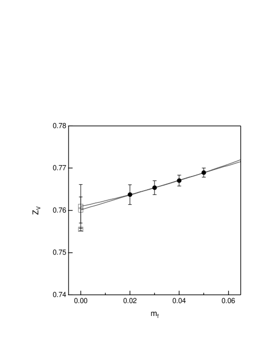
Figure 2: Quark mass dependence of the vector current renormalization, $Z_{{}_{V}}=1/g_{{}_{V}}^{\rm latt}$, Wilson gauge action (note scale). Lines denote uncorrelated linear and quadratic fits to the data points. Extrapolated values are consistent with the axial-vector current renormalization computed from meson two-point functions Blum:2000kn ; Blum:2001sr to less than a percent.

In Figure 1 we show the dependence of the vector renormalization, $Z_{{}_{V}}=1/g_{{}_{V}}^{\rm lattice}$ on the location of the current insertion. A good plateau is observed in the middle region between the source and sink. The quoted errors are estimated by a single elimination jack-knife method. The dashed lines represent the average value and statistical error in the time-slice range $5\leq t-t_{\rm src}\leq 11$. The mass dependence of $Z_{{}_{V}}$ is rather mild as seen in Figure 2 and given in Table 6. The values 0.7601(31) for a linear fit and 0.7610 (52) for a quadratic fit at $m_{f}=0$ agree well with $Z_{{}_{A}}=0.7555(3)$ Blum:2000kn , which was obtained from a calculation of meson two-point correlation functions. The discrepancy $\Delta Z\equiv|1-Z_{{}_{A}}/Z_{{}_{V}}|$ is less than 0.6% which implies the ${\cal O}(a^{2})$ error that remains after taking the $m_{f}\to 0$ limit is quite small.

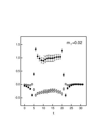
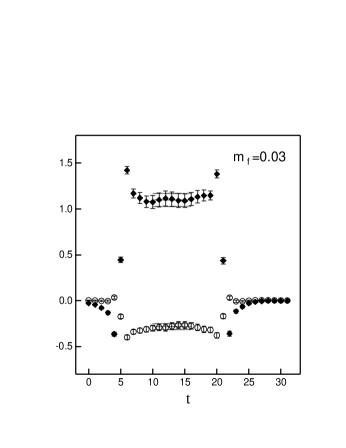
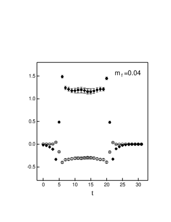
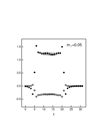
Figure 3: The lattice estimates of the spin-dependent densities $\Delta u$ (upper curves) and $\Delta d$ (lower curves) for the Wilson gauge action. Decent plateaus are observed for each quark mass. The lines denote central values and statistical errors from constant fits over the plateaus.

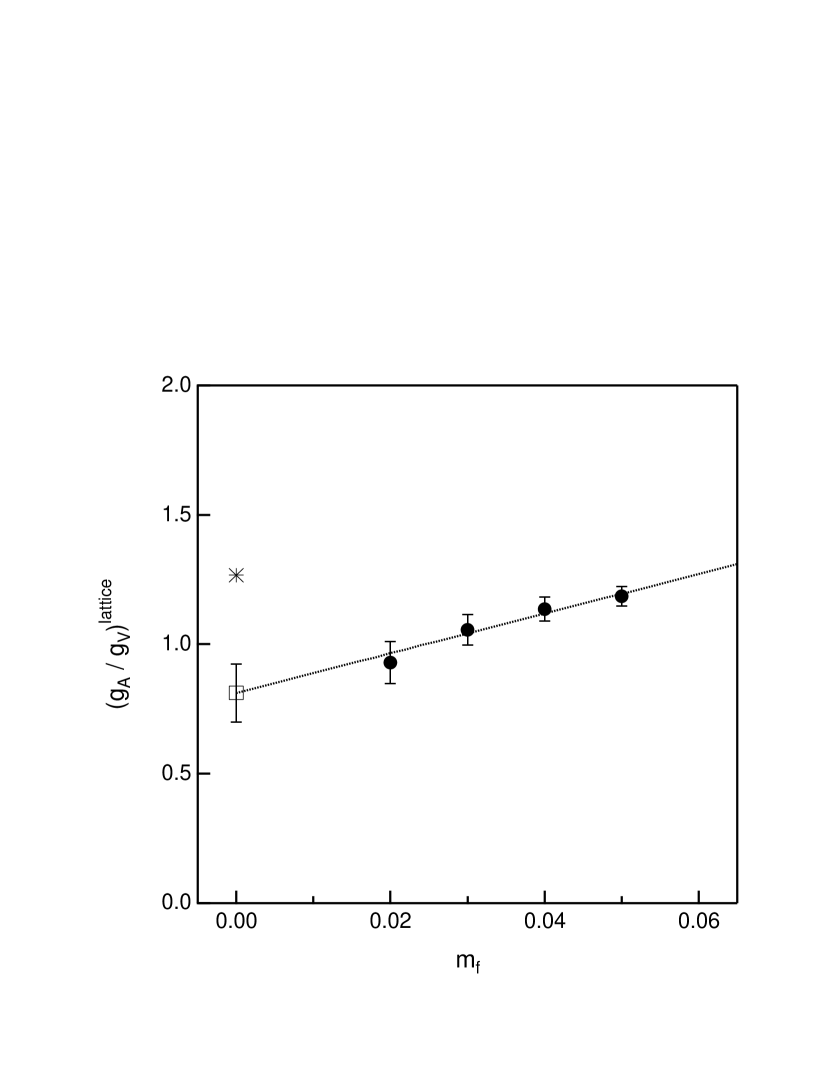
Figure 4: The ratio of nucleon charges $g_{{}_{A}}/g_{{}_{V}}$, Wilson gauge action, $V\approx$ (1.6 fm)³. A marked decrease towards the chiral limit is evident. A linear fit significantly underestimates the experimental value (burst).

As is seen in Figure 3, plateaus are evident for the spin-dependent distribution functions, $\Delta u$ and $\Delta d$, in the range $5\leq t-t_{\rm src}\leq 11$. Thus, we compute the charge ratios $(g_{{}_{A}}/g_{{}_{V}})^{\rm lattice}$ at each $m_{f}$ by taking a weighted average over this time slice range. In Figure 4 a strong dependence on $m_{f}$ appears. A simple linear extrapolation to $m_{f}=0$ yields $0.812(112)$, which is roughly 2/3 of the experimental value. However, a simple linear ansatz may not describe the data which show increasing downward curvature for lighter quark mass (note that the points are correlated in this quenched calculation since they are computed on the same gauge configurations). In general chiral logarithms may appear and were considered. In fact, the data are not compelling for such terms, arising in either quenched or full chiral perturbation theory Kim:1998bz ; Jenkins:1991es . The results for each mass are reproduced in Table 6.

This implies the existence of other systematic errors. As was mentioned in the introduction, a large systematic error in previous lattice calculations of $g_{{}_{A}}$ came from the determination of the renormalization constant $Z_{{}_{A}}$. As shown above using DWF, the value of $g_{{}_{A}}$ is determined in a fully nonperturbative way, with or without explicit renormalization. The systematic error stemming from the incomplete cancellation of renormalization factors in the ratio is less than 1% as we saw by comparing $Z_{{}_{V}}=1/g_{{}_{V}}^{\rm lattice}$ and $Z_{{}_{A}}$ calculated from meson two-point functions. In addition, comparing the chirally extrapolated values of $(g_{{}_{A}}/g_{{}_{V}})^{\rm lattice}$ and $Z_{{}_{A}}g_{{}_{A}}^{\rm lattice}$ leads to an even smaller error, although it relies on the linear extrapolation which was not very compelling. Another possible systematic error is the contribution of excited states, the presence or absence of which was checked by slightly enlarging the separation between wall sources, $t_{\rm src}(=5)$ and $t_{\rm sink}(=27)$. While the larger separation induces more noise in the signal, the central value of $g_{{}_{A}}$ is essentially unchanged for each quark mass; thus we cannot detect a systematic effect outside of the statistical errors. Still, this source of error appears to be small.

Detailed detection of quenching effects: quenched chiral logarithms, unsuppressed fermionic zero modes, and the absence of the physical pion cloud, is beyond our scope at present since these require very light quark masses and correspondingly large statistics. Thus, by process of elimination we are lead to focus on finite volume effects which we discuss in the next section. The volume employed for the calculations in this subsection is roughly $(1.5-1.6\,{\rm fm})^{3}$ which can barely accommodate a proton with mean square radius estimated to be about 0.8 fm Hagiwara:2002fs .

III.2 DBW2 action results at $\beta=0.87$

To determine $g_{{}_{A}}$ in a large physical volume, say $\mathrel{\hbox to0.0pt{\raise 2.20013pt\hbox{$>$}\hss}{\lower 2.20013pt\hbox{$\sim$}}}(2{\rm\,fm})^{3}$, we have performed a DWF simulation on a lattice with larger spacing. In general, it is difficult to maintain the good chiral properties of DWF as $a$ increases at fixed $L_{s}$, especially with the Wilson gauge action Blum:2000kn ; AliKhan:2000iv . It has been shown that the Iwasaki gauge action enables studies of quenched DWF with smaller $L_{s}$ than the Wilson gauge action Wu:1999cd ; AliKhan:2000iv . Recent quenched studies by the RBC collaboration have shown that the chiral symmetry of DWF are even better with a similar type of renormalization group improved gauge action, DBW2 Aoki:2002vt . The chiral symmetry of DWF with DBW2 is significantly improved over the Iwasaki action. A very small additive quark mass $m_{\rm res}\sim 0.8$ MeV is achieved on a lattice with $a^{-1}\approx 1.3$ GeV and $L_{s}=16$. Good scaling behavior of the light hadron spectrum is observed as well Aoki:2002vt .

To study finite volume effects numerical simulations were performed at $\beta=0.87$ ($a\approx 0.15$ fm) on two lattice sizes, $8^{3}\times 24$ and $16^{3}\times 32$, with $L_{s}=16$ and $M_{5}=1.8$. Our results are analyzed on 400 quenched gauge configurations for the smaller lattice ($La\sim 1.2\,{\rm fm}$) and 416 configurations for the larger lattice ($La\sim 2.4\,{\rm fm}$). Hadron masses computed in this calculation are summarized in Table 7. Meson masses ($m_{\pi}$ and $m_{\rho})$ for the $16^{3}\times 32$ lattice are evaluated from 100 configurations.

In this calculation, we utilize the sequential quark propagator method to compute three-point functions as described in section II. We checked for consistency with the wall-wall method on the smaller $8^{3}\times 24$ lattice. The sequential- and wall-type quark propagators in Coulomb gauge were computed at five evenly spaced values of $m_{f}$ ranging from 0.02 to 0.10. The smallest quark mass corresponds to a pion mass $m_{\pi}\approx 390$ MeV. The Nucleon source and sink were separated by about 1.5 fm, which corresponds to the same physical separation in time used in the calculation with the Wilson gauge action at $\beta=6.0$. A preliminary version of the results presented below was first reported in Sasaki:2001th ; Ohta:2002ns .

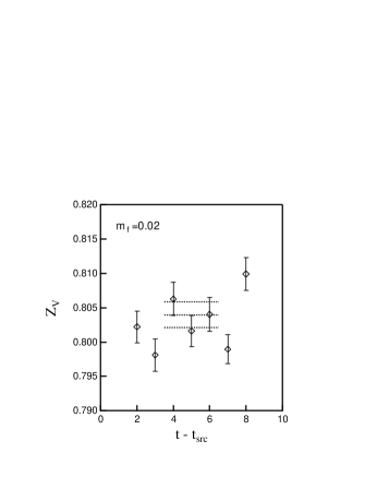
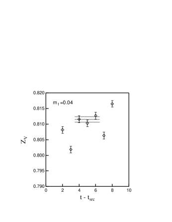
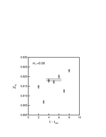
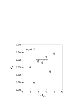
Figure 5: $Z_{{}_{V}}=1/g_{{}_{V}}^{\rm latt}$, DBW2 gauge action, $V\approx$ (2.4 fm)³, as a function of the current insertion time-slice. Note the very fine scale, same as in Figure 1. We use the three middle points, the spread of which is less than 0.5 %. The lines denote the central values and statistical errors from constant fits over them.

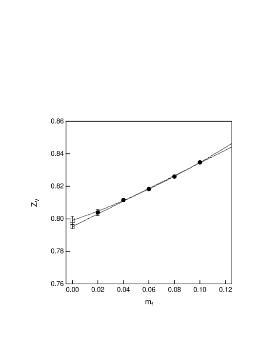
Figure 6: Same as Figure 2 except for the DBW2 gauge action, large volume.

First, we check whether $Z_{{}_{V}}=Z_{{}_{A}}$ is true even on this coarse lattice. The vector renormalization $1/g_{{}_{V}}^{\rm lattice}$ is plotted against the location of current insertions in Figure 5. The data are calculated on the larger spatial volume with the sequential quark propagator method. We take a weighted average of $1/g_{{}_{V}}^{\rm lattice}$ with the three middle points ($t-t_{\rm src}=4,5,6$) to evaluate the vector renormalization $Z_{{}_{V}}$. The dependence of $Z_{{}_{V}}$ on $m_{f}$ is shown in Figure 6 and given in Table 9. In general ${\cal V}_{\mu}=Z_{{}_{V}}V_{\mu}+{\cal O}(a^{2},m_{f}a^{2})$ and ${\cal A}_{\mu}=Z_{{}_{A}}A_{\mu}+{\cal O}(a^{2},m_{f}a^{2})$, where ${\cal V}_{\mu}$ and ${\cal A}_{\mu}$ denote the conserved vector currents. It is not so apparent in our data. A linear extrapolation yields $Z_{{}_{V}}=0.7952(13)$ at $m_{f}=0$, while a linear plus quadratic extrapolation gives the value 0.7991(25). The RBC collaboration obtained the renormalization factor of the axial-vector current $Z_{{}_{A}}$ nonperturbatively from a calculation of meson two-point correlation functions Blum:2000kn ; Aoki:2002vt . It was found $Z_{{}_{A}}=0.77759(45)$ in the massless limit Aoki:2002vt which is smaller than the value of $Z_{{}_{V}}$ obtained above by 2-3%. This discrepancy may be caused by an order ${\cal O}(a^{2})$ lattice artifact.

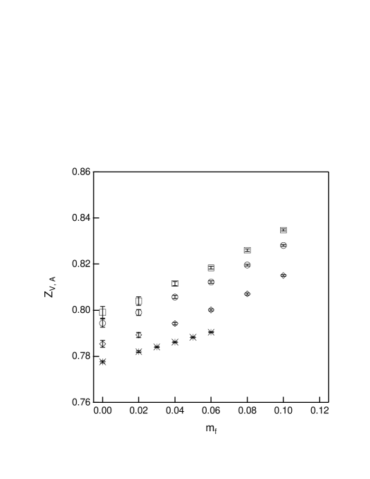
Figure 7: Determination of the vector current renormalization from $1/g_{{}_{V}}^{\rm latt}$ (squares), the electromagnetic current (circles), and the d-quark current (diamonds). The axial-vector current renormalization (bursts)Aoki:2002vt is shown for comparison. The different renormalization constants differ because of ${\cal O}(a^{2})$ lattice artifacts.

To explore this possibility further, we evaluate the renormalization factor of different vector currents. According to Sec.II, the conserved current ${\cal V}_{\mu}$ guarantees that nucleon matrix elements of $j_{\mu}^{em}$, ${\cal V}_{\mu}^{d}$ and ${\cal V}_{\mu}^{u}-{\cal V}_{\mu}^{d}$ should be identical. The local lattice currents $V_{\mu}^{f}$ are renormalized as ${\cal V}^{f}_{\mu}=Z_{{}_{V}}^{f}V^{f}_{\mu}+{\cal O}(a^{2})=Z_{{}_{V}}V^{f}_{\mu}+{\cal O}(a^{2})$ in the chiral limit. Figure 7 shows the values of $Z_{{}_{V}}^{f}$ as well as the value of $Z_{{}_{A}}$ from Aoki:2002vt . The difference among values of $Z_{{}_{V}}$ appears independent of $m_{f}$ within statistical errors, and the discrepancy between the smallest and the largest is comparable to that between $Z_{{}_{V}}$ and $Z_{{}_{A}}$ noted above. We also note that the discrepancy is larger at this lattice spacing, by roughly a factor $(1.922/1.3)^{2}$, than the corresponding one for the Wilson gauge action results discussed earlier. Of course, since the two gauge actions have different ${\cal O}(a^{2})$ errors, the comparison is only a crude one. We conclude that $Z_{{}_{V}}=Z_{{}_{A}}$ is satisfied up to small discretization errors of ${\cal O}(a^{2})$ on this coarse lattice.

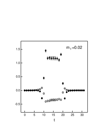
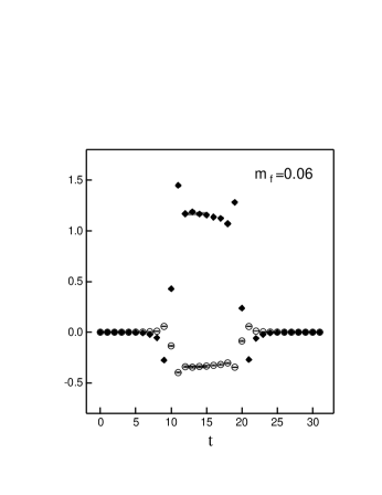
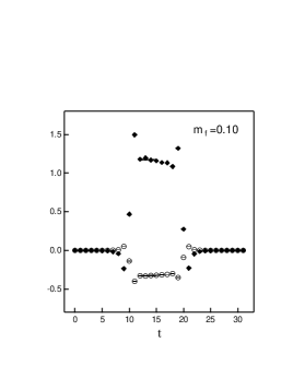
Figure 8: $\Delta u$ and $\Delta d$. Same as Figure 3, but for the DBW2 gauge action, sequential source, and $V=(2.4{\rm\,fm})^{3}$. The plateau is shifted towards the wall source because the point sink allows more excited state contamination.

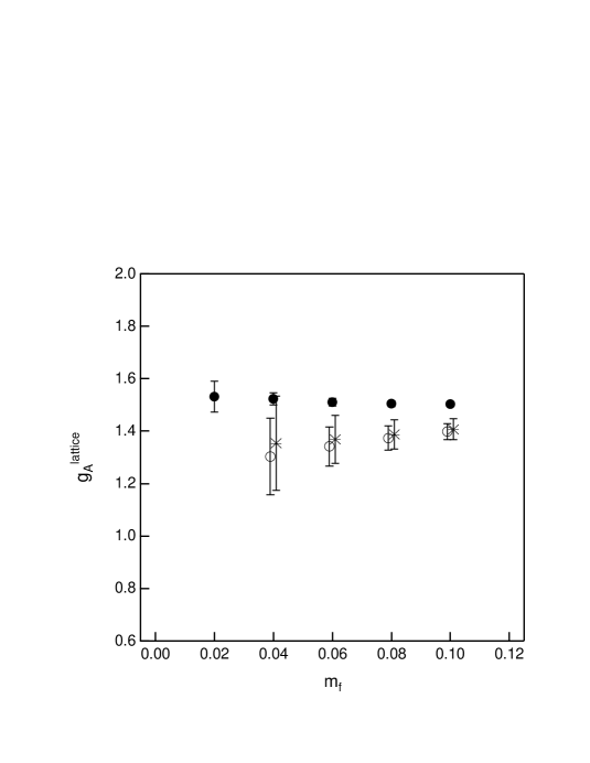
Figure 9: Dependence of the unrenormalized nucleon axial charge on quark mass and lattice volume. Results from the sequential source method (circles) and the wall source method (bursts) on the smaller lattice show good agreement. The sequential method provides somewhat smaller statistical errors than the wall method. The larger lattice results (solid circles), obtained with the sequential method, exhibit higher values than the smaller lattice ones over the entire range of quark mass studied.

In Figure 8 we plot unrenormalized spin-dependent densities $\Delta u$ and $\Delta d$, which are calculated with the sequential source propagator Martinelli:1989rr , against the location of the current insertion. In this calculation, the sequential source propagator was calculated with a box source and a point sink, so the resulting three-point function has no time reflection symmetry about the midpoint between $t_{\rm src}$ and $t_{\rm sink}$ because excited state contamination is worse for the nucleon propagating between the operator and the point sink. In Figure 8 the plateaus appear shifted toward the wall source, as expected. Next we evaluate the bare value of $g_{{}_{A}}^{\rm lattice}=\Delta u-\Delta d$ at each $m_{f}$, shown in Figure 9 for both lattice volumes and tabulated in Tables 8-9. $g_{{}_{A}}^{\rm lattice}$ evaluated on the smaller volume is clearly smaller for each value of $m_{f}$, and the difference increases as $m_{f}$ decreases. In contrast, $g_{{}_{V}}$ does not show much dependence on the volume.

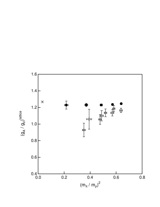
Figure 10: The physical ratio of nucleon charges. DBW2 gauge action results on two different physical volumes, $(2.4\rm\,fm)^{3}$ (solid circles) and $(1.2\rm\,fm)^{3}$ (open circles), reveal the existence of a significant finite volume effect. Wilson gauge action results (diamonds), $V\approx(1.6\,\rm fm)^{3}$, also appear to be affected by finite volume.

To compare to our previous DWF results with the Wilson gauge action, we plot the value of $(g_{{}_{A}}/g_{{}_{V}})^{\rm lattice}$ as a function of $(m_{\pi}/m_{\rho})^{2}$ in Figure 10. The smaller volume results using the DBW2 gauge action ($\beta=0.87$) are the same (within statistical errors) as our previous results using the Wilson gauge action ($\beta=6.0$) on a slightly larger volume. The large volume DBW2 results exhibit mild quark mass dependence while both smaller volume results show a marked decrease toward the chiral limit. We conclude that our previous DWF-Wilson-gauge-action results were significantly adversely affected by finite volume.

Finally, we extrapolate $g_{{}_{A}}^{\rm ren}$ to the chiral limit. For this purpose, we have two methods. One is to extrapolate the charge ratios $(g_{{}_{A}}/g_{{}_{V}})^{\rm lattice}$ to the chiral limit where the relation $Z_{{}_{V}}=Z_{{}_{A}}$ is valid. The second method is the conventional one utilized in all other calculations Fukugita:1995fh ; Liu:1994ab ; Gockeler:1996wg ; Gusken:1999as ; Dolgov:2002zm ; Capitani:1999zd ; Horsley:2000pz . The chiral extrapolation is performed on $g_{{}_{A}}^{\rm lattice}\times Z_{{}_{A}}$. Recall that the latter requires the value of $Z_{{}_{A}}$, whether nonperturbatively or perturbatively calculated, while the former does not. In the present case, we use the nonperturbative value of $Z_{{}_{A}}$ from Aoki:2002vt .

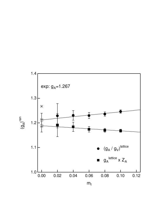
Figure 11: Two methods to obtain the physical nucleon axial charge, the ratio of axial-vector to vector charge (circles), and the lattice axial-vector charge times the axial-vector current renormalization factor $Z_{{}_{A}}$ in the chiral limit from Ref. Aoki:2002vt . They show slightly different quark mass dependence, but exptrapolate to consistent values. Each underestimates the experimental value (burst) by rougly five percent.

We plot $(g_{{}_{A}}/g_{{}_{V}})^{\rm lattice}$ and $Z_{{}_{A}}\times g_{{}_{A}}^{\rm lattice}$ together in Figure 11 and perform a simple linear extrapolation in each case. The two methods provide consistent results in the chiral limit: the ratio method gives $g_{{}_{A}}^{\rm ren}=1.212(27)$ while the conventional method gives $g_{{}_{A}}^{\rm ren}=1.188(25)$. In light of our earlier discussion, the systematic difference if there is one, is related to our choice of renormalization. A two percent error stemming from $Z_{{}_{V}}\neq Z_{{}_{A}}$ yields 0.024. This is also the difference in the central values just obtained. Thus, we quote

$$g_{{}_{A}}^{\rm ren}=1.212\pm 0.027({\rm stat})\pm 0.024({\rm norm})$$ (46)

which underestimates the experimental value of 1.267 by less than five percent. We have not attempted to estimate residual non-zero lattice spacing, finite volume, explicit chiral symmetry breaking, and quenching effects. The first three are probably small Blum:2000kn ; Aoki:2002vt ; AliKhan:2000iv . The only remaining error not under good control is the quenching one which does not appear to be large Gusken:1999as ; Dolgov:2002zm , in light of the relatively good agreement with experiment shown above. This view does not change unless significant non-analytic behavior, which we did not detect here, arises near the chiral limit.

We note Jaffe recently showed that in the chiral limit the nucleon axial charge is delocalized, and he argued this leads to a large reduction in $g_{{}_{A}}$ calculated in a finite volume surrounding the nucleon Jaffe:2001eb . Subsequently, Cohen showed that in a finite volume with periodic boundary conditions pertaining to lattice calculations, this phenomenon does not lead to a reduction in $g_{A}$ Cohen:2001bg . However, as emphasized in Cohen:2001bg , this does not preclude other large finite volume effects.

As mentioned above, this calculation of $g_{{}_{A}}$ is performed for relatively heavy quark masses; the quenching error at this unphysically large mass scale is probably small. However, one may worry that such a calculation does not capture relevant physics in the region where the quark mass is much lighter, and the so-called “pion cloud” surrounding the nucleon becomes important. Nevertheless the values of $g_{{}_{A}}^{\rm ren}$ at these heavier quark masses already lie just a few percent below the experimental value and show little dependence on the quark mass. This presents an important question concerning the role of the pion cloud: is it a few percent effect, as seems plausible from our first principles calculation, or is it larger, as estimated from phenomenological models Detmold:2002nf .

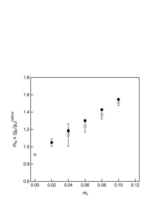
Figure 12: The lattice volume and quark mass dependences of the product $m_{{}_{N}}g_{{}_{A}}$. Renormalized. Closed (large volume) and open (small volume) circles. All agree within one standard deviation. No volume dependence is detected.

The dependence of the product $m_{{}_{N}}g_{{}_{A}}$ on the lattice volume is of interest (See Fig. 12). While the smaller volume results always lie below the larger volume ones, within one standard deviation they almost always agree. There is only one exception at $am_{f}=0.08$ in the bare lattice result. No volume dependence is detected. This is in clear contrast to the situation of the axial charge alone. Since the product is the one that appears in the Goldberger-Treiman relation, it would be interesting to see how its counterpart, the induced pseudo-scalar form factor, behaves at small momentum transfer.

IV Conclusions

In this paper we have studied the nucleon axial charge and the vector charge in quenched lattice QCD. To capture important aspects of the chiral symmetry of QCD, we used domain wall fermions to simulate the light quarks.

We first demonstrated that the lattice renormalization of the isovector vector and axial-vector currents satisfy $Z_{{}_{V}}=Z_{{}_{A}}$ to a high degree of precision, less than a percent at $a^{-1}\approx 2$ GeV and about two percent at $a^{-1}\approx 1.3$ GeV. This is achieved because in practice the DWF method preserves the chiral symmetry of QCD up to small corrections and hence maintains the relevant Ward-Takahashi identity. This holds if the underlying (quenched) gauge configuration is sufficiently smooth. Ensembles of such gauge configurations are obtained close to the continuum limit. For the single-plaquette Wilson gauge action $\beta=6.0$ ($a^{-1}\approx 2$ GeV) is good enough. For the DBW2 action the lattice spacing may be significantly larger while still maintaining good chiral symmetry ($a^{-1}\approx 1.3$ GeV).

Our first calculation of $g_{{}_{A}}$ with the Wilson gauge action was performed at $\beta=6.0$ on a $16^{3}\times 32$ lattice. The corresponding spatial volume $\sim(1.6{\rm fm})^{3}$ is similar to those used in previous lattice calculations. This volume is rather small in comparison with the experimentally measured proton charge radius. On this lattice we found all the relevant three-point functions are well behaved and that we can reliably extract the charges. The isovector vector current renormalization, $Z_{{}_{V}}$, determined from them agrees well with the corresponding axial current renormalization, $Z_{{}_{A}}$, independently obtained from the axial Ward-Takahashi identity. We found that both the axial charge, $g_{{}_{A}}^{\rm lattice}$, and its ratio to the vector charge, $(g_{{}_{A}}/g_{{}_{V}})^{\rm lattice}$, exhibit a very strong dependence on the quark mass. A simple linear extrapolation of $(g_{{}_{A}}/g_{{}_{V}})^{\rm lattice}$ to zero quark mass yielded a very small value, about 2/3 of the experimental one.

The second quenched calculation employed the DBW2 gauge action with $\beta=0.87$ set for a coarser lattice spacing, $a\approx 0.15$ fm. This allowed a larger physical volume while maintaining good chiral symmetry. To study pure finite volume effects, at fixed lattice spacing we calculated on lattices with sizes $16^{3}\times 32$ and $8^{3}\times 24$ ($\sim(1.2{\rm fm})^{3}$ and $\sim(2.4{\rm fm})^{3}$, respectively). A significant dependence on the volume is seen in both the axial charge $g_{{}_{A}}^{\rm lattice}$ and the charge ratio $(g_{{}_{A}}/g_{{}_{V}})^{\rm lattice}$, with the larger volume giving larger values. In contrast $g_{{}_{V}}$ does not show such dependence. The dependence on the quark mass is also different. In the larger volume the central values remain almost constant, while in the smaller volume they decrease noticeably with the quark mass. In the chiral limit the two differ by about 20% difference. The behavior of $g_{{}_{A}}$ on the smaller volume is quite consistent with that observed in the earlier calculation with the Wilson gauge action.

Our estimate of $(g_{{}_{A}}/g_{{}_{V}})^{\rm ren}$ at zero quark mass from the larger volume with DBW2 action is $1.212\pm 0.027({\rm stat})\pm 0.024({\rm norm})$. The systematic error is estimated from the two percent difference between $Z_{{}_{A}}$ and $Z_{{}_{V}}$ which are theoretically equivalent to ${\cal O}(a^{2})$, neglecting even smaller effects induced by explicit chiral symmetry breaking in DWF. It underestimates the experimental value of 1.2670(30) by less than five percent. This discrepancy is smaller than twice the theoretical error.

Thus dependence on the volume seems to be the largest among the known sources of systematic error for the first principles lattice calculation of $g_{{}_{A}}$. This suggests that close attention be paid to the finite volume effect in other lattice numerical studies of nucleon structure, in particular the moments of spin-polarized structure functions which are related to the axial charge.

It should be also noted that although the crucial relation $Z_{{}_{V}}=Z_{{}_{A}}$ is satisfied well in the second calculation, we detected small ${\cal O}(a^{2})$ differences among different determinations of $Z_{{}_{V}}$. Such differences were not detectable in the first set of simulations with the Wilson gauge action at $a\approx 0.10$ fm. Numerically this is at most a few percent effect, and does not affect the volume dependence.

As discussed at the end of section III, the present calculation of $g_{{}_{A}}$ was performed using relatively heavy quark masses (390 MeV $\leq m_{\pi}\leq$ 860 MeV) so that the systematic error arising from quenching may be small. However, one may worry that such a calculation does not capture the physics of the pion cloud surrounding the nucleon. In spite of this, the values of $g_{{}_{A}}^{\rm ren}$ at these unphysically heavy quark masses lie just below the experimental value and show little, if any, dependence on the quark mass. It is also interesting to note that the product $m_{{}_{N}}g_{{}_{A}}$ shows noticeably less volume dependence. Since this is the combination that appears in the Goldberger-Treiman relation, it would be interesting to see how its counterpart, the induced pseudo-scalar form factor, behaves at small but non-zero nucleon momentum.

Appendix A Current algebra and CVC hypothesis

Defining the charge ${\cal Q}_{{}_{V}}^{a}=i\int d^{3}xV_{0}^{a}(\vec{x},t)$ , the transformation for the quark fields in the isospin $SU(2)$ subgroup of the $SU(2)\times SU(2)$ chiral symmetry can be represented by

$$\left[{\cal Q}_{{}_{V}}^{a},\psi(x)\right] = -T^{a}\psi(x),$$ (47)

$$\left[{\cal Q}_{{}_{V}}^{a},{\bar{\psi}}(x)\right] = +{\bar{\psi}}(x)T^{a},$$ (48)

where $\psi=(u,d)^{T}$ and $V_{\mu}^{a}(x)={\bar{\psi}}(x)\gamma_{\mu}T^{a}\psi(x)$. One can easily find the axial current $A_{\mu}^{a}(x)={\bar{\psi}}(x)\gamma_{5}\gamma_{\mu}T^{a}\psi(x)$ and vector current $V_{\mu}^{a}$ transform under isospin symmetry as

$$\left[{\cal Q}_{{}_{V}}^{a},V_{\mu}^{b}(x)\right] = i\varepsilon_{abc}V_{\mu}^{c}(x)$$ (49)

$$\left[{\cal Q}_{{}_{V}}^{a},A_{\mu}^{b}(x)\right] = i\varepsilon_{abc}A_{\mu}^{c}(x).$$ (50)

According to the above $SU(2)$ current algebra, $A_{\mu}^{+}$ and $V_{\mu}^{+}$ can be expressed as

$$A_{\mu}^{\pm}(x) = {\bar{\psi}}(x)\gamma_{\mu}\gamma_{5}T^{\pm}\psi(x)=-[{\cal Q}_{{}_{V}}^{\pm},A_{\mu}^{3}(x)],$$ (51)

$$V_{\mu}^{\pm}(x) = {\bar{\psi}}(x)\gamma_{\mu}T^{\pm}\psi(x)=-[{\cal Q}_{{}_{V}}^{\pm},V_{\mu}^{3}(x)],$$ (52)

where $T^{\pm}=T_{1}\pm iT_{2}$. Hence, under the CVC hypothesis, one can find

$$\langle p|A_{\mu}^{+}|n\rangle = -\langle p|[{\cal Q}_{{}_{V}}^{+},A_{\mu}^{3}]|n\rangle$$ (53)

$$= -\langle p|{\cal Q}_{{}_{V}}^{+}A_{\mu}^{3}|n\rangle+\langle p|A_{\mu}^{3}{\cal Q}_{{}_{V}}^{+}|n\rangle$$

$$= \langle p|A_{\mu}^{3}|p\rangle-\langle n|A_{\mu}^{3}|n\rangle$$

$$= 2\langle p|A_{\mu}^{3}|p\rangle.$$

The third line follows from ${\cal Q}_{{}_{V}}^{+}|n\rangle=|p\rangle$ and $\langle p|{\cal Q}_{{}_{V}}^{+}=\langle n|$. A similar calculation for the vector case yields the relation, $\langle p|V_{\mu}^{+}|n\rangle=2\langle p|V_{\mu}^{3}|p\rangle$.

Table 1: Previous lattice calculations with Wilson or ${\cal O}(a)$ improved Wilson (clover) fermions. In general, $g_{{}_{A}}$ is significantly underestimated. Note that almost all volumes are small, most estimates use perturbative renormalization, and partially-unquenching did not increase the value of $g_{{}_{A}}$. The $\dagger$ symbol denote the continuum extrapolated value.

type	group	fermion	$L^{3}\times N_{t}$	$\beta$	volume	statistics	$m_{\pi}L$	$g_{{}_{A}}$	Ref.
quenched	KEK	Wilson	$16^{3}\times 20$	5.7	$({\rm 2.2fm})^{3}$	260	$\geq 5.9$	0.985(25)	Fukugita:1995fh
	Kentucky	Wilson	$16^{3}\times 24$	6.0	$({\rm 1.5fm})^{3}$	24	$\geq 5.8$	1.20(10)	Liu:1994ab
	DESY	Wilson	$16^{3}\times 32$	6.0	$({\rm 1.5fm})^{3}$	1000	$\geq 4.8$	1.074(90)	Gockeler:1996wg
	LHPC-SESAM	Wilson	$16^{3}\times 32$	6.0	$({\rm 1.5fm})^{3}$	200	$\geq 4.8$	1.129(98)	Dolgov:2002zm
	QCDSF	Wilson	$16^{3}\times 32$	6.0	$({\rm 1.5fm})^{3}$	O(500)		1.14(3)†	Capitani:1999zd
			$24^{3}\times 48$	6.2	$({\rm 1.6fm})^{3}$	O(300)
			$32^{3}\times 48$	6.4	$({\rm 1.6fm})^{3}$	O(100)
	QCDSF-UKQCD	Clover	$16^{3}\times 32$	6.0	$({\rm 1.5fm})^{3}$	O(500)		1.135(34)†	Horsley:2000pz
			$24^{3}\times 48$	6.2	$({\rm 1.6fm})^{3}$	O(300)
			$32^{3}\times 48$	6.4	$({\rm 1.6fm})^{3}$	O(100)
full($N_{f}=2$)	LHPC-SESAM	Wilson	$16^{3}\times 32$	5.5	$({\rm 1.7fm})^{3}$	100	$\geq 4.2$	0.914(106)	Dolgov:2002zm
	SESAM	Wilson	$16^{3}\times 32$	5.6	$({\rm 1.5fm})^{3}$	200	$\geq 4.5$	0.907(20)	Gusken:1999as

Table 2: Simulation parameters for each action and each volume studied in this work.

Gauge action	$\beta$	$L^{3}\times N_{t}$	$L_{s}$	$M_{5}$	volume
Wilson	6.0	$16^{3}\times 32$	16	1.8	$(1.6{\rm\,fm})^{3}$
DBW2	0.87	$16^{3}\times 32$	16	1.8	$(2.4{\rm\,fm})^{3}$
		$8^{3}\times 24$	16	1.8	$(1.2{\rm\,fm})^{3}$

Table 3: More parameters for each action and each volume.

Gauge action ($\beta$)	$L^{3}\times N_{t}$	quark mass values	statistics(type)	$m_{\pi}L$
Wilson (6.0)	$16^{3}\times 32$	0.02, 0.03, 0.04, 0.05	400 (Wall)	$\geq$4.3
DBW2 (0.87)	$16^{3}\times 32$	0.02, 0.04, 0.06, 0.08, 0.10	416 (Sequential)	$\geq$4.8
	$8^{3}\times 24$	0.04, 0.06, 0.08, 0.10	400 (Sequential)	$\geq$3.4
		0.04, 0.06, 0.08, 0.10	400 (Wall)

Table 4: The residual mass $m_{\rm res}$, hadron masses, inversre lattice spacing ($a^{-1}_{\rho}$, set by the $\rho$ meson mass) and the renormalization factor of the axial-vector current ($Z_{{}_{A}}$). The $\rho$ meson mass and the nucleon mass are given in the chiral limit in each case.

Gauge action ($\beta$)	$M_{5}$	$L_{s}$	$m_{\rm res}$	$m_{\rho}$	$m_{N}$	$a^{-1}_{\rho}$ (GeV)	$Z_{{}_{A}}$	Ref.
Wilson (6.0)	1.8	16	1.24 (5) $\times 10^{-3}$	0.404 (8)	0.566 (21)	1.922 (40)	0.7555 (3)	Blum:2000kn
DBW2 (0.87)	1.8	16	5.69 (26) $\times 10^{-4}$	0.589 (19)	0.780 (27)	1.31 (4)	0.77759 (45)	Aoki:2002vt

Table 5: Hadron masses computed using Wilson gauge action at $\beta=6.0$, $16^{3}\times 32$, $M_{5}=1.8$, $L_{s}=16$, from Ref.  Sasaki:2001nf .

$m_{f}$	$m_{\pi}$	$m_{\rho}$	$m_{N}$
0.02	0.2687 (24)	0.4530 (62)	0.645 (12)
0.03	0.3224 (21)	0.4814 (45)	0.716 (5)
0.04	0.3691 (19)	0.5126 (42)	0.754 (6)
0.05	0.4116 (18)	0.5395 (36)	0.805 (5)

Table 6: Results for the nucleon axial charge, $\Delta u$, $\Delta d$ and $Z_{{}_{V}}=1/g_{{}_{V}}^{\rm latt}$, Wilson gauge action, $\beta=6.0$, $16^{3}\times 32$, $M_{5}=1.8$, $L_{s}=16$, 400 configurations.

$m_{f}$	$(g_{{}_{A}})_{\rm latt}$	$(g_{{}_{A}})_{\rm ren}$	$(\Delta u)_{\rm ren}$	$(\Delta d)_{\rm ren}$	$Z_{{}_{V}}$
0.02	1.216 (106)	0.929 (82)	0.739 (82)	-0.189 (40)	0.7637 (23)
0.03	1.380 (76)	1.056 (59)	0.840 (54)	-0.215 (26)	0.7654 (17)
0.04	1.480 (59)	1.135 (46)	0.903 (40)	-0.232 (19)	0.7671 (13)
0.05	1.542 (47)	1.186 (37)	0.942 (32)	-0.243 (15)	0.7689 (11)

Table 7: Hadron masses computed using the DBW2 gauge action. All fits for $\rho$ meson have $\chi^{2}/N_{DF}<1.0$, and $<1.5$ for pion and nucleon.

$L^{3}\times N_{t}$	$m_{f}$	$m_{\pi}$	$m_{\rho}$	$m_{N}$
	0.04	0.4255 (38)	0.679 (16)	1.071 (13)
$8^{3}\times 24$	0.06	0.5094 (34)	0.729 (9)	1.127 (11)
	0.08	0.5865 (30)	0.776 (7)	1.205 (9)
	0.10	0.6567 (27)	0.823 (6)	1.292 (10)
	0.02	0.3015 (16)	0.647 (22)	0.854 (6)
	0.04	0.4146 (16)	0.681 (10)	0.963 (5)
$16^{3}\times 32$	0.06	0.5050 (16)	0.725 (6)	1.060 (4)
	0.08	0.5834 (15)	0.771 (5)	1.156 (4)
	0.10	0.6546 (14)	0.819 (4)	1.242 (4)

Table 8: Results for the nucleon axial charge, $\Delta u$, $\Delta d$ and $Z_{{}_{V}}=1/g_{{}_{V}}^{\rm latt}$, DBW2 gauge action, $\beta=0.87$, $8^{3}\times 24$, $M_{5}=1.8$, $L_{s}=16$, 400 configurations.

$m_{f}$	$(g_{{}_{A}})_{\rm latt}$	$(g_{{}_{A}})_{\rm ren}$	$(\Delta u)_{\rm ren}$	$(\Delta d)_{\rm ren}$	$Z_{{}_{V}}$
0.04	1.303 (146)	1.059 (120)	0.690 (99)	-0.369 (99)	0.8191(65)
0.06	1.342 (74)	1.099 (62)	0.817 (52)	-0.282 (45)	0.8242 (35)
0.08	1.373 (46)	1.136 (39)	0.876 (32)	-0.260 (25)	0.8317 (24)
0.10	1.398 (30)	1.165 (26)	0.902 (21)	-0.263 (15)	0.8403 (18)

Table 9: Results for the nucleon axial charge, $\Delta u$, $\Delta d$ and $Z_{{}_{V}}=1/g_{{}_{V}}^{\rm latt}$, DBW2 gauge action, $\beta=0.87$, $16^{3}\times 32$, $M_{5}=1.8$, $L_{s}=16$, 416 configurations.

$m_{f}$	$(g_{{}_{A}})_{\rm latt}$	$(g_{{}_{A}})_{\rm ren}$	$(\Delta u)_{\rm ren}$	$(\Delta d)_{\rm ren}$	$Z_{{}_{V}}$
0.02	1.531 (60)	1.229 (49)	0.945 (44)	-0.284 (27)	0.8040 (19)
0.04	1.523 (24)	1.230 (20)	0.946 (17)	-0.284 (10)	0.8115 (9)
0.06	1.510 (15)	1.230 (12)	0.953 (10)	-0.277 (6)	0.8184 (6)
0.08	1.505 (11)	1.236 (9)	0.963 (7)	-0.273 (4)	0.8260 (5)
0.10	1.503 (8)	1.246 (7)	0.975 (6)	-0.271 (3)	0.8347 (5)

Figure 1: $Z_{{}_{V}}=1/g_{{}_{V}}^{\rm latt}$, Wilson gauge action, as a function of the current insertion time-slice. Note the very fine scale. A good plateau for each quark mass is observed in the middle range between the source and sink. The lines denote central values and statistical errors from constant fits over the plateaus.

References

• (1) K. Hagiwara et al. [Particle Data Group Collaboration], Phys. Rev. D 66, 010001 (2002).
• (2) M. Fukugita, Y. Kuramashi, M. Okawa and A. Ukawa, Phys. Rev. Lett.  75, 2092 (1995) [arXiv:hep-lat/9501010].
• (3) K. F. Liu, S. J. Dong, T. Draper, J. M. Wu and W. Wilcox, Phys. Rev. D 49, 4755 (1994) [arXiv:hep-lat/9305025].
• (4) M. Göckeler, R. Horsley, E. M. Ilgenfritz, H. Perlt, P. Rakow, G. Schierholz and A. Schiller, Phys. Rev. D 53, 2317 (1996) [arXiv:hep-lat/9508004].
• (5) S. Güsken et al. [TXL Collaboration], Phys. Rev. D 59, 114502 (1999).
• (6) D. Dolgov et al. [LHPC collaboration], Phys. Rev. D 66, 034506 (2002) [arXiv:hep-lat/0201021].
• (7) S. Capitani et al., Nucl. Phys. Proc. Suppl.  79, 548 (1999) [arXiv:hep-ph/9905573].
• (8) R. Horsley [UKQCD Collaboration], Nucl. Phys. Proc. Suppl.  94, 307 (2001) [arXiv:hep-lat/0010059].
• (9) M. L. Goldberger and S. B. Treiman, Phys. Rev.  110, 1178 (1958).
• (10) M. Gell-Mann, R. J. Oakes and B. Renner, Phys. Rev.  175, 2195 (1968).
• (11) D. B. Kaplan, Phys. Lett. B 288, 342 (1992) [arXiv:hep-lat/9206013].
• (12) Y. Shamir, Nucl. Phys. B 406, 90 (1993) [arXiv:hep-lat/9303005].
• (13) R. Narayanan and H. Neuberger, Phys. Lett. B 302, 62 (1993) [arXiv:hep-lat/9212019].
• (14) V. Furman and Y. Shamir, Nucl. Phys. B 439, 54 (1995) [arXiv:hep-lat/9405004].
• (15) Y. Kikukawa, Nucl. Phys. B 584, 511 (2000) [arXiv:hep-lat/9912056].
• (16) P. Hernandez, K. Jansen and M. Luscher, Nucl. Phys. B 552, 363 (1999) [arXiv:hep-lat/9808010].
• (17) P. Hernandez, K. Jansen and M. Luscher, arXiv:hep-lat/0007015.
• (18) T. Blum et al., [RBC Collaboration], to appear in PRD, [arXiv:hep-lat/0007038].
• (19) A. Ali Khan et al. [CP-PACS Collaboration], Phys. Rev. D 63, 114504 (2001) [arXiv:hep-lat/0007014].
• (20) Y. Aoki et al., [RBC Collaboration], [arXiv:hep-lat/0211023].
• (21) T. Blum, Nucl. Phys. Proc. Suppl.  73, 167 (1999) [arXiv:hep-lat/9810017].
• (22) T. Blum et al., Phys. Rev. D 66, 014504 (2002) [arXiv:hep-lat/0102005].
• (23) T. Blum and S. Sasaki, arXiv:hep-lat/0002019.
• (24) T. Blum, S. Ohta and S. Sasaki, Nucl. Phys. Proc. Suppl.  94, 295 (2001) [arXiv:hep-lat/0011011].
• (25) N. Isgur and G. Karl, Phys. Rev. D 20, 1191 (1979).
• (26) A. Chodos, R. L. Jaffe, K. Johnson and C. B. Thorn, Phys. Rev. D 10, 2599 (1974).
• (27) T. Takaishi, Phys. Rev. D 54, 1050 (1996).
• (28) R. M. Woloshyn and K. F. Liu, Nucl. Phys. B 311, 527 (1989).
• (29) E. Jenkins and A. V. Manohar, Phys. Lett. B 259, 353 (1991).
• (30) G. Martinelli and C. T. Sachrajda, Nucl. Phys. B 316, 355 (1989).
• (31) C. W. Bernard, T. Draper, G. Hockney and A. Soni, in Proc. “Wuppertal 1985 Lattice Gauge Theory,” 199 (1985).
• (32) M. Kim and S. Kim, Phys. Rev. D 58, 074509 (1998) [arXiv:hep-lat/9608091].
• (33) S. Sasaki, T. Blum, S. Ohta and K. Orginos [RBC Collaboration], Nucl. Phys. Proc. Suppl.  106, 302 (2002) [arXiv:hep-lat/0110053].
• (34) S. Ohta [RBC Collaboration], arXiv:hep-lat/0210006.
• (35) L. l. Wu [RIKEN-BNL-CU collaboration], Nucl. Phys. Proc. Suppl.  83, 224 (2000) [arXiv:hep-lat/9909117].
• (36) R. L. Jaffe, Phys. Lett. B 529, 105 (2002) [arXiv:hep-ph/0108015].
• (37) T. D. Cohen, Phys. Lett. B 529, 50 (2002) [arXiv:hep-lat/0112014].
• (38) W. Detmold, W. Melnitchouk and A. W. Thomas, Phys. Rev. D 66, 054501 (2002) [arXiv:hep-lat/0206001].
• (39) S. Sasaki, T. Blum and S. Ohta, Phys. Rev. D 65, 074503 (2002) [arXiv:hep-lat/0102010].