A lattice calculation of vector meson couplings to the vector and tensor currents using chirally improved fermions

Abstract

We present a quenched lattice calculation of $f_{V}^{\perp}/f_{V}$, the coupling of vector mesons to the tensor current normalized by the vector meson decay constant. The chirally improved lattice Dirac operator, which allows us to reach small quark masses, is used. We put emphasis on analyzing the quark mass dependence of $f_{V}^{\perp}/f_{V}$ and find only a rather weak dependence. Our results at the $\rho$ and $\phi$ masses agree well with QCD sum rule calculations and those from previous lattice studies.

I Introduction

It is widely accepted that the rich spin structure of hard exclusive processes involving light vector $\rho,K^{*},\phi$ mesons provides a number of nontrivial possibilities to study the underlying short-distance dynamics. One example is given by vector meson electroproduction at large virtualities or large momentum transfers at HERA Crittenden (2002); Ciborowski (2002); Chekanov et al. (2003), HERMES Hartig (2000), and, in the future, COMPASS. In these cases the theoretical predictions for the production of longitudinally and transversely polarized mesons are very different Brodsky et al. (1994). Other examples are provided by exclusive semileptonic $B\to\rho\ell\nu_{\ell}$, rare radiative $B\to\rho\gamma$ or nonleptonic, $B\to\pi\rho$ etc. decays of $B$-mesons, which are attracting continuous interest as the prime source of information about the CKM mixing matrix; see, e.g., Ref. Battaglia et al. (2003) for an exposition of recent developments. In all cases, disentangling the longitudinally and transversely polarized (final) vector-meson states proves to be crucial since these cases often correspond to different underlying weak interaction physics. The theoretical description of such processes is developing rapidly and thus requires a more accurate and reliable determination of the relevant nonperturbative parameters.

From the vector meson side, the QCD description involves vector meson distribution amplitudes Efremov and Radyushkin (1980); Lepage and Brodsky (1980); Chernyak and Zhitnitsky (1984) which correspond to probability amplitudes for finding the quark and the antiquark in the meson with given momentum fractions and a small transverse separation. The distribution amplitudes for longitudinally polarized and transversely polarized vector mesons are different and their normalization (i.e. the integral over the momentum fractions) is given by the matrix elements of the vector and the tensor current

$$\left\langle 0\left|\bar{q}\gamma^{\mu}q\right|V(p;\lambda)\right\rangle = m_{V}\,f_{V}\,e_{\lambda}^{\mu}\;,$$ (1)

$$\left\langle 0\left|\bar{q}\sigma^{\alpha\beta}q\right|V(p;\lambda)\right\rangle = i\,f_{V}^{\perp}(\mu)\left(e_{\lambda}^{\alpha}p^{\beta}-e_{\lambda}^{\beta}p^{\alpha}\right)\;,$$ (2)

respectively. Here $V(p;\lambda)$ is a generic light vector meson with momentum $p$ and polarization vector $e_{\lambda}^{\alpha}$ such that $e_{\lambda}^{\alpha}p_{\alpha}=0$, $p^{2}=m_{V}^{2}$. Also $\sigma^{\alpha\beta}=\frac{i}{2}[\gamma^{\alpha},\gamma^{\beta}]$ and $q$ is the light quark field, $q=u,d,s\ldots\;$. In Eqs. (1), (2) we suppress the isospin structure, for brevity. The vector couplings $f_{V}$ are known from the experimental measurements in leptonic decays Hagiwara et al. (2002), while the tensor couplings $f_{V}^{\perp}$ have to be calculated using some nonperturbative approach. In particular, from QCD sum rules Ball and Braun (1996) one obtains

$$f_{\rho}^{\perp}\;=\;160\pm 10~{}\mbox{\rm MeV}\,,$$ (3)

($157\pm 5$ MeV in Ref. Bakulev and Mikhailov (2000)) and in the applications usually a very weak dependence on the quark mass of the ratios was assumed Chernyak and Zhitnitsky (1984); Ball and Braun (1998)

$$\frac{f_{\rho}^{\perp}}{f_{\rho}}\;\simeq\;\frac{f_{K^{*}}^{\perp}}{f_{K^{*}}}\;\simeq\;\frac{f_{\phi}^{\perp}}{f_{\phi}}\;\,.$$ (4)

(An earlier QCD sum rule determination of $f_{\rho}^{\perp}$ in Refs. Chernyak et al. (1983); Chernyak and Zhitnitsky (1984) suffers from a sign error, see Ref. Ball and Braun (1996).) At this place it is necessary to add that the couplings $f_{V}^{\perp}$, in contrast to $f_{V}$, are scale dependent. The corresponding anomalous dimension is equal to Shifman and Vysotsky (1981); Kumano and Miyama (1997); Hayashigaki et al. (1997)

$$\gamma^{T} = \frac{\alpha_{s}}{2\pi}C_{F}+\left(\frac{\alpha_{s}}{2\pi}\right)^{2}C_{F}\left(\frac{257}{36}C_{A}-\frac{19}{4}C_{F}-\frac{13}{18}N_{f}\right)$$ (5)

$$+\;{\cal O}(\alpha_{s}^{3})+...\;.$$

(The three-loop terms Gracey (2000), left out above simply for brevity, are included in our analysis.) The number in (3) is given for a low normalization point of $\mu=1$ GeV.

The error given in (3) does not include intrinsic uncertainties of the sum rule method itself which are difficult to quantify. Therefore, in view of the importance of this nonperturbative input for phenomenology, an independent confirmation of these numbers in a lattice calculation with controllable errors is extremely welcome. Earlier attempts were presented in Refs. Capitani et al. (1999); Becirevic et al. (2003) and the results agree well with the numbers from sum rules (there is also a current effort by the QCDSF Collaboration to determine $f_{\rho}^{\perp}$; the preliminary result also agrees with the sum rule result Göckeler et al. (2003)). These calculations were done with ${\cal O}(a)$ improved Wilson fermions. With this choice, however, one is restricted to relatively heavy pseudoscalars and the smallest pseudoscalar-mass to vector-mass ratio reached in Becirevic et al. (2003) is $m_{PS}/m_{V}$ = 0.56.

Here we present a new calculation of the matrix elements which is complementary to the first lattice results Becirevic et al. (2003). We use the recently developed Chirally Improved (CI) Dirac operator Gattringer (2001); Gattringer et al. (2001). It is based on the Ginsparg-Wilson relation Ginsparg and Wilson (1982) and has been shown Gattringer (2003); Gattringer et al. (2003a, b) to allow simulations with pseudoscalar-mass to vector-mass ratios down to $m_{PS}/m_{V}=0.28$ at relatively small cost.

In the results we present here we include lattice data down to $m_{PS}/m_{V}$ = 0.33 and thus push our calculation considerably closer to the chiral limit. Also at the heavy end we have additional data points such that our quark masses cover a range of $m_{PS}/m_{V}$ more than twice as large as the range in Becirevic et al. (2003). This allows us to check the weak quark-mass dependence of $f_{V}^{\perp}/f_{V}$ predicted by QCD sum rules. The data are compatible with a linear behavior in the quark mass, respectively in $m_{PS}^{2}$, and the slope is small. Only for our lightest quarks we find a deviation, which is, however, a finite size effect. Our final numbers agree well both with the QCD sum rule results and the lattice calculations in Refs. Capitani et al. (1999); Becirevic et al. (2003).

II Parameters of the calculation

We perform a quenched calculation with configurations from the Lüscher-Weisz gauge action Lüscher and Weisz (1985); Curci et al. (1983) and one step of HYP blocking Hasenfratz and Knechtli (2001). The final numbers we quote were computed on $16^{3}\times 32$ lattices at two different values of the gauge coupling, giving rise to lattice spacings of $a=0.15$ and $a=0.10$ fm Gattringer et al. (2002). For these lattices the parameters are listed in Table 1. In addition we performed a series of tests on smaller lattices ($12^{3}\times 24$, $8^{3}\times 24$) and at larger cutoff ($a=0.08$ fm). This serves to analyze the influence of finite volume and to study the scaling behavior.

We compute fermion propagators using the CI Dirac operator at 11 different bare quark mass values ranging from $am=0.01$ to $am=0.20$. These quark masses cover a range of $m_{PS}/m_{V}=0.33$ to $m_{PS}/m_{V}=0.92$. We do not encounter exceptional configurations and could work at even smaller quark masses. However, as we will show, decreasing the quark mass further, thus going closer to the chiral limit, is not sensible for a calculation of the matrix elements at the current physical volumes due to finite size effects.

In Gattringer (2003); Gattringer et al. (2003a, b) it is demonstrated that the CI operator is effectively ${\cal O}(a)$ improved. Furthermore the spectroscopy results presented there show only a very small variation in $a^{2}$ and thus are essentially free of scale dependence. However, improved operators are not yet available for the CI operator and thus for the matrix elements computed here one can expect only linear scaling in $a$ for our final results.

$\beta$	$a$ (fm) Gattringer et al. (2002)	$L$ (fm)	# confs.	$am_{q}$	$m_{PS}/m_{V}$ Gattringer et al. (2003a)
7.90	0.15	2.4	100	0.02 - 0.20	0.38 - 0.85
8.35	0.10	1.6	100	0.01 - 0.20	0.33 - 0.92

Table 1: Parameters for our large lattices ($16^{3}\times 32$).

The renormalization constants necessary for our observables were calculated according to the method presented in Martinelli et al. (1995); Göckeler et al. (1999). The procedure is patterned after the definition used in the continuum. In a fixed gauge (we use the Landau gauge) the numerically evaluated amputated Green’s functions are compared to their tree level counterparts and the renormalization constants are read off. The resulting numbers are in the so-called RI-MOM scheme and are converted to $\overline{\mbox{MS}}$ using the perturbative matching coefficients. For the vector and tensor renormalization constants, however, these matching constants are 1 up to NLO in perturbation theory. A detailed analysis of renormalization for the CI operator will be presented in Gattringer et al. (2003c) and here we only quote the numbers we need.

The renormalization constants were evaluated for the same set of quark masses that was also used in the calculation of the matrix elements. When plotted as a function of the quark mass, the data are found to follow a straight line very well and the chiral extrapolation is straightforward. This procedure was repeated for several values of the 4-momentum $p$. Following Becirevic et al. (2003) we base our calculation on the numbers extracted at the cutoff, i.e. at $p^{2}=a^{-2}$. To get the numbers at exactly $a^{-2}$ we linearly interpolated the chirally extrapolated values of $Z_{V},Z_{T}$ between the two momenta with $p^{2}$ just above and below $a^{-2}$. The resulting numbers for $Z_{T}$ were then evolved to our target scale of $\mu$ = 2 GeV using the renormalization group equation. $Z_{V}$ remains constant as a function of $\mu$ (no anomalous dimension) and we used the value at $\mu^{2}=a^{-2}$. Our numbers for $Z_{V}$ and $Z_{T}$ are listed in Table 2.

$\beta$	$Z_{V}(a^{-1})$	$Z_{T}(a^{-1})$	$Z_{T}$(2 GeV)	$Z_{T}/Z_{V}$(2GeV)
7.90	0.9346(7)	1.0598(10)	1.0247(10)	1.0964(19)
8.35	0.9780(14)	1.0542(19)	1.0532(20)	1.0768(37)

Table 2: Results for the renormalization constants. The numbers in parenthesis give the scale $\mu$. It is either the cutoff ($\mu=a^{-1}$) or $\mu=$ 2 GeV.

III Extraction of the raw data

If we only consider the vector-meson contribution to the vector-vector (VV) and vector-tensor (VT) correlators and contract two of the Lorentz indices, we arrive at the following expressions:

$$g_{\mu\nu}\,\left\langle 0\left|\bar{q}\gamma^{\mu}q\right|V(p;\lambda)\right\rangle\left\langle V(p;\lambda)\left|\bar{q}\gamma^{\nu}q\right|0\right\rangle=$$

$$m_{V}^{2}\,f_{V}^{2}\,\left(e_{\lambda}^{\mu}e_{\lambda}^{\nu*}\,g_{\mu\nu}\right)\;,$$ (6)

$$g_{\mu\nu}\,\left\langle 0\left|\bar{q}\gamma^{\mu}q\right|V(p;\lambda)\right\rangle\left\langle V(p;\lambda)\left|\bar{q}\sigma^{\alpha\nu}q\right|0\right\rangle=$$

$$i\,m_{V}\,f_{V}\,f_{V}^{\perp}(\mu)\,p^{\alpha}\,\left(e_{\lambda}^{\mu}e_{\lambda}^{\nu*}\,g_{\mu\nu}\right)\;,$$ (7)

where $e_{\lambda}^{\mu}e_{\lambda}^{\nu*}g_{\mu\nu}=-3$. Taking the ratio of these (vector-tensor/vector-vector), we have

$$R^{\alpha}=\frac{ip^{\alpha}f_{V}^{\perp}(\mu)}{m_{V}f_{V}}\;,$$ (8)

with one remaining Lorentz index from the tensor current. It is this ratio we wish to extract in our lattice calculation.

For the non-zero-momentum correlators, however, there is an additional complication, which arises because the quark sources are smeared in the spatial directions. Since the smearing is not performed in the time direction as well, Lorentz symmetry is lost, affecting the $e_{\lambda}^{\nu}p_{\nu}=0$ condition (checking this relation explicitly with the different Lorentz components of the $\vec{p}\not=0$, VT correlators, we find the discrepancy to be small, but significant). More explicitly, we have for the VT correlator

$$\left\langle 0\left|(U\bar{q})\gamma^{\mu}(Uq)\right|V(p;\lambda)\right\rangle\left\langle V(p;\lambda)\left|\bar{q}\sigma^{\alpha\nu}q\right|0\right\rangle=$$

$$i\,m_{V}\,f_{V}\,f_{V}^{\perp}(\mu)\,Z_{U}(p)\,e_{\lambda}^{\mu}\left(e_{\lambda}^{\nu*}p^{\alpha}-e_{\lambda}^{\alpha*}p^{\nu}\right)\;,$$ (9)

where $U$ represents the smearing operator and $Z_{U}(p)$ is the corresponding factor for the amplitude. For the $\alpha=j$ case, we may no longer sum over all of the Lorentz indices, $\mu=\nu$, and still expect the second term to vanish. We may, however, consider only the contributions where $\mu=\nu=k\not=j$ and $p^{k}=0$. Then, using only the $\nu=k$, $p^{k}=0$ contributions for the VV correlator as well, we have the appropriate cancellations in the ratio $R^{j}(\vec{p})$. This finite-momentum ratio yields much larger statistical errors than the zero-momentum ratio, $R^{0}(0)$, and we pursue this approach only as a consistency check.

We note here that the smearing has no effect upon the zero-momentum results since these have contributions only from the spatial components of the vector-current source and the smearing amplitude, $Z_{U}(p)$, is the same for all spatial directions at $\vec{p}=0$.

The Euclidean lattice formulation provides a natural selection of the desired vector-meson contribution to our correlators; we simply need to ensure that our two currents are separated by a large enough distance in the imaginary time direction. The vector-vector correlator, which corresponds to Eq. (6), thus reads

$$C^{VV}(\vec{p}\,;t)\;=\;\sum_{\vec{x}}\;e^{i\vec{p}\cdot\vec{x}}\;\left\langle\left(\bar{\psi}\gamma_{k}\psi\right)_{0,0}\left(\bar{\psi}\gamma_{k}\psi\right)_{\vec{x},t}\right\rangle\;.$$ (10)

We project to definite momentum $\vec{p}$, using the necessary phase factor, and sum over the relevant, spatial Lorentz indices, $k$ ($p_{k}=0$). For the tensor current we have to distinguish two different cases: When the open tensor index is time ($=4$) we consider the temporal correlator $C^{VT}_{4}$ defined as ($k$ is summed)

$$C^{VT}_{4}(\vec{p}\,;t)\;=\;i\sum_{\vec{x}}\;e^{i\vec{p}\cdot\vec{x}}\;\left\langle\left(\bar{\psi}\gamma_{k}\psi\right)_{0,0}\left(\bar{\psi}\sigma_{k4}\psi\right)_{\vec{x},t}\right\rangle\;.$$ (11)

For open spatial tensor indices $j=1,2,3$ we study the spatial correlator $C^{VT}_{j}$ defined as

$$C^{VT}_{j}(\vec{p}\,;t)\;=\;\sum_{\vec{x}}\;e^{i\vec{p}\cdot\vec{x}}\;\left\langle\left(\bar{\psi}\gamma_{k}\psi\right)_{0,0}\left(\bar{\psi}\sigma_{kj}\psi\right)_{\vec{x},t}\right\rangle\;,$$ (12)

where $p_{j}\not=0$ and the sum over $k$ is restricted to the two values different from $j$, such that $p_{k}=0$. The temporal and spatial correlators $C^{VT}_{4}$ and $C^{VT}_{j}$ differ in two respects: Firstly, the spatial correlator is non-vanishing only for non-zero momenta, while the temporal correlator gives a contribution also at zero momentum. Secondly, the spatial and temporal correlators differ by their time reversal symmetries. In particular one finds:

$$C^{VV}(\vec{p}\,;t) = A^{VV}(\vec{p}\,)\left(e^{-E_{V}(\vec{p}\,)t}+e^{E_{V}(\vec{p}\,)(t-T)}\right)+...\;,$$

$$C^{VT}_{4}(\vec{p}\,;t) = A^{VT}_{4}(\vec{p}\,)\left(e^{-E_{V}(\vec{p}\,)t}-e^{E_{V}(\vec{p}\,)(t-T)}\right)+...\;,$$

$$C^{VT}_{j}(\vec{p}\,;t) = A^{VT}_{j}(\vec{p}\,)\left(e^{-E_{V}(\vec{p}\,)t}+e^{E_{V}(\vec{p}\,)(t-T)}\right)+...\;.$$

The dots indicate corrections due to excited states which play a role only at small time separations but become suppressed exponentially for larger values of $t$.

Let us have a first look at our data for $C^{VV}$ and $C^{VT}$, separately. This serves to check how well the expected behavior of Eqs. (LABEL:larget) is seen and how serious the effects of excited states are. For this test and also for the extraction of the data we fold all correlators about $T/2$ according to their time-reversal symmetries and average them appropriately. In the plots we thus show only the folded and averaged correlator in the range $t=0\;...\;T/2$.

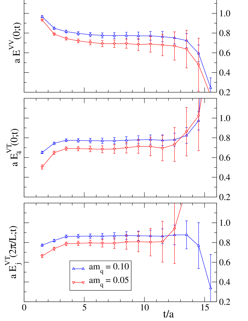
Figure 1: Effective masses for the vector-vector (top plot), temporal vector-tensor (middle plot) and spatial vector-tensor (bottom plot) correlators. The effective mass for the spatial vector-tensor correlator is shown for momentum $\vec{p}\,^{2}=(2\pi)^{2}/L^{2}$, while the other two effective masses are for zero momentum. The data shown here are for the $16^{3}\times 32$ lattices with $a=0.15$ fm and two values of the bare quark mass, $am_{q}=0.05,0.10.$

In Fig. 1 we show effective mass plots, i.e. $\ln[C(t)/C(t+1)]$, for our folded correlators defined in Eqs. (10) – (12). The effective mass $E^{VV}$ for the vector-vector correlator (top plot) and the effective mass $E^{VT}_{4}$ for the temporal vector-tensor correlator (middle plot) are shown for zero momentum, while the effective mass $E^{VT}_{j}$ for the spatial vector-tensor correlator (bottom plot) is shown for momentum $\vec{p}\,^{2}=(2\pi)^{2}/L^{2}$. The data for the figure are from the $16^{3}\times 32$ lattices with $a=0.15$ fm and two values of the bare quark mass, $am_{q}=0.05,0.10$. The spatial correlator has been averaged over all three components $j=1,2,3$. However, the scatter of the results for the individual components $j$ is small.

Both vector-tensor correlators show plateaus between $t/a=4$ and $t/a=12$ and the vector-vector correlator for $t/a=6\;...\;12$. For smaller time separations it is obvious that contributions from excited states are important. For $t/a$ larger than 12 we observe two effects: Firstly, an increase of the error bars which is simply an effect of the reduced signal to noise ratio for longer propagation in $t$ and, secondly, a systematic deviation from the plateau due to the sinh / cosh behavior of the correlators. For all quark masses we looked at we were able to identify stable plateaus. When comparing our different results for the vector meson energy $E_{V}(\vec{p}\,)$ which determines the time behavior of all three correlators [see Eq. (LABEL:larget)] we found that the values of $E_{V}(\vec{p}\,)$ agreed well for the different operators. Note that the spatial vector-tensor correlator shown in the bottom plot of Fig. 1 is for nonzero momentum and thus its plateau is slightly higher than for the other two correlators.

Once the amplitudes are known we can form the temporal and spatial ratios $R_{4}$ and $R_{j}$ defined as

$$R_{4}(\vec{p}\,) = A^{VT}_{4}(\vec{p}\,)/A^{VV}(\vec{p}\,)\;,$$

$$R_{j}(\vec{p}\,) = A^{VT}_{j}(\vec{p}\,)/A^{VV}(\vec{p}\,)\;.$$ (14)

We have already remarked that $R_{4}$ is non-vanishing also at zero momentum, while $R_{j}$ gives a contribution only for non-zero momenta. Since the quality of lattice correlators generally is decreasing with increasing momenta we evaluate $R_{4}$ at zero momentum and $R_{j}$ at the smallest possible momentum, i.e., $\vec{p}\,^{2}=(2\pi)^{2}/L^{2}$. The ratios $f_{V}^{\perp}/f_{V}$ are then obtained from

$$R_{4}(0)=\frac{f_{V}^{\perp}}{f_{V}}\;\;,\;\;R_{j}(\vec{p}\,)=\frac{p_{j}\;f_{V}^{\perp}}{m_{V}\;f_{V}}\;.$$ (15)

For the vector mass $m_{V}$ in the second equation we may use the value obtained from our fits to the same correlators; i.e., $m_{V}=\sqrt{E_{V}^{\,2}(\vec{p}\,)-\vec{p}^{\,2}}$. Note that here $f_{V}$ and $f_{V}^{\perp}$ are bare lattice quantities which need to be renormalized.

IV Results

In order to extract the appropriate values for the amplitudes, $A^{VV}$ and $A^{VT}_{\nu}$, from the two separate correlators, we construct a $\chi^{2}$ measure of the form

$$\chi^{2} = \sum_{I,J}\sum_{t^{I},t^{J}}\left[C^{I}(\vec{p}\,;t^{I})-C_{exp}^{I}(\vec{p}\,;t^{I})\right]$$ (16)

$$\;\times\;S_{I,J}^{-1}(t^{I},t^{J})\left[C^{J}(\vec{p}\,;t^{J})-C_{exp}^{J}(\vec{p}\,;t^{J})\right]$$

$$= F\left(A^{VV}(\vec{p}\,),A^{VT}_{\alpha}(\vec{p}\,),E_{V}(\vec{p}\,)\right)\;,$$

where the “expected” values, $C_{exp}^{I}(\vec{p}\,;t)$, are given by the appropriate expressions in Eqs. (LABEL:larget) and $S^{-1}$ is the inverse of the covariance matrix. We extract the three parameters by minimizing the above function, taking care to use large enough minimum $t^{I}$ values, thereby avoiding excited-state contributions. See Table 3 for the results of the zero-momentum fits.

Since we are interested in the ratios of the resulting amplitudes, we repeat these fits within a single-elimination jackknife routine, providing the errors for $f_{V}^{\perp}/f_{V}$ (see the final column of Table 3).

$a$ (fm)	$am_{q}$	$t^{VV}$	$t^{VT}$	$\chi^{2}$/d.o.f.	$R_{4}(0)$
0.15	0.02	$8-12$	$4-12$	10/11	0.678(36)
′′	0.03	$8-13$	$4-13$	11/13	0.680(24)
′′	0.04	$8-15$	$4-14$	14/16	0.688(18)
′′	0.05	$8-16$	$4-15$	18/18	0.696(14)
′′	0.06	$8-16$	$4-15$	18/18	0.707(10)
′′	0.08	$8-16$	$4-15$	17/18	0.725(7)
′′	0.10	$8-16$	$4-15$	16/18	0.740(5)
0.10	0.04	$9-16$	$6-15$	21/15	0.716(9)
′′	0.05	$9-16$	$6-15$	23/15	0.722(7)
′′	0.06	$9-16$	$6-15$	25/15	0.729(6)
′′	0.08	$9-16$	$6-15$	29/15	0.744(4)

Table 3: Selected results (those used for the quark mass extrapolation) of the three-parameter fits for the zero-momentum correlators.

Figure 2: Ratio of vector meson couplings (at the lattice scale, $\mu=1/a$) as a function of $r_{0}^{2}m_{PS}^{2}$ for the two lattice spacings. The dashed vertical lines denote the $r_{0}^{2}m_{\pi}^{2}$ and $r_{0}^{2}m_{s\bar{s}}^{2}$ ($m_{s\bar{s}}^{2}=2m_{K}^{2}-m_{\pi}^{2}$) physical values. The bursts denote the mass interpolations at $m_{s\bar{s}}^{2}$ and extrapolations to $m_{\pi}^{2}$.

Figure 2 displays the ratios of the vector meson couplings as a function of the dimensionless quantity, $r_{0}^{2}m_{PS}^{2}$. For a wide range of quark masses the data display only a slight curvature and are quite compatible with a linear behavior. Only for the smallest quark masses do the data move upwards. Simulations on smaller physical volumes ($8^{3}\times 24$ and $12^{3}\times 24$) at a fixed lattice spacing ($a$ = 0.15 fm) suggest that the upward trend of the ratio at small quark masses is a finite-size effect. This interpretation is supported by the observation that also in spectroscopy calculations of nucleons and their excitations the finite size effects set in at the same values of the quark mass Gattringer (2003); Gattringer et al. (2003a, b). In order to avoid including such effects, we perform the (fully correlated) extrapolation to light quark mass without some of the lightest bare quark masses.

	$a=0.15$ fm	$a=0.10$ fm
$\left(\frac{f_{\phi}^{\perp}}{f_{\phi}}\right)_{\overline{\rm MS}}$(2 GeV)	0.801(7)	0.780(8)
$\left(\frac{f_{\rho}^{\perp}}{f_{\rho}}\right)_{\overline{\rm MS}}$(2 GeV)	0.720(25)	0.742(14)

Table 4: $f_{V}^{\perp}/f_{V}$ values in the $\overline{\rm MS}$ scheme at $\mu=2$ GeV as determined from the lattice ratio $R_{4}(0)$.

This is necessary only for our fine lattices ($\beta=8.35$), where the three smallest quark masses give rise to pseudoscalars with $m_{PS}L<4$. As can be seen in the plot, it is exactly these three data points which show finite-size effects and we therefore exclude them from the chiral extrapolation. For our larger lattices ($\beta=7.90$), we always have $m_{PS}L>4$; no finite-size effects are visible and all data points are included in the fit. On the heavy end, all masses with $r_{0}^{2}m_{PS}^{2}>5$ are also excluded from the extrapolation. To obtain the data at the strange quark mass we interpolate the neighboring data linearly.

In Table 4 we present our final results for the ratios of the couplings, matched to the $\overline{\rm MS}$ scheme and evolved to the scale of 2 GeV. These results are obtained from the zero-momentum correlator ratios, $R_{4}(0)\times Z_{T}/Z_{V}(2\,{\rm GeV})$.

Figure 3: Similar plot to that of Fig. 2, this time for the finite-momentum ratio $m_{V}R_{j}(\vec{p}\,)/p_{j}$, where $|\vec{p}\,|=p_{j}=2\pi/L$. The symbols have the same meaning as before.

Since we include no improvement in our current operators, we may expect a lattice spacing dependence of ${\cal O}(a)$. However, since we only have results for two values of the lattice spacing, a continuum extrapolation becomes problematic.

	$a=0.15$ fm	$a=0.10$ fm
$\left(\frac{f_{\phi}^{\perp}}{f_{\phi}}\right)_{\overline{\rm MS}}$(2 GeV)	0.805(15)	0.746(24)
$\left(\frac{f_{\rho}^{\perp}}{f_{\rho}}\right)_{\overline{\rm MS}}$(2 GeV)	0.740(39)	0.700(38)

Table 5: $f_{V}^{\perp}/f_{V}$ values in the $\overline{\rm MS}$ scheme at $\mu=2$ GeV as determined from the lattice ratio $R_{j}(2\pi/L)$.

We do note that the two results for the $\rho$ meson are consistent with each other and they are also in agreement with the results of other lattice calculations Capitani et al. (1999); Becirevic et al. (2003): $0.72(2)(^{+2}_{-0})$ in Ref. Becirevic et al. (2003). The trend of the $\phi$ results suggests a continuum value below our $\beta=8.35$ result of 0.78, in rough agreement with the 0.76(1) result of Ref. Becirevic et al. (2003).

If we normalize using the experimental value of $f_{\rho^{\pm}}^{\,\rm exp.}\approx 208$ MeV Hagiwara et al. (2002); Becirevic et al. (2003), we find good agreement with the QCD sum rule result Ball and Braun (1996, 1998); Bakulev and Mikhailov (2000): $f_{\rho}^{\perp}/f_{\rho^{\pm}}^{\,\rm exp.}=0.74(3)$. Such comparisons, however, are difficult to assess due to the different systematics in the two approaches (e.g., our lattice calculation is quenched).

The results for the finite-momentum correlator ratio, $R_{j}(\vec{p}\,)$, are shown in Fig. 3. The quark-mass interpolations and extrapolations are performed just as before for the zero-momentum ratios.

Table 5 displays the renormalized coupling ratios obtained from the non-zero-momentum correlator ratios. The errors are significantly larger for these than those for the zero-momentum results. However, the results of this consistency check are compatible with those from the zero-momentum ratios ($<1.5\sigma$ even for the jackknifed difference at and below the strange-quark mass).

Let us briefly summarize our findings. We calculate $f_{V}^{\perp}/f_{V}$ going considerably closer to the chiral limit (at least on our larger lattices where the results do not display significant finite-volume effects) than previous calculations. This allows us to monitor the mass dependence of this ratio of couplings over a much larger mass range. We find the quark mass dependence to be relatively weak, as in QCD sum rule calculations. The values we obtain agree well with the extrapolated values of other lattice calculations at larger quark masses. We include a consistency check using spatial tensor correlators at finite momentum and find compatible results. Our final numbers are $f_{\rho}^{\perp}/f_{\rho}=0.720(25),\,0.742(14)$ and $f_{\phi}^{\perp}/f_{\phi}=0.801(7),\,0.780(8)$ at $a=0.15,\,0.10$ fm, respectively.