Numerical determination of monopole entropy
in pure SU(2) QCD

Abstract

We study numerically the length distributions of the infrared monopole clusters in pure SU(2) QCD. These distributions are Gaussian for all studied blocking steps of monopoles, lattice volumes and lattice coupling constant. We also investigate the monopole action for the infrared monopole clusters. The knowledge of both the length distribution and the monopole action allows us to determine the effective entropy of the monopole currents. The entropy is a descending function of blocking scale, indicating that the effective degrees of freedom of the extended monopoles are getting smaller as the blocking scale increases.

I Introduction

The dual superconductor picture DualSuperconductor of the QCD vacuum is one of the most promising approaches to the problem of color confinement. This picture is based on the existence of Abelian monopoles in the vacuum of QCD. The monopoles are identified with the help of the so-called Abelian projection method AbelianProjections , which is based on the partial gauge fixing of the SU(N) gauge symmetry up to an Abelian subgroup. The monopoles naturally appear in the Abelian projection due to compactness of the residual Abelian group.

There are various numerical indications that the monopoles are responsible for the confinement of quarks (for a review, see Ref. Reviews ). One of the most important observations is the monopole condensation in the low temperature (confinement) phase shiba:condensation ; MonopoleCondensation . According to the dual superconductor mechanism the monopole condensation give rise to the formation of the chromoelectric string which confines the fundamental color sources. This expectation is confirmed by the fact that the non–zero tension of the chromoelectric string is dominated by the Abelian monopole contributions AbelianDominance ; shiba:string ; koma:string .

In the numerical simulations one observes that the trajectories of the Abelian monopoles form clusters, which can be divided by two ensembles: finite-sized clusters and one large percolating cluster ivanenko ; ref:kitahara ; ref:hart . The percolating cluster (or, infrared cluster) occupies the whole lattice while the sizes of the other clusters have an ultraviolet nature. The existence of the IR cluster is related to the monopole condensation ivanenko . This is understandable on an intuitive level, since generally the condensation is a microscopic effect reflecting itself in a zero–momentum component of the condensed field. The importance of the IR cluster for the confinement of quarks was also stressed in numerical calculations ref:kitahara : the tension of the confining string gets a dominant contribution from the monopoles belonging to the IR cluster, while the contribution of the UV clusters to the string tension is negligible. In the deconfinement phase the IR cluster disappears ivanenko ; ref:kitahara , as expected.

In this paper we mostly concentrate on the numerical investigation of the properties of the infrared monopole cluster. The length distributions and other properties of the UV and IR clusters were studied previously in Refs. ref:zakharov:clusters ; ref:hart ; ref:kitahara ; ref:boyko ; zakharov:recent . In this publication we are going to investigate thoroughly the properties of the length distributions of the monopole clusters for various lattice volumes and sizes of the extended monopoles.

The plan of the paper is the following. In Section II we describe the model and provide the details of numerical simulations. Section III is devoted to the investigation of the Abelian monopole action obtained by the inverse Monte-Carlo method. The distribution of the cluster length in the infrared clusters is studied in Section IV. The knowledge of the monopole action and cluster distribution allows us, for the first time, to calculate the entropy of the lattice monopoles of various sizes. Our conclusions are presented in the last Section.

II Model and simulation details

We study the pure SU(2) gluodynamics with the lattice Wilson action, $S(U)=-\frac{\beta}{2}{\mathrm{Tr}}U_{P}$, where $\beta$ is the coupling constant and $U_{P}$ is the SU(2) plaquette constructed from the link fields. All our results are obtained in the Maximal Abelian (MA) gauge kronfeld which is defined by the maximization of the lattice functional

$$R=\sum_{s,\hat{\mu}}{\rm Tr}\Big{(}\sigma_{3}\widetilde{U}(s,\mu)\sigma_{3}\widetilde{U}^{\dagger}(s,\mu)\Big{)}\,,$$ (1)

with respect to the gauge transformations $U(s,\mu)\to\widetilde{U}(s,\mu)=\Omega(s)U(s,\mu)\Omega^{\dagger}(s+\hat{\mu})$. The local condition of maximization can be written in the continuum limit as the differential equation $(\partial_{\mu}+igA_{\mu}^{3})(A_{\mu}^{1}-iA_{\mu}^{2})=0$. Both this condition and the functional (1) are invariant under residual U(1) gauge transformations, $\Omega^{\mathrm{Abel}}(\omega)={\mathrm{diag}(e^{i\omega(s)},e^{-i\omega(s)})}$.

The next step is Abelian projection of non–Abelian link variables to the Abelian ones after the gauge fixing is done. An Abelian gauge field is extracted from the $SU(2)$ link variables as follows:

$$\widetilde{U}(s,\mu)=\left(\begin{array}[]{cc}(1-|c(s,\mu)|^{2})^{1/2}&-c^{*}(s,\mu)\\ c(s,\mu)&(1-|c(s,\mu)|^{2})^{1/2}\end{array}\right)\left(\begin{array}[]{cc}u(s,\mu)&0\\ 0&u^{*}(s,\mu)\end{array}\right),$$ (6)

where $u(s,\mu)=\exp(i\theta(s,\mu))$ represents the Abelian link field and $c(s,\mu)$ corresponds to charged matter fields.

The Abelian field strength $\theta_{\mu\nu}(s)\in(-4\pi,4\pi)$ is defined on the lattice plaquettes by a link angle $\theta(s,\mu)\in[-\pi,\pi)$ as $\theta_{\mu\nu}(s)=\theta(s,\mu)+\theta(s+\hat{\mu},\nu)-\theta(s+\hat{\nu},\mu)-\theta(s,\nu)$. The field strength $\theta_{\mu\nu}(s)$ can be decomposed into two parts,

$$\theta_{\mu\nu}(s)=\bar{\theta}_{\mu\nu}(s)+2\pi m_{\mu\nu}(s)\,,$$ (7)

where $\bar{\theta}_{\mu\nu}(s)\in[-\pi,\pi)$ is interpreted as the electromagnetic flux through the plaquette and $m_{\mu\nu}(s)$ can be regarded as a number of the Dirac strings piercing the plaquette.

The elementary monopole currents is conventionally constructed using the DeGrand-Toussaintdegrand definition:

$$k_{\mu}(s) = \frac{1}{2}\epsilon_{\mu\nu\rho\sigma}\partial_{\nu}m_{\rho\sigma}(s+\hat{\mu}),$$ (8)

where $\partial$ is the forward lattice derivative. The monopole current is defined on a link of the dual lattice and takes values $0,\pm 1,\pm 2$. Moreover the monopole current satisfies the conservation law automatically,

$$\partial^{\prime}_{\mu}k_{\mu}(s)=0\,,$$ (9)

where $\partial^{\prime}$ is the backward derivative on the dual lattice.

Besides the elementary monopoles one can also define the so called extended monopoles ivanenko . In this paper we use the type-2 construction according to the classification of the extended monopoles adopted in Ref. ivanenko . The $n^{3}$ extended monopole is defined on a sublattice with the lattice spacing $b=na$, where $a$ is the spacing of the original lattice. Thus the construction of the extended monopoles corresponds to a block spin transformation of the monopole currents with the scale factor $n$,

$$k_{\mu}^{(n)}(s)=\sum_{i,j,l=0}^{n-1}k_{\mu}(ns+(n-1)\hat{\mu}+i\hat{\nu}+j\hat{\rho}+l\hat{\sigma})\,.$$ (10)

The Abelian dominance and the monopole dominance in the infrared region of QCD implies that at least important infrared observables (such as the fundamental string tension) can be calculated using the Abelian fields or the monopole degrees of freedom only.

In what follows we discuss an effective model of the monopole currents corresponding to pure SU(2) QCD. Formally, we get this effective model through the gauge fixing procedure applied to the original model. Then we integrate out of all degrees of freedom but the monopole ones. An effective Abelian action is related to the original non-Abelian action $S[C,\theta]$ (matter, $C$, and Abelian gauge, $\theta$, fields, Eq. (6)) as follows:

$$Z=\int{\cal D}u\Bigl{[}\int DCe^{-S[C,\theta]}\delta(X)\Delta_{FP}(U)\Bigr{]}=\int{\cal D}u\,e^{-S_{eff}[\theta]}\,.$$ (11)

Here and below we omit irrelevant constant terms in front of the partition functions. In Eq. (11) the term $\delta(X)$ represents the gauge-fixing condition and $\Delta_{FP}(U)$ is the corresponding Faddeev-Popov determinant. Next step is to relate the effective monopole action to the effective U(1) action:

$$Z = \Bigl{(}\prod_{s,\mu}\sum_{k_{\mu}(s)=-\infty}^{\infty}\Bigr{)}\int{\cal D}\theta\delta\bigl{(}k_{\mu}(s)-k_{\mu}(s;\theta))\bigr{)}e^{-S^{{\mathrm{Abel}}}_{{\mathrm{eff}}}[\theta]}$$ (12)

$$= \Bigl{(}\prod_{s,\mu}\sum_{k_{\mu}(s)=-\infty}^{\infty}\Bigr{)}\Bigl{(}\prod_{s}\delta_{\partial_{\mu}^{\prime}k_{\mu}(s),0}\Bigr{)}e^{-S^{{\mathrm{mon}}}_{{\mathrm{eff}}}[k]}\,,$$ (13)

where $k_{\mu}(s;\theta)$ is the monopole current defined as a function of the Abelian fields, $\theta$, via relations (7) and (8).

Our simulation statistics is represented in Table 1. The gauge configurations were generated with the help of the standard Monte-Carlo algorithm.

Lattice	$\beta$	Blocking	Configuration
size		factor	number
6	2.1$\sim$2.4	1	3000
8	2.1$\sim$2.4	1	3000
10	2.1$\sim$2.4	1	3000
12	2.1$\sim$2.4	2	3000
14	2.1$\sim$2.4	1	3000
16	2.1$\sim$2.4	2	3000
24	2.1$\sim$2.4	2,3,4	3000
32(SA)	2.1$\sim$2.6	2,3	950
48	2.1$\sim$2.6	2,3,4,6,8	2200

Table 1: Simulation statistics.

In most simulations we use the usual iterative algorithm to fix the MA gauge. However, in order to check the Gribov copy dependence of the MA gauge fixing we also use the so called simulated annealing (SA) algorithm with five Gribov copies. We refer a reader for a detailed description of the SA method to Ref. ref:bali , where the advantages of the SA method compared to the iterative algorithm are illustrated.

III Monopole action for various clusters

It is well known that in gluodynamics the monopole trajectories can be separated into the infrared and ultraviolet monopole clusters. There is only one IR monopole cluster which occupies all volume of the lattice, and a large number of shorter monopole trajectories (UV clusters).

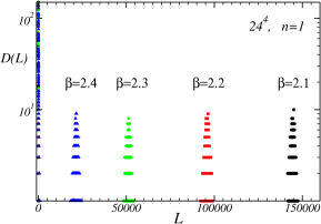
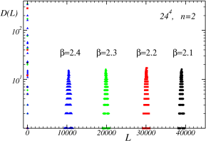
(a)	(b)

Figure 1: Distribution of the lengths of the monopole trajectories at various $\beta$ for (a) elementary and (b) $n=2$ blocked monopoles.

In Figure 1 we show the typical length distributions, $D(L)$, of the monopole trajectories in all clusters. We show the data for elementary, $n=1$, and blocked, $n=2$, monopoles at various lattice coupling constants $\beta$. One can see that for all considered values of the coupling $\beta$ the infrared cluster and the ultraviolet clusters can be unambiguously separated due to a wide gap between them. Moreover, the distributions of the elementary and blocked monopoles are qualitatively similar.

Note that at zero temperature the gap between IR and UV clusters becomes smaller as the physical lattice size decreases. This behaviour can be observed in Figure 1. At very small lattice size the gap between UV and IR clusters disappears and the IR and UV clusters can not be resolved. This behaviour of the monopole clusters leads to the deconfining transition (”crossover”) which takes place in sufficiently small physical volumes.

The distribution of the ultraviolet clusters was studied both numerically ref:hart ; zakharov:recent and analytically ref:zakharov:clusters ; ref:zakharov . The distribution can be described by a power law $D_{UV}\propto L^{-\tau}$, where the power $\tau$ is very close to 3, Ref. ref:hart . This behaviour indicates that the monopoles in UV clusters show a random walk picture ref:zakharov:clusters . In our simulations we are mainly concentrated on the IR monopole cluster because, as we have already mentioned in the Introduction, the IR cluster is important for the confinement of quarks. Below we study the monopole–related quantities using the largest monopole cluster only unless stated otherwise.

In general, the monopole action, $S^{{\mathrm{mon}}}_{{\mathrm{eff}}}$, can be represented as a sum of the $n$–point ($n\geq 2$) operators $S_{i}$, Ref. shiba:condensation ; chernodub :

$$S[k]=\sum_{i}f_{i}S_{i}[k]\,,$$ (14)

where $f_{i}$ are coupling constants. In this paper we adopt only the two–point interactions in the monopole action ($i.e.$ interactions of the form $S_{i}\sim k_{\mu}(s)k_{\mu^{\prime}}(s^{\prime})$). Following Ref. shiba:condensation we derive the effective monopole action (14) from the configurations of monopole currents, $\{k_{\mu}(s)\}$ using an inverse Monte-Carlo method. The original monopole configurations were generated by the usual Monte-Carlo algorithm of SU(2) gluodynamics.

The dominant term in the monopole action (14) corresponds to the most local self-interaction of the monopole currents, $S_{1}[k]=\sum_{s,\mu}k^{2}_{\mu}(s)$. The contributions to the action associated with other interactions are small compared to the leading term. As an example we show the leading contribution and the full action associated with the IR monopole cluster for $\beta=2.4$ and $n=1,2$ in Figure 2.

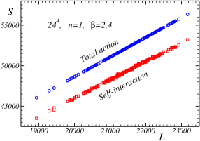
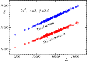
(a)	(b)

Figure 2: The total monopole action and the contribution of the self–interaction term to the action for (a) elementary and (b) $n=2$ extended monopoles $vs.$ length of the monopole trajectory in the IR cluster as calculated on $24^{4}$ lattice at $\beta=2.4$.

Moreover, one can find that both the monopole action and the self–coupling contribution to it are proportional with a good accuracy to the length of the monopole loop.

In Figure 3 we plot the ratio $S[k]/L$ for various lattice volumes and blocking sizes.

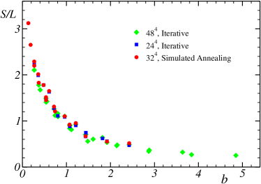
Figure 3: The ratio $S/L$, in physical units, as the function of $b$ for various lattices, $N^{4}$, and blocking steps, $n$.

One can notice that the coupling constant depends on the product $b=a\cdot n$ and almost does not depend on the variables $a$ and $n$ separately, in agreement with observations of Ref. shiba:condensation . Below we will observe this type of scaling in many other monopole quantities. Another observation is that the monopoles obtained with the SA procedure have the same action as the monopoles defined in the MA gauge which is fixed by the usual iterative algorithm.

It would also be interesting to compare the monopole action associated with the IR cluster and the action associated with the whole monopole ensemble. The simplest quantity to compare is the $f_{1}$ self–coupling parameter which is a dominant coupling in the action.

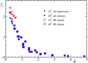
Figure 4: The self–interaction coupling constant $f_{1}$ as the function of $b$ calculated for the largest monopole cluster and for the whole monopole ensemble on lattices $24^{4}$ and $48^{4}$.

In Figure 4 we show $f_{1}$ for both ensembles. First, we easily notice that for chosen lattices the coupling constant $f_{1}$ is independent of the lattice volume. Second, we see that for large blocking scales $b$ the type of the ensemble (the IR cluster or the whole ensemble) is not essential for determination of $f_{1}$. However, at small $b$ values, $b\sqrt{\sigma}\lesssim 0.5$, the type of the lattice ensemble becomes important, since in this region

$$f^{\mathrm{IR}}_{1}>f^{\mathrm{total}}_{1}\,,\quad\mbox{for}\,\,\,\,b\sqrt{\sigma}\lesssim 0.5\,.$$ (15)

The observed difference between the couplings can be affected by finite–size effects since the leftmost points in our data correspond to elementary (of size $a$) monopoles. Moreover, in our studies we have included only the two–point interactions in the monopole action (14), while the two–point action becomes unreliable at too small values of $b$, and one has to include higher–point interactions.

Despite a possible influence of the lattice artifacts, the observation (15) may have a physical meaning related to the simple fact that the larger coupling $f_{1}$ the smaller density of the monopoles is. Thus Eq. (15) is in agreement with the numerical fact at large lattice coupling $\beta$ ($i.e.$, at small lattice spacing $a$) the density of the monopoles in the largest cluster is noticeably smaller than the total monopole density ref:bornyakov . Figure 4 is also in a qualitative agreement with the fact ref:anatomy that the excess of the Abelian action around elementary monopoles in all clusters and in the IR cluster almost coincide with each other. However, the larger the physical size of the monopole cube the better the agreement between the all–cluster and IR–cluster actions is, in accordance with Figure 4.

IV Monopole length distribution for IR cluster

As we have mentioned, the length distribution of the monopole trajectories in the ultraviolet clusters was found to obey the power–law. It would also be interesting to study the length distribution for the infrared clusters following Ref. ref:kitahara .

Since the density of the elementary monopoles from infrared clusters is finite (in terms of physical units) in the continuum limit ref:bornyakov , we may expect that the density of the extended monopoles (with a fixed blocking scale $b$) is finite as well. The finiteness of the density is consistent with the observation that the monopole length distribution is localized around a certain value of the monopole length, $L_{\mathrm{max}}$ (see Figure 1). This value should be proportional to the physical volume, $V$, of the system, $L_{max}\propto V$. Indeed, as one can qualitatively judge from Figure 1, the position of the peak of the IR length distribution increases with increase of the physical volume of the system ($i.e.$, with decrease of the lattice coupling $\beta$).

The length distribution function, $D(L)$, is proportional to the weight with which the particular trajectory of the length $L$ contributes to the partition function. On the other hand, the action of a monopole trajectory is proportional to the length of the trajectory, $S\propto L$, as we have illustrated in the previous Section. Thus the monopole action contributes in a form of an exponential factor, $\propto e^{-fL}$, to the weight with which this trajectory appears in the partition function. Here $f$ is a parameter which is close to the self-coupling $f_{1}$ according to Figure 4. The entropy of the monopole trajectory also contributes to the monopole length distribution, which is proportional to $\mu^{L}$ (with $\mu$ being positive number) for sufficiently large monopole lengths, $L$. Thus the distribution of the monopole trajectories in infinite volume must be described by the function

$$D^{IR}_{\inf}(L)\propto\mu^{L}\cdot e^{-f\,L}=e^{\gamma L}\,,\quad\gamma=\ln\mu-f\,.$$ (16)

In this equation we neglect a power-law prefactor which is essential for the distribution of the ultraviolet clusters ref:zakharov:clusters .

The observed localization of the infrared cluster distribution imply that the finite volume provide a certain cut which depends on the volume of the system. The simplest distribution of this kind can be described by the function:

$$D^{IR}(L)=\exp\{-\alpha L^{\eta}+\gamma L\}\,,$$ (17)

where $\alpha$, $\gamma$ and $\eta$ are certain parameters. As we find below, the parameter $\eta$ which characterizes the cut due to the volume effect, is close to 2 with a big accuracy, $\eta\approx 2$. Moreover, as we mentioned, the parameter $\gamma$ is characterizing the action and the entropy of the monopole currents and thus it should depend only of the physical size of the blocked monopole, $\gamma=\gamma(b)$. As for the parameter $\alpha$, it should also be dependent of the volume of the system, $\alpha=\alpha(b,V)$. Thus we employ the following parameterization of the IR monopole distribution at finite volume:

$$D^{IR}(L)=\exp\{-\alpha(b,V)L^{2}+\gamma(b)L\}\,.$$ (18)

The peak of the distribution (18),

$$L_{max}=\frac{\gamma(b)}{2\,\alpha(b,V)}\,,$$ (19)

is expected to be proportional to the volume of the system, $L_{max}\propto V$ to insure the finiteness of the IR monopole density,

$$\rho_{IR}=\frac{L_{max}}{V}=\frac{\gamma(b)}{2\,\alpha(b,V)\,V}\,,$$ (20)

in the thermodynamic limit, $V\to\infty$. Thus from Eq.(20) we conclude that

$$\alpha(b,V)=A(b)/V\,,$$ (21)

where the function $A(b)$ depends only on the size of the blocked monopole, $b$. Eq.(21) implies that in the thermodynamic limit the parameter $\alpha$ vanishes and the finite–volume distribution (17) is reduced to Eq.(16), as expected.

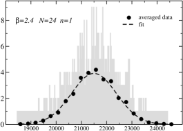
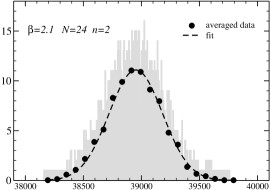
(a)	(b)

Figure 5: The original histograms of the length distribution in the IR cluster are shown by grey color. The averaged distributions are shown by circles, and the fits by the function (18) are represented by the dashed line.

We show typical examples of the IR cluster distributions in Figure 5 by grey color. One can see that these histograms have an almost symmetric structure, but due to the lack of statistics these histograms can not be fitted by the function (18). In order to show that the distribution of the monopole follows Eq.(18) we smooth the data by increasing the step of the histograms (which was equal to $2$) and then averaging the data inside the coarse steps. We show the averaged (and suitably rescaled) histograms and their fits by the function (18) in the same Figure. One can see that the averaged histograms are very close to the Gaussian distribution. Similar behaviour can also be observed for all IR monopole cluster distributions we have studied in this paper.

In order to justify the chosen value of the parameter $\eta$ in Eq. (18) we have also fitted the averaged histogram data by Eq. (17) in which $\eta$ is treated as a fitting parameter. The best fit (for $\beta=2.4$ and $n=1$ on $24^{4}$ lattice, as an example) gives us the result $\eta=2.05(15)$. Fits of other histograms give us similar results. Thus we fix below $\eta=2$.

The histograms in Figure 5 were obtained with a high simulation statistics (3000 configurations according to Table 1). In order to get a perfect gaussian we would need much more statistics which would consume a lot of CPU time. To avoid this we assume that the numerical data for length distribution of the IR monopoles is described by Eq.(18). This assumption is justified by the analysis we have performed above. Then one can evaluate the central values of the parameters $\alpha$ and $\gamma$ using the simple formulae (valid for a Gaussian distribution):

$$\alpha=\frac{1}{2}\frac{1}{\langle L^{2}\rangle-\langle L\rangle^{2}}\,,\quad\gamma=\frac{\langle L\rangle}{\langle L^{2}\rangle-\langle L\rangle^{2}}\,,$$ (22)

where the averaging $\langle\cdots\rangle$ is performed using weights from the histograms.

To evaluate the errors for the parameters $\alpha$ and $\gamma$ we use the standard bootstrap method. Namely, we make a resampling of the original data describing lengthes of the IR monopole clusters, $L_{\max}$. We construct a resampled configuration by selecting $n_{conf}$ random values of $L_{\max}$ (note that a single value of $L_{\max}$ can be picked up multiple number of times), where $n_{conf}$ is the total number of the monopole configurations. Then we evaluate the values of $\alpha$ and $\gamma$ at each resampled configuration using Eq. (22). The distribution of these values is again the Gaussian with the width equal to the corresponding error. We plot examples of the histograms for $\alpha$ and $\gamma$ values in Figures 6(a,b).

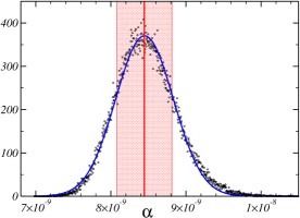
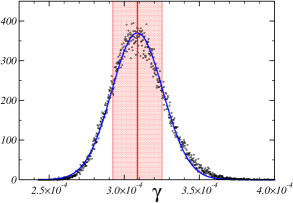
(a)	(b)

Figure 6: The distribution of the parameter $\alpha$ and $\gamma$ for elementary monopoles at $\beta=2.4$ on $24^{4}$ lattice. The fits by a gaussian function are shown by the solid lines and the value of the errors are indicated by shadowed regions.

We have checked the applicability of Eqs. (22) and the use of the bootstrap method on a smaller, $16^{4}$, lattice. Namely, we have generated length distributions using from low statistics ($2000$ configurations) to high statistics ($10^{5}$ configurations) ensembles. We used the bootstrap method along with Eqs. (22) to evaluate the coefficients $\alpha$ and $\beta$ for the distribution measured with the lowest statistics. On the other hand, the high statistics distribution is a (almost perfect) Gaussian and therefore we get the desired coefficients directly from the fit (18). The comparison of the coefficients shows that the central values as well as the estimated errors for the low and for the high statistics ensembles coincide with each other within a few percents. We illustrate our analysis in Figure 7 for $\beta=2.1$ and $\beta=2.2$ using the parameter $\gamma$ as an example. The values of $\gamma$ obtained with the standard method are plotted $vs.$ number of configurations, $N_{conf}$, used in the analysis. The horizontal lines represent the results coming from the bootstrap method applied to the low-statistic ensemble (the statistical errors are indicated by shadowed regions). We conclude that the bootstrap method allows to get reliable results using the distributions with low–statistics.

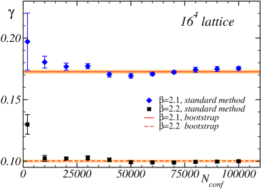
Figure 7: Check of the bootstrap method on $1643$ lattice using the parameter $\gamma$ as an example (the explanation is in the text).

In order to confirm our expectation (21) we plot the parameter $\alpha$ $vs.$ the ratio $N/n$ in Figure 8(a) for selected set of coupling constants $\beta$ and the blocking steps of the monopole, $n$. Since the volume of the blocked lattice is ${(N/n)}^{4}$, we expect that the parameter $\alpha$ behaves as $\alpha\propto{(N/n)}^{-4}$. This behaviour is seen in Figures 8(a,b). The parameter $\alpha$ multiplied by the lattice volume almost does not depend on the lattice size $N$ according to Figure 8(b).

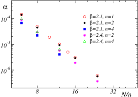
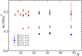
(a)	(b)

Figure 8: (a) The fitting parameter $\alpha$ as the function of the size $N/n$ of the coarse lattice; (b) the parameter $\alpha$ multiplied by the lattice volume as the function of the lattice size $N$.

According to our discussion above the fitting parameter $\gamma$ should only be a function of the blocking size $b$ and should not depend on the volume of the lattice. In Figure 9 we show the parameter $\gamma$ is indeed independent of the lattice size $N$.

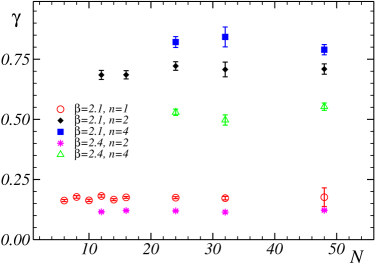
Figure 9: The illustration of the independence of the fitting parameter $\gamma$ on the lattice size, $N$.

The fitting parameters $\alpha$ and $\gamma$ are shown as functions of the physical scale $b$ in Figures 10(a) and (b), respectively. The parameter $\gamma$ shows the scaling behaviour in a sense that it depends on the blocking step $n$ and lattice spacing $a$ in the form of the product $b=n\cdot a$.

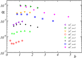
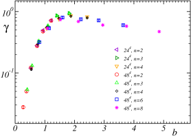
(a)	(b)

Figure 10: The fitting parameters (a) $\alpha$ and (b) $\gamma$ as functions $b$ for various lattice volumes, $N^{4}$, and monopole blocking steps, $n$.

V Monopole density and entropy

V.1 Monopole density

The simplest physical characteristic of the monopole ensemble is its density. It is interesting to compare the monopole density obtained from the IR monopole cluster distribution, Eq. (20), with the direct observation of the monopole density,

$$\rho_{IR}=\frac{1}{4{(na)}^{3}\cdot(N/n)^{4}}\Bigl{\langle}\sum_{s,\mu}|k^{(n)}_{\mu}(s)|\Bigr{\rangle}\,.$$ (23)

Here the blocked monopole current, $k^{(n)}_{\mu}$, is defined by Eq. (10). The normalization factor in Eq. (23) appears naturally if one notes that $b=na$ and $4(N/n)^{4}$ are the lattice spacing and the number of links of the coarse lattice, respectively.

If the fitting function (18) describes the data correctly then one should observe no essential difference between the infrared monopole density obtained from the fits of the monopole distributions, (18,20) compared to the density obtained in a direct way (23). This is indeed the case according to Figure 11(a).

Another information which can be extracted from this Figure is that the blocked monopole density goes to a fixed limit, $\lim_{b\to 0}\rho\approx 0.9\,\sigma^{3/2}$, as the blocking size $b$ gets smaller. It is also possible that the monopole density shows a wide plateau around $b\sqrt{\sigma}\approx 0.2$. In order to discriminate between these options one should study the blocked monopole density at smaller values of lattice spacing, $a$, and, consequently, at larger lattice volumes. We also note that the value of the blocked monopole density quoted above is about $30\%$ larger than the value of density ref:bornyakov of the elementary infrared monopoles in the continuum limit.

The monopole density is known to be sensitive to the details of the gauge fixing procedure ref:bornyakov . In order to check the effect of the gauge fixing we compare in Figure 11(b) the infrared monopole density obtained using the SA and iterative gauge fixing algorithms. One can see from this Figure that at large $b$ there is practically no difference between the monopole densities obtained with the use of the different algorithms. However, there exists some difference at small $b$ since the SA monopole density is smaller than the density obtained with the help of the iterative algorithm. This slight dependence of the density on the gauge fixing algorithm at small $b$ may explain the discrepancy between our results and the results of Ref. ref:bornyakov mentioned above. Another source of the discrepancy is the qualitative difference between the elementary and the blocked monopoles. Since the scale $b$ is taken to be independent of the lattice spacing $a$ while $a$ tends to zero in the continuum limit, the elementary monopoles are expected to be more affected by the ultraviolet lattice artifacts.

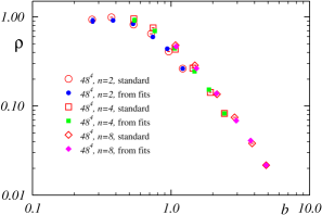
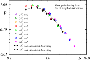
(a)	(b)

Figure 11: (a) Comparison of the infrared monopole density obtained from the fits of the monopole distributions, (18,20) with the density obtained in a direct way (23). (b) Comparison of the effect of the gauge fixing procedure (iterative $vs.$ simulated annealing) on the infrared monopole density.

V.2 Monopole entropy

The distribution of the monopole trajectories depends both on the monopole action and on the monopole entropy as we have already discussed in Section IV. Therefore the knowledge of the distribution and the monopole action allows us to define the entropy of the monopole currents. If the monopoles make a simple random walk on the four–dimensional hypercubic lattice then the entropy factor for elementary monopoles is expected to be equal to seven, $\mu=7$, since there are seven choices at each site for the monopole current to go further (the monopole trajectory is obviously non–backtracking due to the presence of the magnetic charge).

The balance between energy and entropy of the elementary monopole trajectories plays an important role. For example, the compact U(1) gauge model in four dimensions possesses a phase transition associated with the monopole (de)condensation which is defined as a point on the phase diagram where the entropy and the energy of the monopole trajectories are the same. This point is located by the condition $\gamma=0$, where $\gamma$ characterizes the monopole distribution, Eq. (16) or (18).

In the case of the compact $U(1)$ gauge model the coefficient $f$ in the action of the monopole trajectory, $S=fL$, is proportional to the lattice gauge coupling, $f_{U(1)}\propto\beta_{U(1)}$ and $\mu=7$. This fact allowed authors of Ref. ref:BMK to find the critical value of $\beta_{U(1)}$ deconfinement transition point with a great accuracy. Indeed, if $\gamma$ is negative then the infrared cluster disappears and the confinement of electric charges is lost. The energy-entropy balance was also studied numerically for the monopoles in compact U(1) gauge theory ref:suzuki:shiba and in finite–temperature pure SU(2) gauge theory ref:kitahara .

In the pure zero temperature QCD the coupling $\gamma$ is positive at all values of the lattice coupling constant $\beta$. The approximate cancellation of the entropy factor and the energy of the elementary monopoles in the zero–temperature gluodynamics is known as ”fine tuning” ref:zakharov:clusters ; ref:zakharov . This fact is in agreement with the existence of physical scaling of the infrared cluster in zero–temperature pure QCD.

The entropy factor $\mu$ of the infrared monopole trajectories can be obtained from the IR cluster distribution and the monopole action according to Eq. (16),

$$\mu=e^{\gamma+f}\,.$$ (24)

We calculate numerically the parameters $\gamma$ and $f$ to find the entropy factor $\mu$ for various scales $b$ and lattice sizes. Our results are presented in Figure 12. The entropy shows an approximate scaling behaviour in a sense that the entropy depends only on the scale $b$ and is independent of the lattice spacing, $a$, and the blocking factor, $n$, separately. One can also notice that the entropy $\mu$ is independent of the volume of the lattice. The largest scaling violations happens at small blocking sizes $n=1,2$ at which the finite–size artifacts are expected to be strong.

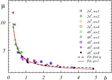
Figure 12: Entropy factor $\mu$ $vs.$ $b$. The dashed line represents the fit by Eq. (25) with free $q$–parameter and the solid line corresponds to the fixed parameter, $q=1$.

The entropy factor $\mu$ is a declining function of the scale $b$. According to discussion above one can expect that for elementary monopoles the factor $\mu$ should be equal to seven. However, $\mu>7$ for small values of $b$, as can be seen from Figure 12. We explain this small–$b$ behaviour as an artifact of our numerical procedure adopted in this paper. Indeed, we have used the quadratic monopole action while at small $b$ higher–point interaction terms are essential and thus the monopole action can not be reliably described by the quadratic terms only chernodub .

At large $b$ the entropy factor (24) is smaller than seven. Formally this means that the motion of the blocked monopoles is constrained. We have fitted the entropy by the function:

$$\mu^{\mathrm{fit}}=\mu_{\infty}+C\,\mu^{-q}\,,$$ (25)

where $\mu_{\infty}$, $C$ and $q$ are the fitting parameters. The best fit is shown in Figure 12 by the dashed line. The corresponding best fit parameters are: $\mu_{\infty}=1.6(4)$, $C=1.7(5)$ and $q=1.2(2)$. The most interesting fitting parameter is $\mu_{\infty}$ which is the asymptotic value of the entropy in the infrared limit $b\sigma^{1/2}\to\infty$ according to Eq. (25). Unfortunately, the value of the asymptotic entropy is obtained with a big error bar in the above fit. In order to increase the accuracy we notice that the power $q$ is very close to unity. Fixing $\mu=1$ in Eq. (25) and repeating the fitting procedure again we get $\mu_{\infty}=1.15(25)$ and $C=2.2(1)$. The corresponding best fit curve is shown in Figure 12 by the solid line.

The fact that the asymptotic value of the entropy is very close to the unity in the limit $b\sigma^{1/2}\to\infty$ may have a simple explanation. The monopole with a large blocking size $b$ behaves as a classical object and its motion is no more a simple random walk. The predominant motion of the large–$b$ monopole is close to a straight line.

VI Conclusion

We studied numerically the distributions of the infrared monopole currents of various blocking sizes, $n$, on the lattices with different spacings, $a$, and volumes, $N$. The distributions can be described by a gaussian anzatz with a good accuracy. The anzatz contains two important terms: (i) the linear term, which possesses information about the energy and entropy of the monopole currents; and (ii) the quadratic term, which suppresses too large infrared clusters. The linear term is independent of the lattice volume while the quadratic term is inversely proportional to the volume. The monopole density determined from the parameters of the gaussian fits coincides with the result of the direct numerical calculation.

We also studied the action of the monopoles belonging to the infrared clusters and compared it with the action of the total monopole ensemble. It turns out that the self–coupling coefficients for both these ensembles are almost the same at large $b$. However, as the blocking scale $b$ is decreased the self–coupling coefficient for infrared monopole cluster gets noticeably larger then the coefficient for the total monopole ensemble. This can be explained by the fact that the self-interaction coefficient depends on the monopole density (the larger density the smaller the coefficient is), and the difference between the total density and the infrared density increases as $b$ gets smaller.

The knowledge of both the coefficient in front of the linear term of the gaussian distribution and the monopole action for infrared clusters allows us to determine the entropy factor of the extended (blocked) monopole currents. We have numerically shown that the entropy of the blocked monopole currents is a descending function of $b=na$, indicating that the effective degrees of freedom of the blocked monopoles are getting smaller as the blocking scale $b$ increases. This corresponds to the classical picture: the monopole with the large blocking size $b$ becomes a macroscopic object and the motion of such a monopole is close to a straight line.

- (1) G. ’t Hooft, in High Energy Physics, ed. A. Zichichi, EPS International Conference, Palermo (1975); S. Mandelstam, Phys. Rept. 23, 245 (1976).
- (2) G. ’t Hooft, Nucl. Phys. B190, 455 (1981).
- (3) T. Suzuki, Nucl. Phys. Proc. Suppl. 30, 176 (1993); M. N. Chernodub and M. I. Polikarpov, “Abelian projections and monopoles”, in ”Confinement, duality, and nonperturbative aspects of QCD”, Ed. by P. van Baal, Plenum Press, p. 387, hep-th/9710205; R.W. Haymaker, Phys. Rept. 315, 153 (1999).
- (4) H. Shiba and T. Suzuki, Phys. Lett. B 351, 519 (1995).
- (5) N. Arasaki, S. Ejiri, S. i. Kitahara, Y. Matsubara and T. Suzuki, Phys. Lett. B 395, 275 (1997); M. N. Chernodub, M. I. Polikarpov, A. I. Veselov, Phys. Lett. B 399, 267 (1997); Nucl. Phys. Proc. Suppl. 49, 307 (1996); A. Di Giacomo and G. Paffuti, Phys. Rev. D 56, 6816 (1997).
- (6) H. Shiba and T. Suzuki, Phys. Lett. B 333, 461 (1994);
- (7) T. Suzuki and I. Yotsuyanagi, Phys. Rev. D42, 4257 (1990); G. S. Bali, V. Bornyakov, M. Müller-Preussker and K. Schilling, Phys. Rev. D54, 2863 (1996).
- (8) Y. Koma, M. Koma, E. M. Ilgenfritz, T. Suzuki and M. I. Polikarpov, “Duality of gauge field singularities and the structure of the flux tube in Abelian-projected SU(2) gauge theory and the dual Abelian Higgs model”, hep-lat/0302006.
- (9) T.L. Ivanenko, A.V. Pochinsky, M.I. Polikarpov, Phys. Lett. B 252, 631 (1990).
- (10) S. Kitahara, Y. Matsubara, T. Suzuki, Progr. Theor. Phys. 93, 1 (1995).
- (11) A. Hart, M. Teper, Phys. Rev., B58, 014504 (1998).
- (12) P. Y. Boyko, M. I. Polikarpov and V. I. Zakharov, “Geometry of percolating monopole clusters”, hep-lat/0209075.
- (13) M. N. Chernodub and V. I. Zakharov, Towards understanding structure of the monopole clusters, hep-th/0211267.
- (14) V.G. Bornyakov, P.Yu. Boyko, M.I. Polikarpov, V.I. Zakharov, “Monopole clusters at short and large distances”, hep-lat/0305021.
- (15) A. S. Kronfeld, M. L. Laursen, G. Schierholz and U. J. Wiese, Phys. Lett. B 198, 516 (1987); A. S. Kronfeld, G. Schierholz and U. J. Wiese, Nucl. Phys. B 293, 461 (1987).
- (16) T. A. DeGrand and D. Toussaint, Phys. Rev. D 22, 2478 (1980).
- (17) G. S. Bali, V. Bornyakov, M. Muller-Preussker and K. Schilling, Phys. Rev. D 54 (1996) 2863.
- (18) V. I. Zakharov, “Hidden Mass Hierarchy in QCD”, hep-ph/0202040
- (19) M. N. Chernodub, S. Fujimoto, S. Kato, M. Murata, M. I. Polikarpov and T. Suzuki, Phys. Rev. D 62, 094506 (2000); M. N. Chernodub, S. Kato, N. Nakamura, M. I. Polikarpov and T. Suzuki, “Various representations of infrared effective lattice SU(2) gluodynamics”, hep-lat/9902013.
- (20) V. Bornyakov and M. Muller-Preussker, Nucl. Phys. Proc. Suppl. 106, 646 (2002).
- (21) V. G. Bornyakov, M. N. Chernodub, F. V. Gubarev, M. I. Polikarpov, T. Suzuki, A. I. Veselov and V. I. Zakharov, Phys. Lett. B 537, 291 (2002).
- (22) T. Banks, R. Myerson and J. B. Kogut, Nucl. Phys. B 129, 493 (1977).
- (23) H. Shiba and T. Suzuki, Phys. Lett. B 343, 315 (1995).