$B\to\pi$ and $B\to K$ transitions in partially quenched chiral perturbation theory

Abstract

We study the properties of the $B\to\pi$ and $B\to K$ transition form factors in partially quenched QCD by using the approach of partially quenched chiral perturbation theory combined with the static heavy quark limit. We show that the form factors change almost linearly when varying the value of the sea quark mass, whereas the dependence on the valence quark mass contains both the standard and chirally divergent (quenched) logarithms. A simple strategy for the chiral extrapolations in the lattice studies with ${N_{\rm sea}}=2$ is suggested. It consists of the linear extrapolations from the realistically accessible quark masses, first in the sea and then in the valence quark mass. From the present approach, we estimate the uncertainty induced by such extrapolations to be within $5\%$.

I Introduction

In order to extract the Cabibbo-Kobayashi-Maskawa matrix element $|V_{ub}|$ from the experimentally measured decay rate for $B\to\pi\ell\nu_{\ell}$ at Belle and BaBar, a reliable theoretical prediction of the corresponding hadronic matrix element is indispensable. Two major sources of systematic uncertainty in the current lattice QCD calculations of the $heavy\to light$ pseudoscalar meson transitions are the quenched approximation and the errors associated with the chiral extrapolations. All the available results of the lattice studies of the semileptonic $B\to\pi$ decay are obtained in the quenched approximation ($N=0$) and by working with light quark masses larger than $m_{s}^{phys}/2$ lattice .

Since fully unquenched QCD lattice simulations (i.e., with $N=3$) are not feasible it is important to have a method to assess whether or not a given physical quantity is prone to large quenching errors. With such an ambition in mind, Sharpe sharpe , and later Bernard and Golterman bernard , formulated the quenched chiral perturbation theory (QChPT). By confronting the predictions derived in QChPT with those obtained in the full chiral perturbation theory (ChPT), one gets a rough estimate on the size of quenching errors. The approach has been extended to the heavy-light quark systems by combining ChPT and the heavy quark effective theory (HQET) booth ; zhang . The effect of complete quenching on the lattice determination of the $B\to\pi$ form factors has been studied recently by the present authors in Ref. JSD, . It has been found that the quenching errors on the $B\to\pi$ and $B\to K$ transition form factors may be uncomfortably large (typically larger than $20\%$). This conclusion somewhat spoils the significance of the impressive agreement that has been reached amongst various lattice groups using different lattice techniques to compute $B\to\pi$ decay in the quenched approximation lattice .

It is therefore highly important to perform the simulations in which the effects of dynamical quarks are included. A step in that direction is to implement the partial quenching, i.e., to include in the simulation $N_{\rm sea}$ dynamical light quarks with masses generally different from those of the valence quarks. The lattice studies with $N_{\rm sea}=2$ are likely to be performed first, which is the main motivation for the present work.

We calculate the form factors for $B\to\pi$ and $B\to K$ transitions in partially quenched chiral perturbation theory (PQChPT) Bernard:1993sv ; Damgaard:1998xy ; Sharpe:2001fh , combined with HQET zhang . We work in the static heavy quark limit and at next-to-leading order (NLO) of the chiral expansion. This approach is valid for small recoil momenta ($v\negmedspace\cdot\negmedspace p$), i.e., the same one currently accessible from the lattice simulations. We limit ourselves to the case of ${N_{\rm sea}}$ degenerate sea quarks of mass ${m_{\rm sea}}$. On the basis of our calculation we conclude that the dependence of the form factors on the sea quark mass is essentially linear, and that the form factors are finite as ${m_{\rm sea}}\to 0$ when ${m_{\rm val.}}$ is non-zero. On the other hand, the limit ${m_{\rm val.}}\to 0$, with ${m_{\rm sea}}\neq{m_{\rm val.}}$, is not well defined, since in this case the form factors contain the chirally divergent “quenched” logarithmic terms ${m_{\rm sea}}\ln{m_{\rm val.}}$. Our analysis of PQChPT with ${N_{\rm sea}}=2$ shows that a simple linear chiral extrapolation first in the sea quark mass, ${m_{\rm sea}}$, and then in the valence quark mass, ${m_{\rm val.}}$, introduces an extrapolation error of only $5\%$, where the linear extrapolations are made from the range of the quark masses that are currently accessible in the lattice simulations. Furthermore, by assuming that the low energy constants in the full ChPT with $N=2$ and $N=3$ are equal, we deduce the residual quenching errors of lattice studies with ${N_{\rm sea}}=2$ to be in the ball park of $10-20\%$. Those two conclusions indicate that, in comparison with the fully quenched simulation, the additional computational cost of making the partial unquenching (with ${N_{\rm sea}}=2$) is well worth the effort.

The remainder of this paper is organized as follows. In Sec. II we remind the reader about the elements of the PQChPT and set our notation. In Sec. III we present the results of the NLO calculation in PQChPT for $B\to\pi(K)$ form factors. The quenching errors and chiral extrapolation formulas are discussed in Sec. IV. Main conclusions are shortly stated in Sec. V.

II Partially quenched chiral perturbation theory

In this section we make a succinct summary of PQChPT. We consider partially quenched QCD with $N_{\rm sea}$ sea quarks degenerate in mass (${m_{\rm sea}}$), and with two valence quarks $q_{a}$ and $q_{b}$ of masses $m_{a}$ and $m_{b}$, respectively. Partial quenching is introduced by adding bosonic “ghost”-quarks $\tilde{q}_{a,b}$ of spin $\tfrac{1}{2}$ and mass $m_{a,b}$, which cancel the fermion loops of valence quarks sharpe ; bernard ; Bernard:1993sv ; morel . Assuming the spontaneous symmetry breaking pattern to be the same as in full QCD Sharpe:2001fh , the leading-order Lagrangian for the (pseudo) Goldstone bosons is Bernard:1993sv ; Damgaard:1998xy ; Sharpe:2001fh

$${\cal L}_{\rm light} = {f^{2}\over 8}\operatorname{str}\left(\partial_{\mu}\Sigma\partial^{\mu}\Sigma^{\dagger}\right)+{f^{2}\mu_{0}\over 2}\operatorname{str}({\cal M}\Sigma+{\cal M}\Sigma^{\dagger})$$ (2)

$$+{\cal L}_{4}\,,$$

with $f\approx 130$ MeV, $\operatorname{str}(U)={\displaystyle{\sum_{i}}}U_{ii}\epsilon_{i}$, and

$$\epsilon_{i} = \operatorname{diag}(\underbrace{1,\dots,1}_{N_{\rm sea}+2},-1,-1),$$ (3)

$${\cal M} = \operatorname{diag}(m_{a},m_{b},\underbrace{{m_{\rm sea}},\dots,{m_{\rm sea}}}_{N_{\rm sea}},m_{a},m_{b}),$$ (4)

while

$$\Sigma=\exp\left(2i\frac{\Phi}{f}\right),\qquad\Phi=\begin{pmatrix}\phi&\chi^{\dagger}\\ \chi&\tilde{\phi}\;\end{pmatrix}\;.$$ (5)

The graded ${\rm SU}(2\!+\!N_{\rm sea}|2)$ matrix $\Phi$ contains a $[(2+N_{\rm sea})\times(2+N_{\rm sea})]$ matrix $\phi$ of quark–anti-quark bosons, a $[2\times 2]$ matrix $\tilde{\phi}$ of ghost–anti-ghost bosons, and the matrices of pseudoscalar fermions, $\chi^{\dagger}\sim\bar{\tilde{q}}q$ and $\chi\sim\bar{q}\tilde{q}$. In this framework the heavy $\eta^{\prime}$ has been integrated out ($m_{0}\to\infty$) in a way similar to the full ChPT. This is to be contrasted to the fully quenched theory, where the $\eta^{\prime}$ cannot be integrated out. The propagators of the “off-diagonal” and “diagonal” mesons ($\Phi_{ab}\sim\bar{q}_{a}q_{b}$) are given respectively by

$$\langle\Phi_{ab}|\Phi_{ba}\rangle_{a\not=b}=i\frac{\epsilon_{a}}{p^{2}-M_{ab}^{2}},$$ (6)

$$\langle\Phi_{aa}|\Phi_{bb}\rangle=i\biggl{[}\frac{\delta_{ab}\epsilon_{a}}{p^{2}-M_{aa}^{2}}-\frac{1}{N_{\rm sea}}\frac{p^{2}-M_{S}^{2}}{(p^{2}-M_{aa}^{2})(p^{2}-M_{bb}^{2})}\biggr{]},$$ (7)

with $M_{ab}^{2}=2\mu_{0}(m_{a}+m_{b})$, and $M_{S}^{2}=4\mu_{0}{m_{\rm sea}}$.

Since PQChPT with $N_{\rm sea}=3$, and $m_{a}=m_{b}\equiv{m_{\rm sea}}$ coincides with the full ChPT with $m_{u}=m_{d}=m_{s}$, the corresponding low energy constants obtained in the two theories are equal.  Since the low energy constants do not depend on the quark masses, the mentioned equality among low energy constants persists even when the valence and sea quark masses of partially quenched theory are not of the same size Sharpe:2001fh . On the other hand the low energy constants do depend on the number of dynamical quark flavors and therefore the equality holds only for $N_{\rm sea}=3$.

The two terms appearing at NLO in the effective Lagrangian (2) relevant to $B\to\pi$ and $B\to K$ form factors are

$${\cal L}_{4} = 4\mu_{0}\Big{\{}L_{4}\operatorname{str}\left(\partial_{\mu}\Sigma\partial^{\mu}\Sigma^{\dagger}\right)\operatorname{str}\left({\cal M}\Sigma^{\dagger}+\Sigma{\cal M}^{\dagger}\right)$$ (10)

$$+L_{5}\operatorname{str}\left[\partial_{\mu}\Sigma^{\dagger}\partial^{\mu}\Sigma\left({\cal M}\Sigma^{\dagger}+\Sigma{\cal M}^{\dagger}\right)\right]+\cdots\Big{\}}~{}.\;$$

It is straightforward to verify that Eq. (2) leads to the standard, full QCD, chiral Lagrangian after setting $\operatorname{str}\to\operatorname{tr}$, $\Phi\to\phi$ (for a review of ChPT see Ref. Donoghue:dd, or any paper listed in Ref. chiral-reviews, ).

II.1 Incorporating the heavy quarks

To extend the applicability of the Lagrangian (2) to the heavy-light mesons, the heavy quark spin symmetry needs to be included. This is achieved by combining the pseudoscalar ($P^{a}$) and vector ($P^{\ast\ a}_{\mu}$) heavy-light mesons in one field:

$$H_{a}(v) = {1+v\kern-5.75pt\raise 0.6458pt\hbox{/}\over 2}\left[P^{\ast\ a}_{\mu}(v)\gamma_{\mu}-P^{a}(v)\gamma_{5}\right]~{},$$ (11)

$$\overline{H}_{a}(v) = \gamma_{0}H_{a}^{\dagger}(v)\gamma_{0}\;.$$ (12)

We also introduce the covariant derivative and the axial field as

$$D_{\mu}^{ba}H_{b} = \partial_{\mu}H_{a}-H_{b}{1\over 2}[\xi^{\dagger}\partial_{\mu}\xi+\xi\partial_{\mu}\xi^{\dagger}]_{ba}~{},$$ (13)

$${\bf A}_{\mu}^{ab} = {i\over 2}[\xi^{\dagger}\partial_{\mu}\xi-\xi\partial_{\mu}\xi^{\dagger}]_{ab}\;,$$ (14)

where $a$ and $b$ run over the light quark flavors, and $\xi=\sqrt{\Sigma}$. Finally, the partially quenched chiral Lagrangian for the heavy-light mesons in the static heavy quark limit reads booth ; zhang

$${\cal L}_{\rm heavy} = -\operatorname{str}_{a}\operatorname{Tr}[\overline{H}_{a}iv\negmedspace\cdot\negmedspace D_{ba}H_{b}]$$ (17)

$$+g\operatorname{str}_{a}\operatorname{Tr}[\overline{H}_{a}H_{b}\gamma_{\mu}{\bf A}_{ba}^{\mu}\gamma_{5}]+{\cal L}_{3}\;,$$

where $g$ is the coupling of the heavy meson doublet to the Goldstone boson. The higher order terms in the expansion in $v\negmedspace\cdot\negmedspace p$ and in $m_{q}$ [${\cal O}(p^{2})$] have the following form booth ; JSD :

$${\cal L}_{3} = 2\lambda_{1}\operatorname{str}_{a}\operatorname{Tr}[\overline{H}_{a}H_{b}]({\cal M_{+}})_{ba}$$ (22)

$$+k_{1}\operatorname{str}_{a}\operatorname{Tr}[\overline{H}_{a}iv\negmedspace\cdot\negmedspace D_{bc}H_{b}]({\cal M_{+}})_{ca}$$

$$+k_{2}\operatorname{str}_{a}\operatorname{Tr}[\overline{H}_{a}iv\negmedspace\cdot\negmedspace D_{ba}H_{b}]\operatorname{str}_{c}({\cal M_{+}})_{cc}+\dots\;,$$

with ${\cal M_{+}}={1\over 2}(\xi^{\dagger}M\xi^{\dagger}+\xi M\xi)$. We again display only the terms that contribute to the heavy-to-light form factors of $B\to\pi,K$ transitions. In the above equations, “Tr” stands for the trace over Dirac indices, whereas “str” is the super-trace over the light flavor indices. The standard chiral Lagrangian for heavy-light mesons reviews-HQChPT ; burdman is recovered by replacing $\operatorname{str}\to\operatorname{tr}$, $\Phi\to\phi$.

The bosonized heavy $\to$ light weak current $(V-A)$, in the static heavy quark limit and at NLO in the chiral expansion, reads booth ; JSD

$$\begin{split}J^{\mu}\equiv\bar{q}_{a}\gamma^{\mu}(1-\gamma_{5})Q&\to\frac{i\alpha}{2}\operatorname{Tr}[\gamma^{\mu}(1-\gamma_{5})H_{b}]\xi_{ba}^{\dagger}\\ &+\frac{i\alpha}{2}\varkappa_{1}\operatorname{Tr}[\gamma^{\mu}(1-\gamma_{5})H_{c}]\xi_{ba}^{\dagger}({\cal M_{+}})_{cb}\\ &+\frac{i\alpha}{2}\varkappa_{2}\operatorname{Tr}[\gamma^{\mu}(1-\gamma_{5})H_{b}]\xi_{ba}^{\dagger}\operatorname{str}_{c}({\cal M_{+}})_{cc}\;.\end{split}$$ (23)

The phase of the heavy meson can be chosen in such a way that the constants $\alpha$, $\varkappa_{1}$ and $\varkappa_{2}$ are real. At the leading order in the chiral expansion, the constant $\alpha$ is proportional to the heavy-light meson decay constant, $\alpha=\sqrt{m_{B}}f_{B}$.

II.2 Form factors

The standard decomposition of the vector current matrix element between two pseudoscalar meson states is

$$\langle P(p)|\bar{q}\gamma_{\mu}b|B(p_{B})\rangle = \left[(p_{B}+p)_{\mu}-q_{\mu}{m_{B}^{2}-m_{P}^{2}\over q^{2}}\right]F_{+}(q^{2})$$ (25)

$$+{m_{B}^{2}-m_{P}^{2}\over q^{2}}q_{\mu}F_{0}(q^{2})\;,$$

where the form factors $F_{+,0}$ are functions of the momentum transfer squared $q^{2}=(p_{B}-p)^{2}$. A light meson $P$ stands for $\pi$, $K$ with the light quark in the current being $q=d,s$, respectively.

We work in the static limit ($m_{B}\to\infty$) in which the eigenstates of QCD and HQET Lagrangians are related through ${1\over\sqrt{m_{B}}}|B(p_{B})\rangle_{\rm QCD}=|B(v)\rangle_{\rm HQET}$. In the static limit it is more convenient to use a definition in which the form factors are independent of the heavy meson mass. We will use

$$\langle P(p)|\bar{q}\gamma_{\mu}b_{v}|B(v)\rangle_{\rm{HQET}} = \bigl{[}p_{\mu}-(v\negmedspace\cdot\negmedspace p)v_{\mu}\bigr{]}f_{p}(v\negmedspace\cdot\negmedspace p)$$ (27)

$$+\ v_{\mu}f_{v}(v\negmedspace\cdot\negmedspace p)\;,$$

where the field $b_{v}$ does not depend on the heavy quark mass. The form factors $f_{p,v}$ are functions of the variable

$$v\negmedspace\cdot\negmedspace p={m_{B}^{2}+m_{P}^{2}-q^{2}\over 2m_{B}}\;,$$ (28)

which is the energy of the light meson $E_{P}$, in the heavy meson rest frame. The relation between the quantities defined in Eqs. (25) and (27) is obtained by matching QCD to HQET at the scale $\mu\sim m_{b}$ hill . By setting the matching constants to their tree level values and neglecting the subleading terms in the heavy quark expansion, one has

$$\Biggl{.}F_{0}(q^{2})\Biggr{|}_{q^{2}\approx q^{2}_{\rm max}}={1\over\sqrt{m_{B}}}f_{v}(v\negmedspace\cdot\negmedspace p)\;,$$ (29)

(30)

(31)

$$\Biggl{.}F_{+}(q^{2})\Biggr{|}_{q^{2}\approx q^{2}_{\rm max}}={\sqrt{m_{B}}\over 2}f_{p}(v\negmedspace\cdot\negmedspace p)\,,$$ (32)

i.e., the usual heavy mass scaling laws for the semileptonic form factors isgur . 

III Expressions for the form factors in PQChPT

Figure 1: The point 1) and the pole 2) tree level Feynman diagrams contributing to $\text{\it heavy}\to\text{\it light}$ transition form factors. The box denotes the weak current insertion.

Figure 2: The one loop contributions to the $B\to\pi$ transition. Double/single lines denote the heavy/light meson, while the weak current insertion is depicted by the empty box.

In this section we give the expressions for the form factors $f_{p}(v\negmedspace\cdot\negmedspace p)$ and $f_{v}(v\negmedspace\cdot\negmedspace p)$ as derived in PQChPT with $N_{\rm sea}$ degenerate quarks of mass ${m_{\rm sea}}$, and with the valence light quarks of masses $m_{a}$ and $m_{b}$. When necessary, we will use $P_{ba}$ to denote the light pseudoscalar meson with the valence quark content $P_{ba}\sim q_{b}\bar{q}_{a}$ and $B_{a}\sim b\bar{q}_{a}$ for the heavy mesons.

The tree level expressions for $B_{a}\to P_{ba}$ transition form factors are given by the point and pole diagrams in Fig. 1, which give rise to $f_{v}$ and $f_{p}$, respectively

$$f_{p}^{\text{Tree}}(v\negmedspace\cdot\negmedspace p)={\alpha\over f}{g\over v\negmedspace\cdot\negmedspace p+\Delta_{b}^{\ast}}\;,\qquad f_{v}^{\text{Tree}}(v\negmedspace\cdot\negmedspace p)={\alpha\over f}\;,$$ (33)

where $\Delta_{b}^{\ast}=m_{B_{b}^{*}}-m_{B_{a}}$. Although the heavy quark spin symmetry suggests $\Delta_{b}^{\ast}\to 0$, we keep $\Delta_{b}^{\ast}$ finite in the tree-level form factors because it provides the pole to the form factor $f_{p}$ at $m_{B_{b}^{*}}^{2}$. 

The NLO chiral corrections to the form factors are conveniently expressed as

$$f_{p,v}^{B_{a}\to P_{ba}}=f_{p,v}^{\text{Tree}}[1 +(\delta f_{p,v})^{\text{Loop}}$$

$$+c_{a}^{p,v}m_{a}+c_{b}^{p,v}m_{b}+c_{\rm sea}^{p,v}{m_{\rm sea}}]\,,$$ (34)

where

$$c_{a}^{p} =c_{a}^{v}-\varkappa_{1}=\frac{1}{2}k_{1}-\frac{16\mu_{0}L_{5}}{f^{2}}\ ,$$ (35a)

$$c_{b}^{p} =c_{b}^{v}+\varkappa_{1}=\varkappa_{1}-\frac{16\mu_{0}L_{5}}{f^{2}}\ ,$$ (35b)

$$c_{\rm sea}^{p} =c_{\rm sea}^{v}=\biggr{(}\varkappa_{2}+\frac{1}{2}k_{2}-\frac{32\mu_{0}L_{4}}{f^{2}}\biggr{)}N_{\rm sea}\ ,$$ (35c)

that arise from the ${\cal O}(p^{3})$ (10) and ${\cal O}(p^{4})$ (22) terms in the Lagrangian, as well as from the weak current (23). The loop contributions are written as

$$(\delta f_{p,v})^{\text{Loop}}=\sum_{I}\delta f_{p,v}^{(I)}+\frac{1}{2}\delta Z_{B}^{\text{Loop}}+\frac{1}{2}\delta Z_{P}^{\text{Loop}}\,,$$ (36)

where the sum runs over all the graphs depicted in Fig. 2, and the last two terms arise from the loop contributions to the wave-function renormalizations. The explicit expressions for the loop corrections in Eq. (36) are rather lengthy, and we relegate them to Appendix B. In the calculation of the loop integrals we used the naive dimensional regularization, and the ${\overline{\rm MS}}+1$ renormalization prescription, i.e. we subtract $\bar{\Delta}=2/(4-d)-\gamma+\ln(4\pi)+1$ gasser . We neglect mass differences $\Delta$ between $B_{a}$, $B_{b}$, $B_{a}^{\ast}$ and $B_{b}^{\ast}$ meson states whenever they appear in loops. We also remark that no dependence of the form factors $f_{v}$ and $f_{p}$ on $v\negmedspace\cdot\negmedspace p$ arises from the counterterms, so the modification of the tree level $v\negmedspace\cdot\negmedspace p$ dependence is entirely due to the chiral loop corrections.

Finally, we explicitly checked that the expressions for the form factors obtained in PQChPT with $N_{\rm sea}=3$ and $m_{a}=m_{b}={m_{\rm sea}}$, indeed agree with the ones obtained in full ChPT with $m_{u}=m_{d}=m_{s}$ (for the full ChPT expressions see Ref. JSD, ).

Form factors in the chiral limit

In this section we make several important remarks concerning the chiral behavior of the form factors at some fixed (albeit small) $v\negmedspace\cdot\negmedspace p$. We focus on the situation in which the light pseudoscalar meson consists of degenerate valence quarks, i.e. $M_{V}^{2}=4\mu_{0}{m_{\rm val.}}$. We distinguish the following three cases.

• Expansion of $(\delta f_{p,v})^{\text{Loop}}$ (III) for ${m_{\rm sea}}\to 0$ and fixed nonzero ${m_{\rm val.}}$, results in a linear term in ${m_{\rm sea}}$, but without logarithmic terms, i.e.

  $$\delta f_{p,v}^{\text{Loop}}(M_{S}^{2})=C_{0}^{p,v}+C_{2}^{p,v}M_{S}^{2}+\dots,$$ (37)

  where $M_{S}^{2}=4\mu_{0}{m_{\rm sea}}$. The coefficients $C_{0}^{p,v},C_{2}^{p,v}$ are functions of $v\negmedspace\cdot\negmedspace p$ and $M_{V}$, with ellipses representing higher terms in the expansion. This result is helpful for the future lattice simulations with $N_{\rm sea}\neq 0$. Namely, it suggests that a linear extrapolation of the form factors in ${m_{\rm sea}}$ from the directly accessible sea quark masses down to ${m_{\rm sea}}\to 0.5\times(m_{u}+m_{d})^{phys.}$ is not modified by the chiral logarithms, provided the valence quark mass is kept fixed. In the lattice studies, the constants $C_{0}$ and $C_{2}$ are then to be obtained by fitting the data to Eq. (37). We will scrutinize this point more in the next section.

• If, on the other hand, one keeps the sea quark mass ${m_{\rm sea}}$ nonzero and studies the limit ${m_{\rm val.}}\to 0$, the chiral logarithms appear. In addition to the ordinary chiral logarithms, i.e., of the form $M_{V}^{2}\ln(M_{V}^{2})$, one also picks the quenched logarithmic divergences $M_{S}^{2}\ln(M_{V}^{2})$. In this limit

  $$\delta f_{p}^{\text{Loop}}=\frac{1}{(4\pi f)^{2}{N_{\rm sea}}}\biggl{[} \biggl{(}-2g^{2}\frac{M_{S}^{2}}{(v\negmedspace\cdot\negmedspace p)^{2}}+1+3g^{2}\biggr{)}M_{V}^{2}\ln(M_{V}^{2})$$

  $$-\frac{1+3g^{2}}{2}M_{S}^{2}\ln(M_{V}^{2})-4\pi g^{2}\frac{M_{S}^{2}}{v\negmedspace\cdot\negmedspace p}M_{V}\biggr{]}$$

  $$+{C^{\prime}}_{0}^{p}+{C^{\prime}}_{2}^{p}M_{V}^{2}+\dots\;,$$

  (38)

  $$\delta f_{v}^{\text{Loop}}=\frac{1}{(4\pi f)^{2}{N_{\rm sea}}} \frac{1+3g^{2}}{2}(2M_{V}^{2}-M_{S}^{2})\ln(M_{V}^{2})$$

  $$+{C^{\prime}}_{0}^{v}+{C^{\prime}}_{2}^{v}M_{V}^{2}+\dots\;,$$

  where the coefficients ${C^{\prime}}_{0,2}^{p,v}$ are functions of $v\negmedspace\cdot\negmedspace p$ and $M_{S}$. We remind the reader that $M_{V}^{2}=4\mu_{0}{m_{\rm val.}}$.

• The case with ${m_{\rm val.}}={m_{\rm sea}}$ is actually the case of full, unquenched, QCD. The form factors in the chiral limit, ${m_{\rm val.}}={m_{\rm sea}}\to 0$, are finite and coincide with the ones derived in the standard (unquenched) ChPT with $N_{\rm sea}$ mass-degenerate quarks. In this limit the chiral behavior is

  $$\delta f_{v,p}^{\text{Loop}}=\frac{1}{(4\pi f)^{2}}\biggl{[} \big{(}1+3g^{2}\big{)}\frac{(1-{N_{\rm sea}}^{2})}{2{N_{\rm sea}}}M_{V}^{2}\ln\left(M_{V}^{2}\right)$$

  $$+{C^{\prime\prime}}_{0}^{v,p}+{C^{\prime\prime}}_{2}^{v,p}M_{V}^{2}+\dots\biggr{]}\;.$$ (39)

Notice that the situation for the $B\to K$ transition is qualitatively very similar to the $B\to\pi$ case, described above.

IV Results (“phenomenology”)

As we mentioned in the introduction, the current quenched lattice simulations of the $B\to\pi$ matrix element are performed with the light quark masses $m_{q}\gtrsim m_{s}^{\text{phys}}/2$, where $m_{s}^{\text{phys}}$ is the physical strange quark mass. This feature is likely to remain as such in the forthcoming (partially) unquenched lattice studies. Moreover, the first partially quenched lattice simulations will most probably be performed with ${N_{\rm sea}}=2$. For that reason, in what follows, we consider the case of two degenerate sea quarks (${N_{\rm sea}}=2$).

Once the partially quenched lattice QCD results become available, the NLO chiral expressions for $B\to\pi$ form factors (provided in Sec. III) can be used to extrapolate from the light quark masses directly accessed in the lattice simulations down to the physical $u/d$-quark mass.

One way to proceed is to match the chiral expressions (III) with the lattice data at some intermediate values of $(m_{\rm val.})_{M}$ and $(m_{\rm sea})_{M}$, at which the lattice data are used to fix the low energy constants (cf. discussion in Sec. 6.2 of Ref. JSD, ). From that point down to the chiral limit, the extrapolation is made by using such determined constants, plus the coefficients of the chiral logarithms predicted in PQChPT. The matching procedure is needed to make contact of the pronounced linear light quark mass dependence of the (quenched) lattice data with the NLO expressions derived in ChPT, thus guiding the extrapolation to the physical pion mass.  It is, however, not clear at which point the above-mentioned matching should be made, i.e., that for the masses lighter than that used in the matching procedure one can trust the chiral perturbation theory. Is it $m_{s}^{\text{phys}}$, $m_{s}^{\text{phys}}/2$, or $m_{s}^{\text{phys}}/4$? Clearly, depending on what we choose for $(m_{\rm val.})_{M}$ and $(m_{\rm sea})_{M}$, from which we include the logarithmic terms in the extrapolation, we will get different results for the physically interesting form factors. Moreover, since the lattice data show linear dependence on quark masses this also means that the variation of matching point will introduce a larger variation of the extrapolated values, if the ChPT dependence is very nonlinear JSD ; Becirevic:2002mh . If instead the behavior of the form factor predicted by ChPT is close to linear, the precise point where we match ChPT expressions to the lattice data will not matter at all, as long as both the size and the slope (the leading and the NLO coupling of ChPT expression) are matched to the lattice data. It is thus far more reasonable to look for the strategy to extrapolate in $m_{\rm val.}$ and $m_{\rm sea}$, in which the ChPT expressions exhibit almost linear dependence. This is precisely where the discussion made in Sec. III “Form factors in the chiral limit” becomes important. Recall that we found that the dependence of $B\to\pi$ form factors on $m_{\rm sea}$ (with other variables fixed) is linear, whereas the one on $m_{\rm val.}$ does include nonlinear terms. However, one can suppress the most dangerous chirally divergent term $m_{\rm sea}\ln m_{\rm val.}$ if the $m_{\rm sea}$ is close to the chiral limit. This suggests that a fairly linear behaviour can be obtained if one first extrapolates in $m_{\rm sea}$, and then in $m_{\rm val.}$. It is this observation that we will elaborate more on in the present section.

In the numerical evaluations we shall assume that the low energy constants appearing in PQChPT with $N_{\rm sea}=2$ are equal to their counterparts in the full ChPT with $N=3$. In other words, we assume that the low energy constants depend weakly on the number of sea quarks, ${N_{\rm sea}}$. In addition, and for an easier comparison, we will take the same values for the low energy constants as in Ref. JSD, : $\alpha=0.56(4)~{}{\rm GeV}^{3/2}$, $g=0.5(1)$, $f=0.13\ {\rm GeV}$, $\mu_{0}=1.14(20)\ {\rm GeV}$, $L_{4}=-(0.5\pm 0.5)\times 10^{-3}$, and $L_{5}=(0.8\pm 0.5)\times 10^{-3}$. The counterterms $L_{4}$ and $L_{5}$ are evaluated at the renormalization scale $\mu=1$ GeV, which is also the choice for $\mu$ in the loop integrals. For more details about the choice of parameters and the complete list of references we refer the reader to Ref. JSD, . For the other counterterms $\varkappa_{1,2}$, $k_{1,2}$, there are no available experimental data or any indications from the lattice data and we will take them to be zero. We have verified that the impact of the variation of these constants on our conclusions is insignificant: (i) the loop corrections depend only on $g$ and are not sensitive to variations of $g$ in the range $g=0.5(1)$, (ii) the counterterms have negligible effect on the $B\to\pi$ form factors, while they can modify the magnitude of $B\to K$ form factors but not their dependence on $v\negmedspace\cdot\negmedspace p$ [Eq. (III)]. For the physical strange quark mass we take $m_{s}^{\overline{\rm MS}}(2\ {\rm GeV})\approx 90$ MeV wittig .

IV.1 $B\to\pi$ transition

We work in the isospin limit and set the masses of the pion valence quarks to be equal, $m_{a}=m_{b}\equiv{m_{\rm val.}}$.

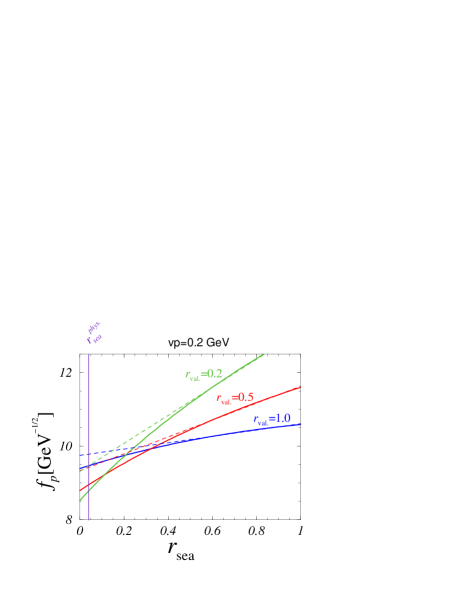
Figure 3: Comparison of complete $f_{p}^{B\to\pi}$ expressions in the partially quenched ${N_{\rm sea}}=2$ theory and the linear extrapolations. Here $v\negmedspace\cdot\negmedspace p=0.2$ GeV and ${r_{\rm val.}}=0.2,0.5,1.0$ are held fixed, while ${r_{\rm sea}}$ is varied. Linear fit is made to the PQChPT expressions from Appendix B in the range ${r_{\rm sea}}\in[0.5,1.0]$, and then extrapolated to the chiral limit. The vertical line marks the physical value ${r_{\rm sea}}=1/25$.

To examine the chiral behavior of the form factors we will use

$${r_{\rm val.}}={m_{\rm val.}}/m_{s}^{\text{phys}},\qquad{r_{\rm sea}}={m_{\rm sea}}/m_{s}^{\text{phys}}~{},$$ (40)

dimensionless parameters defined with respect to the physical strange quark mass. In the lattice studies, lowering the sea quark mass, ${m_{\rm sea}}$ (i.e., ${r_{\rm sea}}$), is numerically costlier than lowering the valence quark mass, ${m_{\rm val.}}$ (i.e., ${r_{\rm val.}}$). Fortunately, as discussed in the previous section, the dependence of $f_{p,v}(v\negmedspace\cdot\negmedspace p)$ on ${r_{\rm sea}}$ is expected to be linear, so that even larger extrapolations in ${m_{\rm sea}}$ may still lead to reasonably small extrapolation errors. This is illustrated in Fig. 3 for the case of the form factor $f_{p}$, with $v\negmedspace\cdot\negmedspace p=0.2$ GeV. We see that for small ${r_{\rm sea}}<{r_{\rm val.}}$ and ${r_{\rm sea}}\to 0$, the form factor is indeed a linear function of ${r_{\rm sea}}$, as already stated in Eq. (37). That behavior gets modified when ${r_{\rm sea}}>{r_{\rm val.}}$, resulting in the smooth forms that are very close to linear. If we linearly extrapolate the behavior of the form factors from the range of sea quark mass ${r_{\rm sea}}\in[0.5,1]$ down to the chiral limit, we observe only a small discrepancy with respect to the complete expression for $f_{p}$ (of about $5$ %). The same observation holds for the form factor $f_{v}$, with the discrepancy between the extrapolated and the result of the complete expression being approximately halved with respect to the one estimated for $f_{p}$. As it can be observed from Fig. 3, the uncertainty induced by the extrapolation in ${m_{\rm sea}}$ gets larger as the valence quark mass is decreased. However, for the quark masses that are realistic in the current lattice studies, ${r_{\rm val.}}\gtrsim 0.5$, the mentioned uncertainty is below the $5~{}\%$ level.

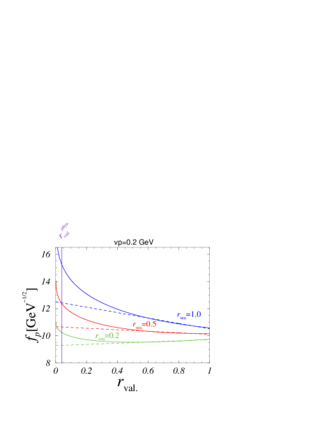
Figure 4: The situation similar to what is plotted in Fig. 3, but with ${r_{\rm sea}}$ and ${r_{\rm val.}}$ exchanging the roles, i.e., ${r_{\rm val.}}$ is varied for three fixed values of ${r_{\rm sea}}=0.2,0.5,1.0$.

The other possibility, i.e., to extrapolate $f_{p,v}$ in ${r_{\rm val.}}$ for a fixed value of ${r_{\rm sea}}$, is illustrated in Fig. 4. We see that in this case the difference between the linear extrapolation and the complete expression is much more pronounced, which reflects the presence of the quenched chiral logarithm $\propto{r_{\rm sea}}\ln({r_{\rm val.}})$, and hence the effect is larger for the heavier sea quark masses (cf. Eq. ((2))). Similar observations to the ones shown in Figs. 3 and 4, are also valid for the form factor $f_{v}$.

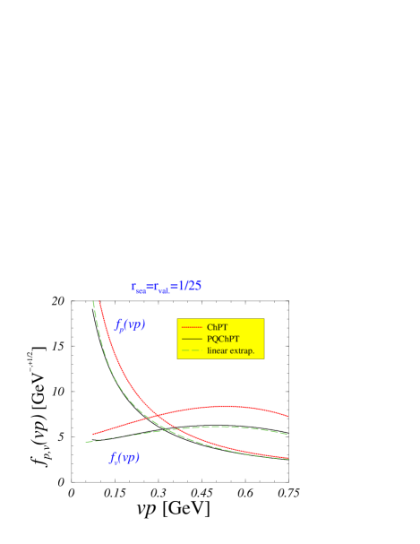
Figure 5: Solid lines show $f_{p,v}^{B\to\pi}(v\negmedspace\cdot\negmedspace p)$ in the partially quenched theory with ${N_{\rm sea}}=2$ at physical point ${r_{\rm sea}}={r_{\rm val.}}=1/25$. The dashed lines are obtained by first linearly extrapolating in ${r_{\rm sea}}$ then in ${r_{\rm val.}}$ to the physical point, as explained in the text. For an easier comparison we also plot the same form factors obtained in ChPT with $N=3$ by a dotted line (using the same values for low energy constants as in PQChPT with ${N_{\rm sea}}=2$).

An interesting observation is that the dependence of $f_{p,v}$ on ${r_{\rm val.}}$ (with ${r_{\rm sea}}$ and $v\negmedspace\cdot\negmedspace p$ fixed) is such that the form factors at the physical point ${r_{\rm val.}}\simeq 1/25$ are larger than what one gets from the linear extrapolation. On the other hand, when ${r_{\rm val.}}$ and $v\negmedspace\cdot\negmedspace p$ are fixed, the form factors at the physical point ${r_{\rm sea}}\simeq 1/25$ are smaller than the linearly extrapolated ones.

Therefore by first performing a linear extrapolation in ${r_{\rm sea}}$, and then in ${r_{\rm val.}}$ will not only allow one to avoid the spurious quenched logarithms, but it will also produce a mutual cancellation of the errors induced by the two chiral extrapolations. Indeed, the errors of the two consecutive extrapolations, as shown on Fig. 5, are strikingly small. Performing linear fits to the ${N_{\rm sea}}=2$ PQChPT expressions for ${r_{\rm sea}},{r_{\rm val.}}\in[0.5,1]$ leads to the errors below $5\%$, for both $f_{p}(v\negmedspace\cdot\negmedspace p)$ and $f_{v}(v\negmedspace\cdot\negmedspace p)$ form factors, and for a large range of $v\negmedspace\cdot\negmedspace p\in[0.05,0.75]$ GeV. If, however, the chiral extrapolation is made linearly by keeping the valence and sea quark masses equal, ${r_{\rm val.}}={r_{\rm sea}}$, the resulting error is in the $20\%$ range due to the explicit chiral logarithmic corrections given in Eq. ((3)).

For the reader’s convenience, in Fig. 5, we also plot the result of the fully unquenched theory with $N=3$. We observe a pleasant feature that the shapes of the form factors in these two theories are very similar. Notice also that the results obtained in PQChPT with ${N_{\rm sea}}=2$ are systematically lower from the ones obtained with ChPT $N=3$ by $10\%-20$%. It should be stressed, however, that this discrepancy might be artificial and merely a consequence of our assumption that the low energy constants do not change significantly when $N=2\to 3$. More information on the low energy constants in the theory with $N=2$ is needed to get a clearer picture on the significance of the differences depicted in Fig. 5.

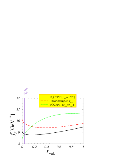
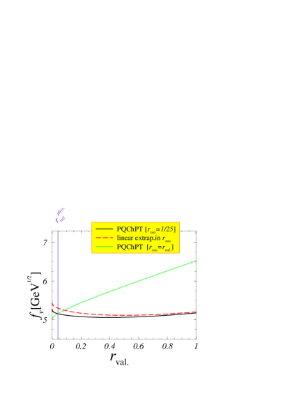
Figure 6: Solid lines show the ${r_{\rm val.}}$ dependence of $f_{p,v}^{B\to\pi}$ [Eq. (29)] in the partially quenched theory with ${N_{\rm sea}}=2$ and at ${r_{\rm sea}}=1/25$, $v\negmedspace\cdot\negmedspace p=0.2\ {\rm GeV}$. The dashed lines show the form factors linearly extrapolated from ${r_{\rm sea}}\in[0.5,1.0]$ down to physical point ${r_{\rm sea}}=1/25$. The dotted lines refer to the dependence on ${r_{\rm val.}}$ while keeping ${r_{\rm sea}}={r_{\rm val.}}$.

Another lesson comes from Fig. 6, where we plot the ${r_{\rm val.}}$ dependence of the form factors by using the complete ${N_{\rm sea}}=2$ expressions, derived in PQChPT, and by linearly extrapolating in ${r_{\rm sea}}$ as discussed above. We see that the error due to the use of linear extrapolation of $f_{p}$ in ${r_{\rm sea}}$ is fairly small at large ${r_{\rm val.}}$, but then increases as ${r_{\rm val.}}$ approaches its physical value. Reducing ${r_{\rm val.}}$ below ${r_{\rm val.}}<0.5$ in future lattice studies will therefore improve on the simple consecutive linear extrapolations (first in ${r_{\rm sea}}$, then in ${r_{\rm val.}}$, for ${r_{\rm sea}},{r_{\rm val.}}\in[0,5,1.0]$) only if, together with smaller ${r_{\rm val.}}$, also the smaller values of ${r_{\rm sea}}$ are reached in the simulation. For the high precision studies with both ${r_{\rm sea}}$ and ${r_{\rm val.}}$ well below $0.5$, it might even be more advantageous to use extrapolations with ${r_{\rm sea}}={r_{\rm val.}}$ (cf. Fig. 6, left), contrary to what we advocated for more realistic studies (at present), namely with ${r_{\rm sea}},{r_{\rm val.}}\gtrsim 0.5$.

Finally, we consider the soft pion theorem, which states that the ratio $F_{0}/(f_{B}/f_{\pi})\to 1$ as $v\negmedspace\cdot\negmedspace p$ and quark masses go to zero in full ChPT. We verified that this is satisfied also in partially quenched theory in the limit in which $v\negmedspace\cdot\negmedspace p\to 0$, and ${m_{\rm sea}}={m_{\rm val.}}\to 0$. Numerically, the ratio stays within $0.95<[F_{0}/(f_{B}/f_{\pi})]<1.25$ in the ranges of $v\negmedspace\cdot\negmedspace p<0.2~{}{\rm GeV}$ and $0<{r_{\rm val.}},{r_{\rm sea}}<1$, but it diverges for ${m_{\rm val.}}\to 0$ if ${m_{\rm sea}}\neq{m_{\rm val.}}$.

IV.2 Ratios $f_{p,v}^{B\to K}/f_{p,v}^{B\to\pi}$

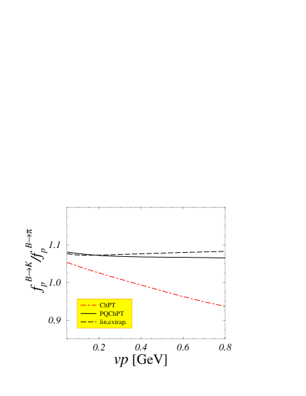
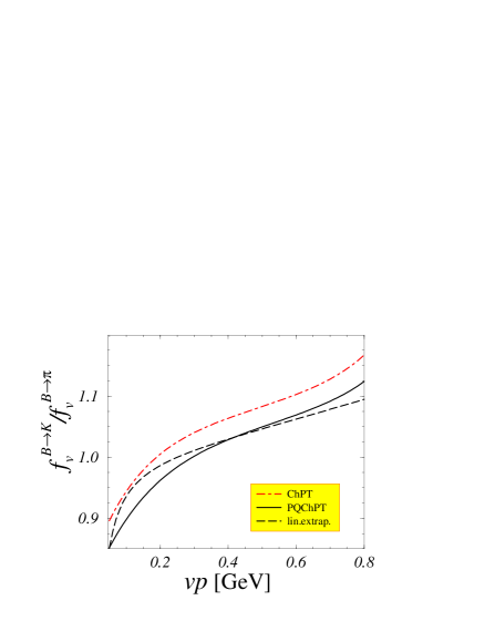
Figure 7: Behavior of the SU(3) breaking ratio $R_{p,v}=f_{p,v}^{B\to K}/f_{p,v}^{B\to\pi}$ (at physical values of quark masses) as functions of $v\cdot p$. The prediction of PQChPT with ${N_{\rm sea}}=2$ is denoted by the solid lines. The dashed curves are obtained after consecutive extrapolations, first in ${r_{\rm sea}}$ and then in ${r_{\rm val.}}$ (as explained in the text), while the dot-dashed curve is the prediction of the full ChPT with $N=3$.

Instead of repeating the previous discussion for the $B\to K$ form factors, we investigate the ratios $R_{p,v}=f_{p,v}^{B\to K}/f_{p,v}^{B\to\pi}$. Our kaon is composed of valence quarks with one mass fixed at the physical strange quark mass and the other varied, i.e., $M_{K}^{2}=2\mu_{0}m_{s}^{\text{phys}}(1+{r_{\rm val.}})$, whereas the pion valence content reads, $M_{\pi}^{2}=4\mu_{0}m_{s}^{\text{phys}}{r_{\rm val.}}$. We also ignore the difference between the poles in $f^{B\to K}_{p}$ and in $f^{B\to\pi}_{p}$, i.e., we take $m_{B^{\ast}}=m_{B_{s}^{\ast}}$.

We again observe the linear dependence of the ratio $R_{p,v}$ under varying the light sea quark mass, ${m_{\rm sea}}$, while keeping fixed values of ${m_{\rm val.}}$ and $v\negmedspace\cdot\negmedspace p$. As in the previous section we see that the variation of ${m_{\rm val.}}$ in the chiral limit at fixed ${m_{\rm sea}}$ exhibits both standard and quenched chiral logarithmic dependences. Therefore, like in the $B\to\pi$ case, a consecutive linear extrapolation in ${r_{\rm sea}}$ and then in ${r_{\rm val.}}$ leads to very small errors of extrapolation, namely below 5% (see Fig. 7).

In Fig. 7 we observe that the dependence of $R_{p}$ on $v\negmedspace\cdot\negmedspace p$, as inferred from the PQChPT with ${N_{\rm sea}}=2$, differs from the one obtained in the full ChPT with $N=3$ at the $10\%$ level. Note that this feature does not change under the variation of ${\cal O}(p^{3})$, ${\cal O}(p^{4})$ low energy constants given in Eqs. (22) and (10). In addition, the $v\negmedspace\cdot\negmedspace p$ dependence of $R_{p}$ in partially quenched theory does not change significantly when varying ${r_{\rm sea}}$ in the range ${r_{\rm sea}}\in(0,1)$. It is important to stress that the apparent disagreement between $R_{p}^{\rm PQChPT}$ and $R_{p}^{\rm ChPT}$ as functions of $v\negmedspace\cdot\negmedspace p$ disappears after replacing ${N_{\rm sea}}=2$ by ${N_{\rm sea}}=3$ in our PQChPT expressions. Finally, it should be mentioned that the absolute values of $R_{p,v}$ (but not their $v\negmedspace\cdot\negmedspace p$ behavior) may be further affected by the uncertainties in $\varkappa_{1}$ and $L_{5}$, because these constants enter the expressions for $R_{p,v}$, multiplied by $m_{K}^{2}$.

V Conclusions

In this paper we presented the expressions for the $heavy\to light$ pseudoscalar meson form factors as derived at NLO in PQChPT and in the static limit of HQET. This calculation is useful in the perspective of the QCD simulations on the lattice, since the most wanted $B\to\pi$ transition form factors are expected to be computed quite soon in the partially quenched QCD with ${N_{\rm sea}}=2$. The approach adopted in this paper is valid for small recoils (i.e., close to $q^{2}\to q^{2}_{\rm max}$), the part of the phase space that is also accessible by the current lattice simulations. The main benefit of the expressions derived in PQChPT lies in the fact that one can disentangle the chiral behavior in the sea quark mass, ${m_{\rm sea}}$, from the chiral dependence in the valence light quark mass, ${m_{\rm val.}}$. Our results clearly suggest a linear behavior of the form factors under the variation of the sea quark mass value ${m_{\rm sea}}$, when the valence quark mass ${m_{\rm val.}}$ is kept fixed. On the other hand, if the sea quark mass ${m_{\rm sea}}$ is fixed to some value that is directly accessible from the current lattice studies with ${N_{\rm sea}}=2$ (e.g. ${r_{\rm sea}}\gtrsim 0.5$), the form factors exhibit both the standard and quenched chiral logarithms when approaching the physical point, ${r_{\rm val.}}\simeq 1/25$. For that reason, we propose a strategy of computing the $B\to\pi(K)$ semileptonic form factors on the lattice (in partially quenched theory with ${N_{\rm sea}}=2$ degenerate light quarks) that requires a computation to be performed at several values of the sea quark mass with the valence quark mass held fixed. The extrapolation of $F_{+,0}(q^{2})$ in the sea quark mass to the physical $u$/$d$ quarks can then be made linearly at fixed valence quark mass. This should then be followed by an extrapolation in the valence quark mass. In this way the quenched logarithm is avoided since the pathological term is of the form ${m_{\rm sea}}\ln({m_{\rm val.}})$. As a result, the above procedure leads to results which are different by no more than $5\%$ with respect to the complete prediction of PQChPT with ${N_{\rm sea}}=2$. This makes a strong call for the partially quenched lattice computations of the $heavy\to light$ transition matrix elements with ${N_{\rm sea}}=2$.

Regarding the comparison of the form factors obtained in PQChPT with ${N_{\rm sea}}=2$ and the ones obtained in ChPT with $N=3$, we notice that the results obtained with $N=2$ are systematically lower than their $N=3$ counterparts. The difference is in the ball park of $10\%-20\%$. At this point it is not clear whether this difference is a realistic estimate of the present approach, or merely a consequence of our lack of knowledge of the values of the low energy constant in the theory with $N=2$. The above estimate of $10\%-20$% is obtained by assuming the low energy constants to be independent of the number of flavors.

Appendix A Chiral loop integrals

In this appendix we list the dimensionally regularized integrals encountered in the course of calculation. For more details, see Ref. jure, and references therein.

$$i\mu^{\epsilon}\int\frac{d^{4-\epsilon}q}{(2\pi)^{4-\epsilon}}\frac{1}{q^{2}-m^{2}} =\frac{1}{16\pi^{2}}I_{1}(m)\;,$$

$$i\mu^{\epsilon}\int\frac{d^{4-\epsilon}q}{(2\pi)^{4-\epsilon}}\frac{1}{(q^{2}-m^{2})(q\negmedspace\cdot\negmedspace v-\Delta)} =\frac{1}{16\pi^{2}}\frac{1}{\Delta}I_{2}(m,\Delta)\;,$$ (41)

where

$$I_{1}(m) =m^{2}\ln\Bigl{(}\frac{m^{2}}{\mu^{2}}\Bigr{)}-m^{2}\bar{\Delta}\;,$$

$$I_{2}(m,\Delta) =-2\Delta^{2}\ln\Bigl{(}\frac{m^{2}}{\mu^{2}}\Bigr{)}-4\Delta^{2}F\Bigl{(}\frac{m}{\Delta}\Bigr{)}+2\Delta^{2}(1+\bar{\Delta})\;,$$ (42)

where $\bar{\Delta}=2/\epsilon-\gamma+\ln(4\pi)+1$. The function $F(x)$ has been calculated in Ref. stewart, , for both the negative and positive values of the argument:

$$F\left(\frac{1}{x}\right)=\left\{\begin{aligned} -\frac{\sqrt{1-x^{2}}}{x}&\left[\frac{\pi}{2}-\tan^{-1}\left(\frac{x}{\sqrt{1-x^{2}}}\right)\right],\,&|x|\leq 1\\ \frac{\sqrt{x^{2}-1}}{x}&\ln\left(x+\sqrt{x^{2}-1}\right),\,&|x|\geq 1\;.\end{aligned}\right.$$ (43)

In addition to the integrals (A), one also needs the following two:

$$i\mu^{\epsilon}\int\frac{d^{4-\epsilon}q}{(2\pi)^{4-\epsilon}}\frac{q^{\mu}}{(q^{2}-m^{2})(q\negmedspace\cdot\negmedspace v-\Delta)}$$

$$=\frac{v^{\mu}}{16\pi^{2}}\left[I_{2}(m,\Delta)+I_{1}(m)\right]\;,$$ (44)

$$i\mu^{\epsilon}\int\frac{d^{4-\epsilon}q}{(2\pi)^{4-\epsilon}}\frac{q^{\mu}q^{\nu}}{(q^{2}-m^{2})(q\negmedspace\cdot\negmedspace v-\Delta)}$$

$$=\frac{1}{16\pi^{2}}\Delta\left[J_{1}(m,\Delta)\eta^{\mu\nu}+J_{2}(m,\Delta)v^{\mu}v^{\nu}\right]\;,$$ (45)

with

$$\begin{split}J_{1}(m,\Delta)=&(-m^{2}+\frac{2}{3}\Delta^{2})\ln\left(\frac{m^{2}}{\mu^{2}}\right)+\frac{4}{3}(\Delta^{2}-m^{2})F\left(\frac{m}{\Delta}\right)\\ &-\frac{2}{3}\Delta^{2}(1+\bar{\Delta})+\frac{1}{3}m^{2}(2+3\bar{\Delta})+\frac{2}{3}m^{2}-\frac{4}{9}\Delta^{2}\;,\end{split}$$ (46a)

$$\begin{split}J_{2}(m,\Delta)=&(2m^{2}-\frac{8}{3}\Delta^{2})\ln\left(\frac{m^{2}}{\mu^{2}}\right)-\frac{4}{3}(4\Delta^{2}-m^{2})F\left(\frac{m}{\Delta}\right)\\ &+\frac{8}{3}\Delta^{2}(1+\bar{\Delta})-\frac{2}{3}m^{2}(1+3\bar{\Delta})-\frac{2}{3}m^{2}+\frac{4}{9}\Delta^{2}\;.\end{split}$$ (46b)

The functions $J_{1}(m,\Delta),J_{2}(m,\Delta)$ differ from the ones in Ref. boyd, by the last two terms in Eq. (46) which are of ${\cal O}(m^{2},\Delta^{2})$. These additional (finite) terms originate from the fact that $\eta^{\mu\nu}$ is the ($4-\epsilon$)-dimensional metric tensor.

Appendix B Loop contributions to form factors in PQChPT

In this appendix we list expressions for the one-loop chiral corrections to the form factors $f_{p,v}$ [Eq. (36)] in partially quenched ChPT (the form factors for fully quenched ChPT and full ChPT are collected in Appendix B of Ref. JSD, ). The formulas apply to the $B_{a}\to P_{ba}$ transition with $B_{a}\sim b\bar{q}_{a}$ and $P_{ba}\sim q_{b}\bar{q}_{a}$. They are expressed in terms of the pseudoscalar meson masses $M_{a,b,S}^{2}=4\mu_{0}m_{a,b,{\rm sea}}$, $M_{ab}^{2}=2\mu_{0}(m_{a}+m_{b})$, and $M_{aS,bS}^{2}=2\mu_{0}(m_{a,b}+{m_{\rm sea}})$. We list the nonzero contributions to $f_{p,v}^{(I)}$, with the superscript “$I$” corresponding to a label of the diagram shown in Fig. 2.

$$\delta f_{p}^{(7)} = \frac{3g^{2}}{(4\pi f)^{2}}\ \Big{\{}{N_{\rm sea}}\left[J_{1}(M_{bS},v\negmedspace\cdot\negmedspace p)-\frac{1}{v\negmedspace\cdot\negmedspace p}\frac{2\pi}{3}M_{bS}^{3}\right]-\frac{1}{{N_{\rm sea}}}\left(1+\left(M_{b}^{2}-M_{S}^{2}\right)\frac{\partial}{\partial M_{b}^{2}}\right)\left[J_{1}(M_{b},v\negmedspace\cdot\negmedspace p)-\frac{1}{v\negmedspace\cdot\negmedspace p}\frac{2\pi}{3}M_{b}^{3}\right]\;,$$

$$\delta f_{p}^{(9)} = -\frac{g^{2}}{(4\pi f)^{2}}\frac{1}{{N_{\rm sea}}}\frac{1}{(M_{a}^{2}-M_{b}^{2})}\bigg{[}\left(M_{a}^{2}-M_{S}^{2}\right)\left(J_{1}(M_{a},v\negmedspace\cdot\negmedspace p)-\frac{1}{v\negmedspace\cdot\negmedspace p}\frac{2\pi}{3}M_{a}^{3}\right)-\left(M_{b}^{2}-M_{S}^{2}\right)\left(J_{1}(M_{b},v\negmedspace\cdot\negmedspace p)-\frac{1}{v\negmedspace\cdot\negmedspace p}\frac{2\pi}{3}M_{b}^{3}\right)\bigg{]}\;,$$

$$\delta f_{p}^{(12)} = -\frac{1}{6(4\pi f)^{2}}\biggl{\{}{N_{\rm sea}}\Big{(}I_{1}(M_{aS})+I_{1}(M_{bS})\Big{)}-\frac{1}{{N_{\rm sea}}}\Big{(}G_{1}(M_{a},M_{S})+G_{1}(M_{b},M_{S})\Big{)}\biggr{.}+\frac{2}{{N_{\rm sea}}}H_{1}(M_{a},M_{b},M_{S})\biggr{\}}\;,$$

$$\delta f_{p}^{(13)} = -\frac{1}{2(4\pi f)^{2}}\Big{[}{N_{\rm sea}}I_{1}(M_{bS})-\frac{1}{{N_{\rm sea}}}G_{1}(M_{b},M_{S})\Big{]}\,,$$ (47)

and

$$\delta f_{v}^{(4)} = \frac{1}{2(4\pi f)^{2}}\biggl{\{}{N_{\rm sea}}\Big{[}I_{1}(M_{bS})+2I_{2}(M_{bS},v\negmedspace\cdot\negmedspace p)\Big{]}+\frac{1}{{N_{\rm sea}}}\Big{[}H_{1}(M_{a},M_{b},M_{S})-G_{1}(M_{b},M_{S})\Big{]}$$

$$\hskip 180.67517pt+\frac{2}{{N_{\rm sea}}}\Big{[}H_{2}(M_{a},M_{b},M_{S},v\negmedspace\cdot\negmedspace p)-G_{2}(M_{b},M_{S},v\negmedspace\cdot\negmedspace p)\Big{]}\biggr{\}}\,,$$

$$\delta f_{v}^{(14)} = -\frac{1}{6(4\pi f)^{2}}\biggl{\{}{N_{\rm sea}}\Big{[}I_{1}(M_{aS})+I_{1}(M_{bS})\Big{]}-\frac{1}{{N_{\rm sea}}}\Big{[}G_{1}(M_{a},M_{S})+G_{1}(M_{b},M_{S})\Big{]}-\frac{1}{{N_{\rm sea}}}H_{1}(M_{a},M_{b},M_{S})\biggr{\}}~{}.$$

The one loop chiral corrections to the wave function renormalization factors $Z_{B,P}$ are

$$\delta Z_{P_{ab}}^{\text{Loop}} = \frac{1}{3(4\pi f)^{2}}\biggr{\{}{N_{\rm sea}}\Big{[}I_{1}(M_{aS})+I_{1}(M_{bS})\Big{]}+\frac{2}{{N_{\rm sea}}}H_{1}(M_{a},M_{b},M_{S})-\frac{1}{{N_{\rm sea}}}\Big{[}G_{1}(M_{a},M_{S})+G_{1}(M_{b},M_{S})\Big{]}\biggr{\}}\,,$$

$$\delta Z_{B_{a}}^{\text{Loop}} = \frac{3g^{2}}{(4\pi f)^{2}}\biggr{\{}-{N_{\rm sea}}I_{1}(M_{aS})+\frac{1}{{N_{\rm sea}}}G_{1}(M_{a},M_{S})\biggr{\}}~{}.$$ (49)

The functions $I_{1}(m)$, $I_{2}(m)$, and $J_{1}(m,\Delta)$ are given in Appendix A. In addition, we have used the abbreviations

$$G_{1}(M,M_{S}) =\frac{\partial}{\partial M^{2}}\left[(M^{2}-M_{S}^{2})I_{1}(M)\right]\,,$$ (50)

$$H_{1}(M_{a},M_{b},M_{S}) =\frac{1}{M_{a}^{2}-M_{b}^{2}}\left[\left(M_{a}^{2}-M_{S}^{2}\right)I_{1}(M_{a})\right.$$

$$-\left.\left(M_{b}^{2}-M_{S}^{2}\right)I_{1}(M_{b})\right]\,,$$ (51)

and similarly for $G_{2}(M,M_{S},v\negmedspace\cdot\negmedspace p)$ and $H_{2}(M_{a},M_{b},M_{S},v\negmedspace\cdot\negmedspace p)$, that are obtained by simply replacing $I_{1}(M)\to I_{2}(M,v\negmedspace\cdot\negmedspace p)$ in the above expressions. Note that in the limit of degenerate valence quarks, $M_{a}\to M_{b}$, we have

$$\lim_{M_{a}\to M_{b}}H_{1}(M_{a},M_{b},M_{S}) =G_{1}(M_{a},M_{S})\,,$$ (52)

$$\lim_{M_{a}\to M_{b}}H_{2}(M_{a},M_{b},M_{S},v\negmedspace\cdot\negmedspace p) =G_{2}(M_{a},M_{S},v\negmedspace\cdot\negmedspace p)\,.$$ (53)

We reiterate that the mass differences ($\Delta$) among $B$, $B^{\ast}$, $B_{s}$, and $B_{s}^{\ast}$ mesons have been consistently neglected in the loops, since $v\negmedspace\cdot\negmedspace p>\Delta^{\ast}$, for the $B\to\pi,K$ transitions. This induces a spurious singularity in the expression for the diagrams (7), at $v\negmedspace\cdot\negmedspace p\to 0$. To handle such singularities we followed the proposal by Falk and Grinstein falk and resum the corresponding diagrams and then simply subtract the term that would renormalize the $B^{\ast}$-meson mass.

References

• (1) UKQCD Collaboration, K. C. Bowler et al., Phys. Lett. B 486, 111 (2000); APE Collaboration, A. Abada et al., Nucl. Phys. B 619, 565 (2001); JLQCD Collaboration, S. Aoki et al., Phys. Rev. D 64, 114505 (2001); A. X. El-Khadra et al., ibid 64, 014502 (2001); J. Shigemitsu et al., ibid 66, 074506 (2002).
• (2) S. R. Sharpe, Phys. Rev. D 46, 3146 (1992).
• (3) C. W. Bernard and M. F. Golterman, Phys. Rev. D 46, 853 (1992).
• (4) A. Morel, J. Phys. (France) 48, 1111 (1987).
• (5) M. J. Booth, Phys. Rev. D 51, 2338 (1995).
• (6) S. R. Sharpe and Y. Zhang, Phys. Rev. D 53, 5125 (1996).
• (7) D. Becirevic, S. Prelovsek, and J. Zupan, Phys. Rev. D 67, 054010 (2003).
• (8) C. W. Bernard and M. F. Golterman, Phys. Rev. D 49, 486 (1994)
• (9) P. H. Damgaard, J. C. Osborn, D. Toublan, and J. J. Verbaarschot, Nucl. Phys. B 547, 305 (1999).
• (10) S. R. Sharpe and N. Shoresh, Phys. Rev. D 64, 114510 (2001); 62, 094503 (2000).
• (11) J. Gasser and H. Leutwyler, Nucl. Phys. B 250, 465 (1985).
• (12) J. F. Donoghue, E. Golowich, and B. R. Holstein, “Dynamics Of The Standard Model”, Cambridge Monogr. Part. Phys. Nucl. Phys. Cosmol.  2, 1 (1992).
• (13) R. Casalbuoni, A. Deandrea, N. Di Bartolomeo, R. Gatto, F. Feruglio, and G. Nardulli, Phys. Rep.  281, 145 (1997); B. Grinstein, hep-ph/9508227; A. V. Manohar and M. B. Wise, “Heavy Quark Physics”, Cambridge Monogr. Part. Phys. Nucl. Phys. Cosmol.  10, 1 (2000).
• (14) G. Burdman and J. F. Donoghue, Phys. Lett. B 280, 287 (1992); M. B. Wise, Phys. Rev. D 45, 2188 (1992); J. L. Goity, Phys. Rev. D 46, 3929 (1992).
• (15) H. Leutwyler, “Chiral dynamics”, hep-ph/0008124; A. Pich, Rep. Prog. Phys.  58, 563 (1995); G. Ecker, “Strong interactions of light flavours”, hep-ph/0011026; U. G. Meissner, Rep. Prog. Phys.  56, 903 (1993); G. Colangelo, G. Isidori, “An introduction to ChPT”, hep-ph/0101264.
• (16) E. Eichten and B. Hill, Phys. Lett. B 234, 511 (1990); D. J. Broadhurst and A. G. Grozin, Phys. Rev. D 52, 4082 (1995).
• (17) N. Isgur and M. B. Wise, Phys. Rev. D 42, 2388 (1990).
• (18) D. Becirevic, S. Fajfer, S. Prelovsek, and J. Zupan, Phys. Lett. B 563, 150 (2003).
• (19) JLQCD Collaboration, S. Aoki et al., Phys. Rev. D 68, 054502 (2003); H. Wittig, hep-lat/0210025.
• (20) J. Zupan, Eur. Phys. J. C 25, 233 (2002); A. O. Bouzas, ibid 12, 643 (2000).
• (21) I. W. Stewart, Nucl. Phys. B 529, 62 (1998).
• (22) C. G. Boyd and B. Grinstein, Nucl. Phys. B 442, 205 (1995).
• (23) A. F. Falk and B. Grinstein, Nucl. Phys. B 416, 771 (1994).