SU($N$) Glueball Masses in 2+1 Dimensions

Abstract

We calculate the masses of the lowest lying eigenstates of improved SU(2), SU(3), SU(4) and SU(5) Hamiltonian lattice gauge theory (LGT) in 2+1 dimensions using an analytic variational approach. The ground state is approximated by a one plaquette trial state and mass gaps are calculated in the symmetric and antisymmetric sectors by minimising over a suitable basis of rectangular states. Analytic techniques are developed to handle the group integrals arising in the calculation.

I Introduction

In this paper we calculate the lowest lying glueball masses for SU($N$) LGT in 2+1 dimensions, with $N=2$, 3, 4 and 5, extending an earlier paper which considered $N=2$ and 3 Carlsson et al. (2002). We use Kogut-Susskind Kogut and Susskind (1975), classically improved and tadpole improved Hamiltonians Carlsson and McKellar (2001) in their calculation and develop analytic techniques for the calculation of the required expectation values.

The outline of this paper is as follows. In Section II we develop analytic techniques for use in the calculation of certain group integrals for general SU($N$). When used as generating functions these integrals allow an analytic treatment of the matrix elements appearing in later sections. After defining our notation in Section III we fix the variational vacuum wave function in Section IV. Following that we calculate lattice specific heats in Section V before studying SU($N$) glueball masses in Section VI. Section VIII contains our conclusions and a discussion of further work.

II Analytic techniques for SU($N$)

II.1 The special cases of SU(2) and SU(3)

In this section we recall two results which are useful in the calculation of group integrals for the special cases of SU(2) and SU(3). For further details we refer the reader to Ref. Carlsson et al., 2002. Before presenting these results the concept of group integration needs to be introduced. For this purpose we introduce the one plaquette trial state, which we will use to simulate the ground, or (perturbed) vacuum, state with energy $E_{0}$,

$$\begin{array}[]{c}\includegraphics{thesis-paper1-eqn1.eps}\end{array}$$ (1)

Here, $|0\rangle$ is the strong coupling vacuum defined by ${\cal E}^{\alpha}_{i}(\bm{x})|0\rangle=0$ for all $i$, $\bm{x}$ and $\alpha=1,2,\ldots,N^{2}-1$. ${\cal E}^{\alpha}_{i}(\bm{x})$ is the lattice chromoelectric field on the directed link running from the lattice site labelled by $\bm{x}$ to the site labelled by $\bm{x}+a\bm{i}$. The directed square denotes the traced ordered product of link operators, $U_{i}(\bm{x})$, around an elementary square, or plaquette, of the lattice,

$$\begin{array}[]{c}\includegraphics{thesis-paper1-eqn2.eps}\end{array}$$ (2)

where $a$ is the lattice spacing. With this notation understood, we can write the expectation value of a plaquette as an SU($N$) group integral as follows

$$\begin{array}[]{c}\includegraphics{thesis-paper1-eqn3.eps}\end{array}$$ (3)

Here the products over $l$ and $l^{\prime}$ extend over all links on the lattice, while the products over $p$ and $p^{\prime}$ extend over all plaquettes on the lattice. In Eq. (3) we introduced the notation $Z_{1}(p)$ to denote the trace of plaquette $p$. For each integral in Eq. (3) the integration measure is given by the Haar measure (also called the invariant measure and less commonly the Hurwitz measure) Montvay and Münster (1994); Creutz (1983). For any compact group $G$, the Haar measure is the unique measure $dU$ on $G$ which is left and right invariant,

$$\int_{G}dUf(U)=\int_{G}dUf(VU)=\int_{G}dUf(UV)\hskip 28.45274pt\forall V\in G$$ (4)

and normalised,

$$\int_{G}dU=1.$$ (5)

In Eq. (4) $f$ is an arbitrary function over $G$.

In 2+1 dimensions the variables in Eq. (3) can be changed from links to plaquettes with unit Jacobian Batrouni and Halpern (1984). The plaquettes then become independent variables allowing the cancellation of all but one group integral in Eq. (3). All that remains is

$$\begin{array}[]{c}\includegraphics{thesis-paper1-eqn6.eps}\end{array}$$ (6)

Here, $V$ is a plaquette variable with ${\rm Tr}V=Z_{1}(0)$. For the case of SU(2), analytic expressions for the plaquette expectation value in terms of modified Bessel functions have been used in variational calculations for almost 20 years. A key result Arisue et al. (1983) is

$$\int_{{\rm SU}(2)}dUe^{c{\rm Tr}U}=\frac{1}{c}I_{1}(2c).$$ (7)

Here $I_{n}$ is the $n$-th order modified Bessel function of the first kind defined, for all integers $n$, by

$$I_{n}(2x)=\sum_{k=0}^{\infty}\frac{x^{2k+n}}{k!(k+n)!}.$$ (8)

In an earlier paper, we showed that the corresponding SU(3) result follows simply from a paper of Eriksson, Svartholm and Skagerstam Eriksson et al. (1981), with the result:

$$\int_{{\rm SU}(3)}dUe^{c{\rm Tr}U+d{\rm Tr}U^{\dagger}} = 2\sum_{k=0}^{\infty}\frac{1}{(k+1)!(k+2)!}\sum_{l=0}^{k}\left(\!\begin{array}[]{c}3k+3\\ k-l\end{array}\!\right)\frac{1}{l!}(cd)^{k-l}(c^{3}+d^{3})^{l}.$$ (11)

In the next section we derive the general SU($N$) result as well as a selection of other useful SU($N$) group integrals.

II.2 The generalisation to SU($N$)

II.2.1 Introduction

Much work has been carried out on the topic of integration over the classical compact groups. The subject has been studied in great depth in the context of random matrices and combinatorics. Many analytic results in terms of determinants are available for integrals of various functions over unitary, orthogonal and symplectic groups Baik and Rains (2001). Unfortunately similar results for SU($N$) are not to our knowledge available. Their primary use has been in the study of Ulam’s problem concerning the distribution of the length of the longest increasing subsequence in permutation groups Rains (1998); Widom et al. (2001). Connections between random permutations and Young tableaux Regev (1981) allow an interesting approach to combinatorial problems involving Young tableaux. A problem of particular interest is the counting of Young tableaux of bounded height Gessel (1990) which is closely related to the problem of counting singlets in product representations mentioned in Section II.1. Group integrals similar to those needed in this paper have also appeared in studies of the distributions of the eigenvalues of random matrices Diaconis and Shahshahani (1994); Widom and Tracy (1999).

In the context of LGT not much has work been done in the last 20 years on the subject of group integration. The last significant development was due to Creutz who developed a diagrammatic technique for calculating specific SU($N$) integrals Creutz (1978) using link variables. This technique allows strong coupling matrix elements to be calculated for SU($N$) Leonard (2001) and has more recently been used in the loop formulation of quantum gravity where spin networks are of interest De Pietri (1997); Rovelli and Smolin (1995); Ezawa (1997).

In Sections II.2.2 and II.2.3 we extend the results of Section II.1 to calculate two important SU($N$) integrals. As generating functions these integrals allow the evaluation of all expectation values appearing in variational calculations of SU($N$) glueball masses in 2+1 dimensions. To calculate these generating functions we work with plaquette variables and make use of techniques which have become standard practice in the fields of random matrices and combinatorics. In Section II.2.2 we derive a generating function which allows the calculation of integrals of the form

$$\int_{{\rm SU}(N)}dU({\rm Tr}U)^{m}\overline{({\rm Tr}U)}^{n}e^{c({\rm Tr}U+{\rm Tr}U^{\dagger})}.$$ (12)

The work in Section II.2.3 generalises the generating function of Section II.2.2 allowing the calculation of more complicated integrals of the form

$$\int_{{\rm SU}(N)}dU\left[{\rm Tr}(U^{l})\right]^{m}e^{c({\rm Tr}U+{\rm Tr}U^{\dagger})}.$$ (13)

For each integral considered the approach is the same and proceeds as follows. We start with a calculation of a U($N$) integral. For example in Section II.2.2 we calculate

$$G_{{\rm U}(N)}(c,d) = \int_{{\rm U}(N)}dUe^{c{\rm Tr}U+d{\rm Tr}U^{\dagger}}.$$ (14)

This is a generalisation of $G_{{\rm U}(N)}(c,c)$, an integral first calculated by Kogut, Snow and Stone Kogut et al. (1982). We then make use of a result of Brower, Rossi and Tan Brower et al. (1981) to extend the U($N$) integral to SU($N$) by building the restriction, $\det U=1$ for all $U\in$ SU($N$), into the integration measure. In this way SU($N$) generating functions can be obtained as sums of determinants whose entries are modified Bessel functions of the first kind.

II.2.2 A simple integral

In this section we introduce a useful technique for performing SU($N$) integrals. We start with the U($N$) integral of Eq. (14) and calculate it using a technique which has become standard practice in the study of random matrices and combinatorics.

Since the Haar measure is left and right invariant (see Eq. (4)) we can diagonalise $U$ inside the integral as

$$U=V\left(\begin{array}[]{cccc}e^{i\phi_{0}}&0&\cdots&0\\ 0&e^{i\phi_{1}}&&\vdots\\ \vdots&&\ddots&\\ 0&\cdots&&e^{i\phi_{N}}\end{array}\right)V^{\dagger}.$$ (19)

In terms of the set of variables $\{\phi_{k}\}_{k=1}^{N}$ the Haar measure factors as $dU=d\mu(\phi)dV$ Kogut et al. (1982). Since the integrand is independent of $V$, the $V$ integral can be carried out trivially using the normalisation of the Haar measure given by Eq. (5).

Making use of the Weyl parameterisation for U($N$) Weyl (1946),

$$d\mu(\phi) = \prod_{i=1}^{N}\frac{d\phi_{i}}{2\pi}|\Delta(\phi)|^{2},$$ (20)

where $\Delta(\phi)$ is the Vandermonde determinant, with implicit sums over repeated indices understood,

$$\Delta(\phi) = \frac{1}{\sqrt{N!}}\varepsilon_{i_{1}i_{2}\cdots i_{N}}e^{i\phi_{1}(N-i_{1})}e^{i\phi_{2}(N-i_{2})}\cdots e^{i\phi_{N}(N-i_{N})},$$ (21)

we can express the U($N$) generating function as follows

$$G_{{\rm U}(N)}(c,d) = \int_{0}^{2\pi}\frac{d\phi_{1}}{2\pi}\cdots\int_{0}^{2\pi}\frac{d\phi_{N}}{2\pi}\exp\left[\sum_{i=1}^{N}(ce^{i\phi_{i}}+de^{-i\phi_{i}})\right]|\Delta(\phi)|^{2}.$$ (22)

In Eq. (21), $\varepsilon_{i_{1}\ldots i_{n}}$ is the totally antisymmetric Levi-Civita tensor defined to be 1 if $\{i_{1},\ldots,i_{n}\}$ is an even permutation of $\{1,2,\ldots,n\}$, $-1$ if it is an odd permutation and 0 otherwise (i.e. if an index is repeated). Substituting Eq. (21) in Eq. (22) gives,

$$G_{{\rm U}(N)}(c,d) = \frac{1}{N!}\varepsilon_{i_{1}i_{2}\ldots i_{N}}\varepsilon_{j_{1}j_{2}\ldots j_{N}}\prod_{k=1}^{N}\int_{0}^{2\pi}\frac{d\phi_{k}}{2\pi}\exp\left[i(j_{k}-i_{k})\phi_{k}+ce^{i\phi_{k}}+de^{-i\phi_{k}}\right].$$ (23)

To simplify this further we need an expression for the integral,

$$g_{n}(c,d) = \int_{0}^{2\pi}\frac{dx}{2\pi}\exp(inx+ce^{ix}+de^{-ix}),$$ (24)

which is easily handled by expanding the integrand in Taylor series in $c$ and $d$,

$$g_{n}(c,d) = \sum_{k=0}^{\infty}\sum_{l=0}^{\infty}\frac{c^{k}d^{l}}{k!l!}\int\frac{dx}{2\pi}e^{ix\left(k-l+n\right)}$$ (25)

$$= \sum_{k=0}^{\infty}\frac{c^{k}d^{k+n}}{k!(k+n)!}$$

$$= \left(\frac{d}{c}\right)^{n/2}I_{n}\left(2\sqrt{cd}\right).$$

Making use of Eq. (25) in Eq. (23) gives an expression for $G_{{\rm U}(N)}(c,d)$ as a Toeplitz determinant (a determinant of a matrix whose $(i,j)$-th entry depends only on $j-i$),

$$G_{{\rm U}(N)}(c,d) = \frac{1}{N!}\varepsilon_{i_{1}i_{2}\ldots i_{N}}\varepsilon_{j_{1}j_{2}\ldots j_{N}}\prod_{k=1}^{N}g_{j_{k}-i_{k}}(c,d)$$ (26)

$$= \frac{1}{N!}\varepsilon_{i_{1}i_{2}\ldots i_{N}}\varepsilon_{j_{1}j_{2}\ldots j_{N}}\left(\frac{d}{c}\right)^{\sum_{l=0}^{N}(i_{l}-j_{l})/2}\prod_{k=1}^{N}I_{j_{k}-i_{k}}\left(2\sqrt{cd}\right)$$

$$= \det\left[I_{j-i}\left(2\sqrt{cd}\right)\right]_{1\leq i,j\leq N}.$$

Here the quantities inside the determinant are to be interpreted as the $(i,j)$-th entry of an $N\times N$ matrix. Now to calculate the corresponding SU($N$) result the restriction $\det U=1$, which is equivalent to $\sum_{k=1}^{N}\phi_{k}=0\,{\rm mod}\,2\pi$ in terms of the $\phi_{k}$ variables, must be built into the integration measure. To do this we follow Brower, Rossi and Tan Brower et al. (1981) and incorporate the following delta function in the integrand of Eq. (22):

$$2\pi\delta\left(\sum_{k=1}^{N}\phi_{k}-0\,{\rm mod}\,2\pi\right) = \sum_{m=-\infty}^{\infty}2\pi\delta\left(\sum_{k=1}^{N}\phi_{k}-2\pi m\right).$$ (27)

This is most conveniently introduced into the integral via its Fourier transform,

$$\sum_{m=-\infty}^{\infty}\exp\left(im\sum_{k=1}^{N}\phi_{k}\right).$$ (28)

To obtain the SU($N$) integral from the corresponding U($N$) result the modification is therefore trivial. Including Eq. (28) in the integrand of Eq. (22) leads to the general SU($N$) result,

$$G_{{\rm SU}(N)}(c,d) = \int_{{\rm SU}(N)}dUe^{c{\rm Tr}U+d{\rm Tr}U^{\dagger}}$$ (29)

$$= \sum_{m=-\infty}^{\infty}\det\left[g_{m+j-i}(c,d)\right]_{1\leq i,j\leq N}.$$

This expression can be manipulated to factor the $d/c$ dependence out of the determinant as follows,

$$\det\left[\left(\frac{d}{c}\right)^{(l+j-i)/2}I_{l+j-i}\left(2\sqrt{cd}\right)\right]_{1\leq i,j\leq N} = \frac{1}{N!}\varepsilon_{i_{1}i_{2}\ldots i_{N}}\varepsilon_{j_{1}j_{2}\ldots j_{N}}\left(\frac{d}{c}\right)^{lN/2+\sum_{k}(j_{k}-i_{k})/2}$$ (30)

$$\times\prod_{m=1}^{N}I_{l+j_{m}-i_{m}}\left(2\sqrt{cd}\right)$$

$$= \left(\frac{d}{c}\right)^{lN/2}\det\left[I_{l+j-i}\left(2\sqrt{cd}\right)\right]_{1\leq i,j\leq N}.$$

Making use of this result in Eq. (29) leads to the SU($N$) generating function

$$G_{{\rm SU}(N)}(c,d) = \sum_{l=-\infty}^{\infty}\left(\frac{d}{c}\right)^{lN/2}\det\left[I_{l+j-i}\left(2\sqrt{cd}\right)\right]_{i\leq i,j\leq N}.$$ (31)

For the case of SU(2) we can show that this reduces to the standard result of Arisue given by Eq. (7). To do this we need the recurrence relation for modified Bessel functions of the first kind,

$$I_{n-1}(x)-I_{n+1}(x)=\frac{2n}{x}I_{n}(x).$$ (32)

Recall that for SU(2) the Mandelstam constraint is ${\rm Tr}U={\rm Tr}U^{\dagger}$, so the case $G_{{\rm SU}(2)}(c,c)$ can be considered without loss of generality;

$$G_{{\rm SU}(2)}(c,c) = \sum_{l=-\infty}^{\infty}\left[I_{l}(2c)^{2}-I_{l-1}(2c)I_{l+1}(2c)\right]$$ (33)

$$= I_{0}(4c)-I_{2}(4c).$$

Here we have used the standard addition formula Gradshteyn and Ryzhik (1994) for modified Bessel functions. Employing the recurrence relation of Eq. (32) gives

$$G_{{\rm SU}(2)}(c,c) = \frac{1}{2c}I_{1}(4c),$$ (34)

which is the standard result of Arisue given by Eq. (7).

With an analytic form for SU($N$) in hand we can attempt to find simpler expressions for $G_{\rm{SU}(N)}(c,d)$ analogous to Eq. (34). To our knowledge no general formulas are available for the simplification of the determinants appearing in Eq. (31). Without such formulas we can resort to the crude method of analysing series expansions and comparing them with known expansions of closed form expressions. Since the determinants appearing in the generating function are nothing more than products of modified Bessel functions we expect that if a closed form expression for the general SU($N$) generating function exists, it will involve the generalised hypergeometric function. With this approach we have limited success. The SU(3) result of Eq. (11) is recovered numerically but the SU(4) result does simplify analytically.

When analysing the series expansion of $G_{\rm{SU}(4)}(c,c)$ we notice that it takes the form of a generalised hypergeometric function. In particular we find the following result:

$$G_{{\rm SU}(4)}(c,c) = {}_{2}F_{3}\left[\begin{array}[]{c}\frac{3}{2},\frac{5}{2}\\ 3,4,5\end{array};16c^{2}\right].$$ (37)

Here the generalised hypergeometric function is defined by

$${}_{p}F_{q}\left[\begin{array}[]{c}a_{1},a_{2},\ldots,a_{p}\\ b_{1},b_{2},\ldots,b_{q}\end{array};x\right]=\sum_{k=0}^{\infty}\frac{(a_{1})_{k}(a_{2})_{k}\ldots(a_{p})_{k}}{(b_{1})_{k}(b_{2})_{k}\ldots(b_{q})_{k}}\frac{x^{k}}{k!},$$ (40)

where $(x)_{k}=x(x+1)\ldots(x+k-1)$ is the rising factorial or Pochhammer symbol. In addition to Eq. (37) we find the following results for matrix elements derived from the SU(4) generating function:

$$\langle Z_{1}\rangle \!\!\!=\!\!\! \frac{c\,{}_{2}F_{3}\left[\!\begin{array}[]{c}\frac{5}{2},\frac{7}{2}\\ 4,5,6\end{array};16c^{2}\right]}{{}_{2}F_{3}\left[\!\begin{array}[]{c}\frac{3}{2},\frac{5}{2}\\ 3,4,5\end{array};16c^{2}\right]},$$ (45)

$$\langle Z_{1}^{2}\rangle \!\!\!=\!\!\! \frac{\frac{3}{2}c^{2}\,{}_{2}F_{3}\left[\!\begin{array}[]{c}\frac{5}{2},\frac{7}{2}\\ 5,6,7\end{array};16c^{2}\right]+\frac{2}{3}c^{4}\,{}_{2}F_{3}\left[\!\begin{array}[]{c}\frac{7}{2},\frac{9}{2}\\ 6,7,8\end{array};16c^{2}\right]+\frac{1}{15}c^{6}\,{}_{2}F_{3}\left[\!\begin{array}[]{c}\frac{9}{2},\frac{11}{2}\\ 7,8,9\end{array};16c^{2}\right]}{{}_{2}F_{3}\left[\!\begin{array}[]{c}\frac{3}{2},\frac{5}{2}\\ 3,4,5\end{array};16c^{2}\right]}$$ (54)

and

$$\langle Z_{1}\bar{Z}_{1}\rangle \!\!\!=\!\!\! \frac{{}_{2}F_{3}\left[\!\begin{array}[]{c}\frac{3}{2},\frac{5}{2}\\ 3,5,6\end{array};16c^{2}\right]+\frac{4}{3}c^{2}\,{}_{2}F_{3}\left[\!\begin{array}[]{c}\frac{5}{2},\frac{7}{2}\\ 4,6,7\end{array};16c^{2}\right]+\frac{4}{9}c^{4}\,{}_{2}F_{3}\left[\!\begin{array}[]{c}\frac{7}{2},\frac{9}{2}\\ 5,7,8\end{array};16c^{2}\right]}{{}_{2}F_{3}\left[\!\begin{array}[]{c}\frac{3}{2},\frac{5}{2}\\ 3,4,5\end{array};16c^{2}\right]}.$$ (63)

We stress that these results are nothing more than observations based on series expansions. Despite some effort analogous expressions for $N>4$ have not been found.

The generating functions, $G_{{\rm SU}(N)}(c,d)$ and $G_{{\rm U}(N)}(c,d)$, are not only of interest in Hamiltonian LGT. By differentiating Eq. (31) appropriately with respect to $c$ and $d$ and afterwards setting $c$ and $d$ to zero, we obtain the number of singlets in a given product representation of SU($N$). This was discussed for the special case of SU(3) in Section II.1. We now consider the general case in the calculation of $T_{k}(n)$; the number of singlets in the SU($k$) product representation,

$$\underbrace{({\bf k}\otimes{\bf\bar{k}})\otimes\cdots\otimes({\bf k}\otimes{\bf\bar{k}})}_{n}.$$ (64)

As a group integral $T_{k}(n)$ is given by

$$T_{k}(n)=\int_{{\rm SU}(k)}dU(|{\rm Tr}U|^{2})^{n}.$$ (65)

Integrals of this kind are studied in combinatorics, in particular the study of increasing subsequences of permutations. An increasing subsequence is a sequence $i_{1}<i_{2}<\cdots<i_{m}$ such that $\pi(i_{1})<\pi(i_{2})<\cdots<\pi(i_{m})$, where $\pi$ is a permutation of $\{1,2,\ldots,k\}$. It has been shown that the number of permutations $\pi$ of $\{1,2,\ldots,k\}$ such that $\pi$ has no increasing subsequence of length greater than $n$ is $T_{k}(n)$ Rains (1998). In addition it is possible to prove that $T_{k}(n)$ is the number of pairs of Young tableaux of size $k$ and maximum height $n$ via the Schensted correspondence van Moerbeke (2001); Rains (1998).

Making use of Eq. (31) we see that only the $l=0$ term contributes to $T_{k}(n)$. Letting $x=cd$ we have:

$$T_{k}(n) = (\partial_{c}\partial_{d})^{n}\det\left[I_{j-i}(2\sqrt{cd})\right]_{1\leq i,j\leq k}\Bigg{|}_{c=d=0}$$ (66)

$$= n!\frac{d^{n}}{dx^{n}}\det\left[I_{j-i}(2\sqrt{x})\right]_{1\leq i,j\leq k}\Bigg{|}_{x=0}.$$

Hence the generating function for $T_{k}(n)$ is given by

$$\sum_{n=0}^{\infty}\frac{T_{k}(n)x^{n}}{n!^{2}} = \det\left[I_{j-i}(2\sqrt{x})\right]_{1\leq i,j\leq k},$$ (67)

a result first deduced by Gessel Gessel (1990). The first few $T_{k}(n)$ sequences are available as A072131, A072132, A072133 and A072167 in Sloane’s on-line encyclopedia of integer sequences Sloane .

II.2.3 A more complicated integral

We now move on to the more complicated integral

$$H_{m}(c,d) = \int_{{\rm SU}(N)}dU\exp\left[c({\rm Tr}U+{\rm Tr}U^{\dagger})+d{\rm Tr}(U^{m})\right]\quad\forall m\in\mathbb{Z}^{+}.$$ (68)

This integral is of interest as a generating function for the calculation of integrals such as

$$\int_{{\rm SU}(N)}dU{\rm Tr}(U^{m})e^{c({\rm Tr}U+{\rm Tr}U^{\dagger})}.$$ (69)

For the simple case of SU(3) we can use the Mandelstam constraint, ${\rm Tr}(U^{2})=({\rm Tr}U)^{2}-2{\rm Tr}U^{\dagger}$, to reduce such integrals to those obtainable from $G_{{\rm SU}(N)}(c,d)$ . However for higher dimensional gauge groups not all trace variables can be written in terms of ${\rm Tr}U$ and ${\rm Tr}U^{\dagger}$. For these gauge groups one must introduce the generating function, $H_{m}(c,d)$, to calculate integrals similar to Eq. (69).

To calculate $H_{m}(c,d)$ we start with the corresponding U($N$) generating function $h_{m}(c,d)$ and follow the procedure of Section II.2.2 to obtain

$$h_{m}(c,d) = \int_{{\rm U}(N)}dU\exp\left[c({\rm Tr}U+{\rm Tr}U^{\dagger})+d{\rm Tr}(U^{m})\right]$$ (70)

$$=\frac{1}{N!}\varepsilon_{i_{1}\ldots i_{N}}\varepsilon_{j_{1}\ldots j_{N}}\prod_{k=1}^{N}\int_{0}^{2\pi}\frac{d\phi_{k}}{2\pi}\exp\left[i(j_{k}-i_{k})\phi_{k}+2c\cos\phi_{k}+de^{mi\phi_{k}}\right].$$

To proceed we need the following integral,

$$\int_{0}^{2\pi}\frac{dx}{2\pi}\exp(inx+a\cos x+be^{imx}) = \sum_{k=0}^{\infty}\frac{b^{k}}{k!}\int_{0}^{2\pi}\frac{dx}{2\pi}e^{i(n+mk)x+a\cos x}$$ (71)

$$= \sum_{k=0}^{\infty}\frac{b^{k}}{k!}I_{n+mk}(a).$$

Making use of Eq. (71) in Eq. (70) leads to the following expression for the U($N$) generating function,

$$h_{m}(c,d) = \det\left[\lambda_{m;j-i}(c,d)\right]_{1\leq i,j\leq N},$$ (72)

with

$$\lambda_{m;n}(c,d)=\sum_{k=0}^{\infty}\frac{d^{k}}{k!}I_{n+mk}(2c).$$ (73)

Extending to SU($N$) following the prescription of Section II.2.2, we arrive at the corresponding SU($N$) generating function,

$$H_{m}(c,d) = \sum_{l=-\infty}^{\infty}\det\left[\lambda_{m;l+j-i}(c,d)\right]_{1\leq i,j\leq N}.$$ (74)

An example of an SU($N$) integral derived from this generating function is the following:

$$\int_{{\rm SU}(N)}dU{\rm Tr}(U^{m})e^{c({\rm Tr}U+{\rm Tr}U^{\dagger})} = \frac{\partial H_{m}(c,d)}{\partial d}\Bigg{|}_{d=0}$$ (75)

$$= \frac{\partial}{\partial d}\sum_{l=-\infty}^{\infty}\det\left[I_{l+j-i}(2c)+dI_{l+j-i+m}(2c)\right]\Bigg{|}_{d=0}.$$

Only two terms need to be kept in the $k$-sum of Eq. (73) here because higher order powers of $d$ vanish when the derivative with respect to $d$ is taken and $d$ set to zero.

III Analytic SU($N$) Calculations

III.1 Preliminaries

In this section we make use of the analytic results of Section II in variational calculations of glueball masses. The steps we take are as follows. We first fix the variational ground state by minimising the vacuum energy density. Having fixed the ground state we are then free to investigate the excited states.

Before fixing the variational ground state we introduce the following convenient notation. We define the general order $a^{2}$ improved lattice Hamiltonian for pure SU($N$) gauge theory with coupling $g^{2}$ on a lattice with spacing $a$ by

$$\tilde{{\cal H}}(\kappa,u_{0}) = \frac{g^{2}}{a}\sum_{\boldsymbol{x},i}{\rm Tr}\left[(1-\kappa){\cal E}_{i}(\boldsymbol{x})^{2}+\frac{\kappa}{u_{0}^{2}}{\cal E}_{i}(\boldsymbol{x})U_{i}(\boldsymbol{x}){\cal E}_{i}(\boldsymbol{x}+a\boldsymbol{i})U^{\dagger}_{i}(\boldsymbol{x})\right]$$ (76)

$$+\frac{2N}{ag^{2}}\sum_{\boldsymbol{x},i<j}\left\{(1+4\kappa)P_{ij}(\boldsymbol{x})-\frac{\kappa}{2}\left[R_{ij}(\boldsymbol{x})+R_{ji}(\boldsymbol{x})\right]\right\},$$

where the plaquette and rectangle operators are given by

$$\begin{array}[]{c}\includegraphics{thesis-paper1-eqn57.eps}\end{array}$$ (77)

The simplest lattice Hamiltonians derived in Ref. Carlsson and McKellar, 2001 can be expressed in terms of $\tilde{{\cal H}}$ as follows. The Kogut-Susskind Kogut and Susskind (1975) and ${\cal O}(a^{2})$ classically improved Hamiltonians Carlsson and McKellar (2001) are given by $\tilde{{\cal H}}(0,1)$ and $\tilde{{\cal H}}(1/6,1)$ respectively. The tadpole improved Hamiltonian Carlsson and McKellar (2001) is given by $\tilde{{\cal H}}(1/6,u_{0})$, where the mean link $u_{0}$, which can be expressed in terms of the mean plaquette,

$$\begin{array}[]{c}\includegraphics{thesis-paper1-eqn58.eps}\end{array}$$ (78)

is defined self-consistently as a function of $\beta=N/g^{2}$ as described in Section IV.1.

With this notation the vacuum energy density is given by

$$\begin{array}[]{c}\includegraphics{thesis-paper1-eqn59.eps}\end{array}$$ (79)

where $N_{p}$ is the number of plaquettes on the lattice and the expectation values, as usual, are taken with respect to the one plaquette trial state defined in Eq. (1). The variational parameter, $c$, is fixed as a function of $\beta$ by minimising the vacuum energy density. For the calculation of the expectation values we use the generating functions of Section II with all infinite sums truncated. Once the variational parameter is fixed the trial state is completely defined as a function of $\beta$.

IV Fixing The Variational Trial State

IV.1 Introduction

In this section we fix the SU($N$) trial state for $2\leq N\leq 5$, making use of the generating functions derived in Section II. These generating functions allow the analytic calculation of the plaquette and rectangle expectation values appearing Eq. (79). The approach we take is as follows. For the Kogut-Susskind and classically improved cases, we simply minimise $\epsilon_{0}$ for a given value of $\beta$. The value of $c$ at which $\epsilon_{0}$ takes its minimum defines $c$ as a function of $\beta$. The tadpole improved case is more complicated because the mean plaquette depends on the variational state, which is determined by minimising the energy density. The energy density however, depends on the mean plaquette. Such interdependence suggests the use of an iterative procedure for the calculation of the tadpole improved energy density. The approach we adopt is as follows. For a given $\beta$ and starting value of $u_{0}$ we minimise the energy density of Eq. (79) to fix the variational state $|\phi_{0}\rangle$. We then calculate a new mean plaquette value using this trial state and substitute in Eq. (79) to obtain a new expression for the energy density. This process is iterated until convergence is achieved, typically between five and ten iterations.

IV.2 Results

The results of the Kogut-Susskind, classically improved and tadpole improved SU(2), SU(3), SU(4) and SU(5) vacuum energy density calculations are shown in Fig. 1. The corresponding variational parameters $c(\beta)$ are shown in Fig. 2. For SU(3) the generating function of Eq. (11) is used to calculate the required plaquette and rectangle expectation values. The generating function of Eq. (31) is used for SU(4) and SU(5).

The familiar strong and weak coupling behavior from variational calculations is observed in each case. The differing gradients for the improved and Kogut-Susskind $c(\beta)$ for a given $N$ in the weak coupling limit highlight the fact that when using an improved Hamiltonian one is using a different renormalisation scheme to the unimproved case.

(a) SU(2)

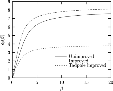
(b) SU(3)

(c) SU(4)

(d) SU(5)

Figure 1: Analytic calculation of the 2+1 dimensional unimproved, improved and tadpole improved vacuum energy density in units of $1/(aN_{p})$ for SU(2), SU(3), SU(4) and SU(5).

(a) SU(2)

(b) SU(3)

(c) SU(4)

(d) SU(5)

Figure 2: Analytic calculation of the unimproved, improved and tadpole improved variational parameter in 2+1 dimensions for SU(2), SU(3), SU(4) and SU(5).

IV.3 Dependence on truncation

In practice the $k$-sum appearing in the SU(3) generating function is truncated at a maximum value $k_{max}$. The dependence of the variational parameter on various truncations of the $k$-sum is shown in Fig. 3. We see that convergence is achieved up to $\beta\approx 13$ when keeping 20 terms. Further calculations show that when keeping 50 terms convergence up to $\beta\approx 30$ is achieved.

The $l$-sum appearing in the general SU($N$) generating function of Eq. (31) is also truncated in practice. We replace the infinite sum over $l$ by a sum from $-l_{\rm max}$ to $l_{\rm max}$. The dependence of the SU(3) and SU(4) variational parameters on $l_{\rm max}$ is shown in Fig. 4. From the graphs we see that convergence is achieved quickly as $l_{\rm max}$ increases for both SU(3) and SU(4). The results for $l_{\rm max}\geq 8$ are barely distinguishable up to $\beta=80$ with the scale used in the plots.

Figure 3: Analytic calculation of the unimproved SU(3) variational parameter in 2+1 dimensions, truncating the $k$-sum of ${\cal Y}(c,d)$ at $k=k_{max}$.

(a) SU(3)

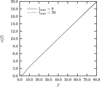
(b) SU(4)

Figure 4: Analytic calculation of the unimproved SU(3) and SU(4) variational parameters in 2+1 dimensions, truncating the $l$-sum of Eq. (31) at $l=\pm l_{max}$.

V Lattice Specific Heat

In addition to the vacuum energy density we can also calculate the lattice specific heat

$$C_{V}=-\frac{\partial^{2}\epsilon_{0}}{\partial\beta^{2}}.$$ (80)

The results for SU(2), SU(3), SU(4) and SU(5) are shown in Fig. 5. The SU(2) and SU(3) results are calculated with the aid of Eqs. (7) and (11) with the $k$-sum of Eq. (11) truncated at $k_{max}=50$. The SU(4) and SU(5) results are obtained using Eq. (31) to calculate the required matrix elements. For these cases the infinite $l$-sum is truncated at $l_{\rm max}=4$, for which the generating function has converged on the range of couplings used. We recall that the location of the peak indicates the region of transition from strong to weak coupling Horn et al. (1985). For an improved calculation one would expect the peak to be located at a smaller $\beta$ (corresponding to a larger coupling) than for the equivalent unimproved calculation. We see that this is indeed the case for each example, with the tadpole improved Hamiltonian demonstrating the largest degree of improvement.

(a) SU(2)

(b) SU(3)

(c) SU(4)

(d) SU(5)

Figure 5: The unimproved, improved and tadpole improved specific heat in 2+1 dimensions for SU(2), SU(3), SU(4) and SU(5).

VI Mass Gaps

VI.1 Introduction

Having fixed the one-plaquette vacuum wave function, in this section we turn to investigating excited states. Our aim is to calculate the lowest lying energy eigenstates of the Hamiltonians described by Eq. (76) for SU($N$) with $2\leq N\leq 5$.

We follow Arisue Arisue (1990) and expand the excited state $|\phi_{1}\rangle$ in the basis consisting of all rectangular Wilson loops $\{|n,m\rangle\}_{n,m=1}^{L_{max}}=\{|l\rangle\}_{l=1}^{L_{max}^{2}}$ that fit in a given square whose side length $L_{max}$ defines the order of the calculation. Enumerating the possible overlaps between rectangular loops is relatively simple and so a basis consisting of rectangular loops is an ideal starting point. However, for an accurate picture of the glueball spectrum we will need to extend the rectangular basis to include additional smaller area loops. Without such small area nonrectangular loops, it is possible that some of the lowest mass states will not appear in the variational calculation described here. In order to ensure the orthogonality of $|\phi_{0}\rangle$ and $|\phi_{1}\rangle$ we parameterise the excited state as follows

$$|\phi_{1}\rangle = \sum_{n,m=1}^{L_{max}}s_{l}|n,m\rangle=\sum_{l=1}^{L_{max}^{2}}s_{l}|l\rangle,$$ (81)

with,

$$|l\rangle = \sum_{\boldsymbol{x}}\left[W_{l}(\boldsymbol{x})-\langle W_{l}(\boldsymbol{x})\rangle\right]|\phi_{0}\rangle.$$ (82)

Here $\langle W_{l}(\boldsymbol{x})\rangle$ is the expectation value of $W_{l}(\boldsymbol{x})$ with respect to the ground state $|\phi_{0}\rangle$ and the convenient label $l=(n-1)L_{max}+m$ has been defined to label the $n\times m$ rectangular state, $|n,m\rangle$. We define the particular form of $W_{l}(\boldsymbol{x})$ to reflect the symmetry of the sector we wish to consider. For SU($N$) we take $W_{l}(\boldsymbol{x})={\rm Tr}[w_{l}(\boldsymbol{x})\pm w^{\dagger}_{l}(\boldsymbol{x})]$ for the symmetric ($0^{++}$) and antisymmetric ($0^{--}$) sectors. To avoid over-decorated equations, the particular $W_{l}(\boldsymbol{x})$ in use is to be deduced from the context. Here $w_{l}(\boldsymbol{x})$ is the rectangular Wilson loop joining the lattice sites $\boldsymbol{x}$, $\boldsymbol{x}+na\boldsymbol{i}$, $\boldsymbol{x}+na\boldsymbol{i}+ma\boldsymbol{j}$ and $\boldsymbol{x}+na\boldsymbol{j}$, with

$$n=\left[\frac{l-1}{L_{max}}\right]+1\quad{\rm and}\quad m=l-L_{max}\left[\frac{l-1}{L_{max}}\right].$$ (83)

Here $[k]$ denotes the integer part of $k$. In order to calculate excited state energies we minimise the mass gap (the difference between the excited state and ground state energies) over the basis defined by a particular order $L_{max}$. To do this we again follow Arisue Arisue (1990) and define the matrices

$$N_{ll^{\prime}} = \frac{1}{N_{p}}\langle l|\tilde{H}-E_{0}|l^{\prime}\rangle,$$ (84)

where $E_{0}$ is the ground state energy, and

$$D_{ll^{\prime}} = \frac{1}{N_{p}}\langle l|l^{\prime}\rangle=\sum_{\boldsymbol{x}}\left[\langle W^{\dagger}_{l}(\boldsymbol{x})W_{l^{\prime}}(\boldsymbol{0})\rangle-\langle W_{l}(\boldsymbol{x})\rangle^{\ast}\langle W_{l^{\prime}}(\boldsymbol{0})\rangle\right].$$ (85)

Extending the calculation to the general improved Hamiltonian $\tilde{H}(\kappa,u_{0})$ following Ref. Carlsson et al., 2002 gives

$$N_{ll^{\prime}} = -\frac{g^{2}}{2a}\sum_{i,\boldsymbol{x}}\sum_{\boldsymbol{x}^{\prime}}\Bigg{\{}(1-\kappa)\left\langle\left[E^{\alpha}_{i}(\boldsymbol{x}),W^{\dagger}_{l}(\boldsymbol{x}^{\prime})\right]\left[E^{\alpha}_{i}(\boldsymbol{x}),W_{l^{\prime}}(\boldsymbol{0})\right]\right\rangle$$ (86)

$$\hskip 56.9055pt+\frac{\kappa}{u_{0}^{2}}\left\langle\left[E^{\alpha}_{i}(\boldsymbol{x}),W^{\dagger}_{l}(\boldsymbol{x}^{\prime})\right]\left[\tilde{E}^{\alpha}_{i}(\boldsymbol{x}+a\boldsymbol{i}),W_{l^{\prime}}(\boldsymbol{0})\right]\right\rangle\Bigg{\}}.$$

To minimise the mass gap over a basis of a given order we make use of following diagonalisation technique Tonkin (1987). We first diagonalise $D$, with

$$S^{\dagger}DS=V^{2},$$ (87)

where $V$ is diagonal. The $n$-th lowest eigenvalue of the modified Hamiltonian

$$H^{\prime}=VS^{\dagger}NSV,$$ (88)

then gives an estimate for the mass gap corresponding to the $n$-th lowest eigenvalue of the Hamiltonian, $\Delta m_{n}$.

VI.2 Classification of states

States constructed from only gluon degrees of freedom can be classified in the continuum by their $J^{PC}$ quantum numbers. The assignment of $P$ and $C$ quantum numbers is straight forward Teper (1999). Care must be taken, however, when building states with particular continuum spins on the lattice. Difficulties arise when the continuous rotation group of the continuum is broken down to the group of lattice rotations. The most serious difficulty to arise is an ambiguity in the assignment of continuum spins to states built from lattice operators Teper (1999). To give a specific example, suppose we construct a wave function, $|\phi\rangle$, on the lattice with lattice spin $J=0$; a state built from Wilson loops which are unchanged by rotations of $n\pi/2$ for all integers $n$. As explained in Ref. Teper, 1999, this state is not a pure $J=0$ state; it also contains $J=4,8,\ldots$ states. Using a variational approach we can obtain estimates of the lowest energy eigenvalues of states with lattice spin $J=0$. When the continuum limit is taken we obtain estimates of the lowest continuum energy eigenvalues for the states with spin $0,4,8,\ldots$.

In the Lagrangian approach it is possible to suppress the unwanted spin $J\pm 4,J\pm 8,\ldots$ states in a given spin $J$ calculation. By “smearing” links, one can confidently construct lattice states which do not couple with the unwanted higher spin continuum states, at least for the lowest energy eigenvalues Teper (1999). The technique of “smearing” links has not to our knowledge been applied in the Hamiltonian approach.

Another way to clarify ambiguities in spin assignment is to attempt to construct a $J=4$ state on the lattice, devoid of $J=0$ contributions, and similarly a $J=0$ state devoid of unwanted $J=4$ contributions. The construction of an exact $J=4$ state is impossible on a square lattice due to the unavailability of $\pi/4$ rotations. One can however attempt to construct states that are approximately symmetric under rotations by $\pi/4$. In the Lagrangian approach in 2+1 dimensions, it has been demonstrated, for the simple case of SU(2), that such states can be chosen on a square lattice and that the approximate $\pi/4$ symmetry becomes exact in the continuum limit Johnson and Teper (1999). This technique is readily applicable in the Hamiltonian approach but has not yet been attempted.

Thus in our Hamiltonian calculation, which incorporates only rectangular states, a lattice spin $J$ state will correspond to a continuum state with spin $J,J\pm 4,J\pm 8,\ldots$. Using a variational approach we can obtain estimates of the lowest mass states in the continuum with these spin values. To improve the spin identification in the continuum beyond modulo $4$ requires more work. It will prove interesting to compare the masses calculated here to that of Teper Teper (1999) who has been careful to identify continuum spins correctly, at least for the lowest mass excitations.

VI.3 Calculating matrix elements

Having described the minimisation process we now detail the calculation of the matrix elements $N_{ll^{\prime}}$ and $D_{ll^{\prime}}$. Our aim is to reduce $N_{ll^{\prime}}$ and $D_{ll^{\prime}}$ to polynomials of one plaquette matrix elements. This, again has been done for the case of SU(2) by Arisue Arisue (1990). Here we retrace his calculations for the general case of SU($N$) and extend them to incorporate improved Hamiltonians. We start with $D_{ll^{\prime}}$.

Taking elementary plaquettes as our independent variables, it is easy to show that the only non-zero contributions to $D_{ll^{\prime}}$ occur when the rectangles $l$ and $l^{\prime}$ overlap. As an example of a contribution to $D_{ll^{\prime}}$, consider $\Delta D_{ll^{\prime}}$; the case where $N_{l\cap l^{\prime}}$ plaquettes are contained by both rectangles (these are the overlap plaquettes) and $N_{l}$ plaquettes are contained by the rectangle $l$. In order to calculate such matrix elements we rely heavily on the orthogonality properties of SU$(N)$ characters. We are interested in calculating SU$(N)$ integrals of the form

$$\int dU_{p}e^{S(U_{p})}\chi_{r}(U_{p}V),$$ (89)

where $U_{p}$ is a SU$(N)$ plaquette variable and $V$ is a product of any number of plaquettes not including $U_{p}$. Here $\chi_{r}(U)$ denotes the character corresponding to the representation $r$. For SU(2), $r=0,1/2,3/2,\ldots$ and for SU(3), $r=(\lambda,\mu)$ where $\lambda$ denotes the number of boxes in the first row of the Young tableau describing the representation and $\mu$ is the number of boxes in the second row. Similarly, for SU$(N)$, $r=(r_{1},r_{2},\ldots,r_{N-1})$.

Performing a character expansion of the exponential in Eq. (89) gives:

$$\int dU_{p}e^{S(U_{p})}\chi_{r}(U_{p}V) = \sum_{r^{\prime}}\int dU_{p}c_{r^{\prime}}\chi_{r^{\prime}}(U_{p})\chi_{r}(U_{p}V).$$ (90)

This is simply a generalisation of a Fourier expansion. Here, the coefficient $c_{r^{\prime}}$ is given by:

$$c_{r^{\prime}}=\int dU_{p}\chi_{r^{\prime}}(U_{p})e^{S(U_{p})}.$$ (91)

Now, using the orthogonality relation,

$$\int dU_{p}\chi_{r^{\prime}}(U_{p}V)\chi_{r}(U_{p})=\frac{1}{d_{r}}\delta_{r^{\prime}r}\chi_{r}(V),$$ (92)

where $d_{r}$ is the dimension of the representation $r$, we obtain:

$$\int dU_{p}e^{S(U_{p})}\chi_{r}(U_{p}V) = \frac{1}{d_{r}}\chi_{r}(V)\int dU_{p}\chi_{r}(U_{p})e^{S(U_{p})}.$$ (93)

This result allows us to integrate out a single plaquette from an extended Wilson loop in a given representation $r$. To complete the calculation we need to relate SU($N$) characters to the traces of group elements. This can be done using Weyl’s character formula Bars (1980). For SU($N$), according to Bars Bars (1980), the dimensions and characters corresponding to the first few representations are given by:

$$\begin{array}[]{rclrcl}\displaystyle\chi_{1}(U)&=&{\rm Tr}U&\displaystyle d_{1}(U)&=&N\vspace{0.1cm}\\ \chi_{2}(U)&=&\displaystyle\frac{1}{2}\left[({\rm Tr}U)^{2}+{\rm Tr}U^{2}\right]&d_{2}(U)&=&\displaystyle\frac{1}{2}N(N+1)\vspace{0.1cm}\\ \displaystyle\chi_{11}(U)&=&\displaystyle\frac{1}{2}\left[({\rm Tr}U)^{2}-{\rm Tr}U^{2}\right]&d_{11}(U)&=&\displaystyle\frac{1}{2}N(N-1)\vspace{0.1cm}\\ \chi_{21}(U)&=&\displaystyle\frac{1}{3}\left[({\rm Tr}U)^{3}-{\rm Tr}U^{3}\right]&d_{21}(U)&=&\displaystyle\frac{1}{3}(N-1)N(N+1)\vspace{0.1cm}\\ \displaystyle\chi_{1^{N-1}}(U)&=&\displaystyle{\rm Tr}U^{\dagger}&\displaystyle d_{1^{N-1}}(U)&=&N\end{array}$$ (99)

Here we have adopted the convention of dropping all zeros in the character labels. The Mandelstam constraints for the gauge group in question allows all characters to be expressed in terms of a minimal set of trace variables. For example, for SU(3) we make use of the Mandelstam constraint,

$${\rm Tr}(A^{2}B)={\rm Tr}A{\rm Tr}(AB)-{\rm Tr}A^{\dagger}{\rm Tr}B+{\rm Tr}(A^{\dagger}B),$$ (100)

where $A\in{\rm SU}(3)$ and $B$ is any $3\times 3$ matrix, to express all characters in terms of ${\rm Tr}U$ and ${\rm Tr}U^{\dagger}$. For example, for the case of SU(3), Eq. (99) simplifies to

$$\begin{array}[]{rclcrcl}\displaystyle\chi_{1}(U)&=&{\rm Tr}U&&d_{1}&=&3\\ \vspace{0.1cm}\displaystyle\chi_{11}(U)&=&\displaystyle\displaystyle\frac{1}{2}\left[({\rm Tr}U)^{2}-{\rm Tr}(U^{2})\right]={\rm Tr}U^{\dagger}&&d_{11}&=&3\\ \displaystyle\vspace{0.1cm}\chi_{2}(U)&=&\displaystyle\displaystyle\frac{1}{2}\left[({\rm Tr}U)^{2}+{\rm Tr}(U^{2})\right]=({\rm Tr}U)^{2}-{\rm Tr}U^{\dagger}&&d_{2}&=&6\\ \displaystyle\chi_{21}(U)&=&\displaystyle\displaystyle\frac{1}{3}\left[({\rm Tr}U)^{3}-{\rm Tr}(U^{3})\right]={\rm Tr}U{\rm Tr}U^{\dagger}-1&&d_{21}&=&8\end{array}$$ (105)

However, for general SU($N$) the Mandelstam constraints are difficult to calculate. In what follows we will need expressions for ${\rm Tr}U$, ${\rm Tr}U^{\dagger}$, ${\rm Tr}(U^{2})$, $({\rm Tr}U)^{2}$, and ${\rm Tr}U{\rm Tr}U^{\dagger}$ as linear combinations of characters for SU($N$). It is possible to do this without the use of the Mandelstam constraint. Such expressions are necessary in order to make use of Eq. (93) in the calculation of expectation values of trace variables. For ${\rm Tr}U$, ${\rm Tr}U^{\dagger}$, ${\rm Tr}(U^{2})$ and $({\rm Tr}U)^{2}$ the necessary expressions are easily obtained by rearranging Eq. (99),

$${\rm Tr}U = \chi_{1}(U)$$

$$({\rm Tr}U)^{2} = \chi_{2}(U)+\chi_{11}(U)$$

$${\rm Tr}U^{2} = \chi_{2}(U)-\chi_{11}(U)$$

$${\rm Tr}U^{\dagger} = \chi_{1^{N-1}}(U).$$ (106)

To express the remaining expression, ${\rm Tr}U{\rm Tr}U^{\dagger}$, as a linear combination of characters is not as easily done. For SU(3) one can simply rearrange the expression for $\chi_{21}(U)$ in Eq. (105). For the general $N$ case it is simplest to consider Young tableaux. In terms of Young tableaux we have

$${\rm Tr}U{\rm Tr}U^{\dagger}\equiv\square\,\otimes\left.\begin{array}[]{c}\square\vspace{-0.18cm}\\ \square\vspace{-0.18cm}\\ \vdots\\ \square\end{array}\right\}N-1.$$ (111)

Performing the product representation decomposition gives

$$\square\,\otimes\left.\begin{array}[]{c}\square\vspace{-0.18cm}\\ \square\vspace{-0.18cm}\\ \vdots\\ \square\end{array}\right\}N-1 = \left.\begin{array}[]{c}\square\vspace{-0.18cm}\\ \square\vspace{-0.18cm}\\ \vdots\\ \square\end{array}\right\}N+\left.\begin{array}[]{c c}\square\vspace{-0.18cm}&\square\\ \square\vspace{-0.18cm}\\ \vdots\\ \square\end{array}\right\}N-1$$ (124)

Converting back into the notation of characters and traces gives

$${\rm Tr}U{\rm Tr}U^{\dagger} = 1+\chi_{21^{N-2}}(U).$$ (125)

Eqn(125) together with Eqs. (106) and (93) allow the analytic calculation of each contribution to $D_{ll^{\prime}}$ for all $N$. For the case of $\Delta D_{ll^{\prime}}$ described earlier, we have

$$\Delta D_{ll^{\prime}}=\frac{2}{N}F_{Z_{1}}(N_{l}+N_{l^{\prime}}-2N_{l\cap l^{\prime}})\left[F_{Z_{1}^{2}}(N_{l\cap l^{\prime}})+F_{Z_{1}\!\bar{Z}_{1}}(N_{l\cap l^{\prime}})\right]-4F_{Z_{1}}(N_{l})F_{Z_{1}}(N_{l^{\prime}}),$$ (126)

where the character integrals are defined by:

$$F_{Z_{1}}(n) \!\!\!=\!\!\! \left(\frac{1}{N}\right)^{n-1}\langle Z_{1}\rangle^{n},$$ (127)

$$F_{Z_{1}^{2}}(n) \!\!\!=\!\!\! \frac{1}{2}\left[\frac{1}{N(N+1)}\right]^{n-1}\langle Z_{1}^{2}+Z_{2}\rangle^{n}+\frac{1}{2}\left[\frac{1}{N(N-1)}\right]^{n-1}\langle Z_{1}^{2}-Z_{2}\rangle^{n},$$ (128)

$$F_{Z_{2}}(n) \!\!\!=\!\!\! \frac{1}{2}\left[\frac{1}{N(N+1)}\right]^{n-1}\langle Z_{1}^{2}+Z_{2}\rangle^{n}-\frac{1}{2}\left[\frac{1}{N(N-1)}\right]^{n-1}\langle Z_{1}^{2}-Z_{2}\rangle^{n},$$ (129)

$$F_{Z_{1}\bar{Z}_{1}}(n) \!\!\!=\!\!\! 1+\left[\frac{1}{(N-1)(N+1)}\right]^{n-1}\left(\langle Z_{1}\bar{Z}_{1}\rangle-1\right)^{n}.$$ (130)

Here we have made use of the notation, $Z_{n}:={\rm Tr}\left(U^{n}\right)$, to denote the trace variables occupying a single plaquette, $U$. The expectation values appearing in Eq. (130) are easily expressed in terms of the generating functions of Eqs. (31) and (74). Differentiating the generating functions appropriately gives

$$\langle Z_{1}\rangle = \frac{1}{G_{{\rm SU}(N)}}\frac{\partial G_{{\rm SU}(N)}}{\partial c}\Bigg{|}_{d=c}$$

$$\langle Z_{1}\bar{Z}_{1}\rangle = \frac{1}{G_{{\rm SU}(N)}}\frac{\partial^{2}G_{{\rm SU}(N)}}{\partial c\partial d}\Bigg{|}_{d=c}$$

$$\langle Z_{1}^{2}\pm Z_{2}\rangle = \frac{1}{G_{{\rm SU}(N)}}\frac{\partial^{2}G_{{\rm SU}(N)}}{\partial c^{2}}\Bigg{|}_{d=c}\pm\frac{1}{H_{2}}\frac{\partial H_{2}}{\partial d}\Bigg{|}_{d=0}.$$ (131)

In practice, we do not need to calculate all of these matrix elements. We see from Eq. (31) that $\langle Z_{1}^{2}\rangle$ and $\langle Z_{1}\bar{Z}_{1}\rangle$ are related by

$$\langle Z_{1}^{2}\rangle = \frac{1}{2}\frac{d^{2}\langle Z_{1}\rangle}{dc^{2}}-\langle Z_{1}\bar{Z}_{1}\rangle.$$ (132)

This follows from the fact that a group integral does not depend on the choice of direction for the links. To be more precise, the result,

$$\int_{{\rm SU}(N)}dUf(U)=\int_{{\rm SU}(N)}dU^{\dagger}f(U^{\dagger})=\int_{{\rm SU}(N)}dUf(U^{\dagger}),$$ (133)

follows from the fact that $dU^{\dagger}$ and $dU$ each define invariant Haar measures on SU($N$) which, by uniqueness, must be equal.

We now move on to the calculation of $N_{ll^{\prime}}$. It is easy to show that the only non-zero contributions occur when there is at least one common link and an overlap between the rectangles. The improvement term (the second term in Eq. (86)) only contributes when the two rectangles share at least two neighbouring links in a given direction. Consider the contribution $\Delta N_{ll^{\prime}}$ to $N_{ll^{\prime}}$ in which there are $L_{1}$ common links and $L_{2}$ common strings of two links in a given direction. Again we suppose $N_{l}$ plaquettes are enclosed by rectangle $l$ and that there are $N_{l\cap l^{\prime}}$ common plaquettes. Making use of Eq. (93) and following Ref. Carlsson et al., 2002 we obtain

$$\Delta N_{ll^{\prime}}=\frac{L}{N}F_{Z_{1}}(N_{l}\!+\!N_{l^{\prime}}\!-\!2N_{l\cap l^{\prime}})\left[F_{Z_{2}}(N_{l\cap l^{\prime}})\!-\!\frac{1}{N}F_{Z_{1}^{2}}(N_{l\cap l^{\prime}})\!-\!N\!+\!\frac{1}{N}F_{Z_{1}\!\bar{Z}_{1}}(N_{l\cap l^{\prime}})\right],$$ (134)

with

$$L=(1-\kappa)L_{1}+\frac{\kappa}{u_{0}^{2}}L_{2}.$$ (135)

For the case of SU(3) we can simplify this using Eq. (100) to

$$\Delta N_{ll^{\prime}}=\frac{L}{3}F_{Z_{1}}(N_{l}\!+\!N_{l^{\prime}}\!-\!2N_{l\cap l^{\prime}})\left[\frac{2}{3}F_{Z_{1}^{2}}(N_{l\cap l^{\prime}})\!-\!2F_{Z_{1}}(N_{l\cap l^{\prime}})\!-\!3\!+\!\frac{1}{3}F_{Z_{1}\!\bar{Z}_{1}}(N_{l\cap l^{\prime}})\right].$$ (136)

Having determined individual contributions to $D_{ll^{\prime}}$ and $N_{ll^{\prime}}$, to complete their calculation the possible overlaps between states $l$ and $l^{\prime}$ of a given type must be counted.

VI.4 Choosing an appropriate vacuum state

In Section IV we calculated variational vacuum wave functions for pure SU($N$) gauge theory for $N=2$, 3, 4 and 5. Our motivation was to use these wave functions as inputs to calculations of SU($N$) massgaps. We obtained wave functions with a variational parameter that was proportional to $\beta$ in the large $\beta$ limit and $\beta^{2}$ in the small $\beta$ limit. However, this behaviour is incompatible with the exact continuum vacuum wave function. For a one-plaquette trial state, given by Eq. (1), to be compatible with the exact continuum vacuum wave function in 2+1 dimensions, one must have $c\propto\beta^{2}$ in the large $\beta$ limit Greensite (1987). This result is independent of the dimension of the gauge group in question. For the case of SU(2) in 2+1 dimensions, in the scaling region it has been shown Greensite (1987) that for compatibility with the exact SU(2) continuum vacuum wave function, we must use the Greensite vacuum wave function

$$\begin{array}[]{c}\includegraphics{thesis-paper1-eqn92.eps}\end{array}$$ (137)

It is this vacuum wave function that was used by Arisue Arisue (1990) in the calculation that we generalise in this paper. It would thus seem that using a variational wave function is not appropriate in the calculation of massgaps. However, the scaling argument presented in Ref. Carlsson et al., 2002 demonstrates that in a glueball mass scaling region the precise form of $c(\beta)$ is not important. For this reason we expect that the results presented here will agree with a calculation using the Greensite wave function.

As it turns out, to calculate variational wave functions for large dimension gauge groups is cumbersome. Numerical precision becomes a factor in the minimisation of the energy density. This problem is magnified in the calculation of tadpole improved results. We thus abandon the use of variational wave functions in the calculation of massgaps beyond SU(5). Instead we make use of the one plaquette wave function of Eq. (1) and define a simple dependence, $c(\beta)$, which most often will be $c(\beta)=\beta$. Calculations for $N>5$ will be presented in a later publication.

VII SU(2), SU(3), SU(4) and SU(5) Massgap Results

In this section we present glueball mass results for SU($N$) pure gauge theory in 2+1 dimensions with $N=2$, 3, 4 and 5. For each SU(3) calculation we keep 80 terms in the $k$-sum of Eq. (11) giving convergence up to $\beta=50$. For $N>3$ the truncation $l_{{\rm max}}=20$ is used. The generation of $N_{ll^{\prime}}$ and $D_{ll^{\prime}}$ and implementation of the minimisation process is accomplished with a Mathematica code.

For the case of 2+1 dimensions we expect $a\Delta m/g^{2}$ to become constant in the scaling region. The convergence of the massgaps with $L_{max}$ is illustrated in Fig. 6. We notice that for $N>2$ only small improvements to the scaling behaviour are gained by extending the calculation beyond order 8 on the range of couplings shown. This suggests that a more complicated basis (including, for example, nonrectangular loops) is required to simulate SU($N$) excited states with $N>2$ than for the case of SU(2).

(a) SU(2)

(b) SU(3)

(c) SU(4)

(d) SU(5)

Figure 6: The unimproved 2+1 dimensional symmetric massgaps for SU(2), SU(3), SU(4) and SU(5).

In Fig. 7 results for the lowest lying glueball mass, calculated with Kogut-Susskind, improved and tadpole Hamiltonians, are shown. We see that $a\Delta m^{S}_{1}/g^{2}$ is approximated well by a constant, in very large scaling regions, for the lowest lying eigenstates for all $N$ considered. The scaling behavior becomes significantly worse for the antisymmetric sector which is shown in Fig. 8 and for higher energy eigenvalues. This is because the simplistic form of our excited state wave function is not sufficient to reproduce the plaquette correlations required to simulate these higher order states. One would expect the simulation of higher order eigenstates to improve by including more complicated loops in our expansion basis or by using a more complicated ground state. The continuum limit excited states results for SU($N$) are given in Tables 1—7.

For the unimproved SU(2) case, the masses of the lowest two eigenstates agree closely with the calculations of Arisue Arisue (1990) (respectively $2.056\pm 0.001$ and $3.64\pm 0.03$ in units of $e^{2}=g^{2}/a$) in which the Greensite vacuum wave function of Eq. (137) was used. This serves as a check on our counting in calculating the possible overlaps of excited states. Our calculation is in disagreement with that of Arisue at the third eigenstate, for which Arisue calculates a mass $(5.15\pm 0.1)e^{2}$. Our fourth eigenstate is close in mass to Arisue’s third and our third eigenstate does not appear in his results. The reasons for this are not clear.

The results for the SU(3) symmetric massgap (in units of $e^{2}$) are to be compared to calculations by Luo and Chen $2.15\pm 0.06$ Luo and Chen (1996), Samuel $1.84\pm 0.46$ Samuel (1997) and Teper $2.40\pm 0.02$ Teper (1999). Our result of $3.26520\pm 0.00009$ is considerably higher than all existing comparable results. By including more complicated loops in the expansion basis one would expect to reduce this estimate. This is emphasised by the fact that when using only square basis states our result is considerably higher. To explain the discrepancy between the our results and other’s it is important to note that since we use a basis of rectangles we exclude the contribution of many non-rectangular small area diagrams that are included in the calculations of Teper and that of Luo and Chen. For this reason it may be the case that what we have interpretted as the lowest glueball mass in this paper may, in fact, be a higher order excited state. Teper has calculated the masses of the three lowest mass glueballs for SU(3) in the $0^{++}$ sector Teper (1999): $0^{++}$, $0^{++*}$ and $0^{++**}$, with the respective results, in units of $e^{2}$: $2.40\pm 0.02$, $3.606\pm 0.063$ and $4.55\pm 0.11$. It is interesting to note that our result is closer to Teper’s first excited state. In the same study Teper also calculated glueball masses in the $0^{++}$ sector for $N=4$, 5 and 6. The mass, in units of $e^{2}$, of his $0^{++*}$ state for SU(4) is $4.84\pm 0.12$ and $5.99\pm 0.16$ for SU(5). We notice that as $N$ is increased the results presented here move closer to the mass of Teper’s $0^{++*}$ state, with the improved results being closer than the unimproved. In fact for SU(5), the results presented here, improved and unimproved, are consistent with Teper’s $0^{++*}$ mass. This forces us to question the interpretation of the large $\beta$ plateaux in Fig. 7 as scaling regions for the lowest mass glueballs. It is possible that the minima present in Fig. 7 in the small $\beta$ region are possible scaling regions. It is possible that our vacuum wave function and minimisation basis are insufficient to extend this scaling region over a wide range of couplings and that as our approximation breaks down we observe a level crossing effect. We will examine the possibility of the small $\beta$ minima being scaling regions in a later publication.

The antisymmetric results presented here can also be compared with those of Teper Teper (1999). While each of our results is considerably higher than the masses of Teper’s $0^{--}$ and $0^{--*}$ states, Teper’s $0^{--**}$ state has a mass which is close to the lowest mass state calculated here. Teper obtains the following masses, in units of $e^{2}$, for the $0^{--**}$ state: $5.42\pm 0.16$ for SU(3), $6.98\pm 0.26$ for SU(4) and $9.18\pm 0.45$ for SU(5). It is interesting to note that our corresponding lowest unimproved glueball masses are consistent with these results. Our improved results show better agreement with Teper’s $0^{--**}$ state for SU(3) and SU(5) than the corresponding unimproved results. The improved SU(4) results are also consistent with Teper’s SU(4) $0^{--**}$ mass although the agreement is closer for the unimproved result.

(a) Symmetric SU(2) massgap

(b) Symmetric SU(3) massgap

(c) Symmetric SU(4) massgap

(d) Symmetric SU(5) massgap

Figure 7: 2+1 dimensional symmetric massgaps for SU(2), SU(3) (both with $L_{max}=25$), SU(4) (with $L_{max}=16$) and SU(5) (with $L_{max}=12$).

(a) Antisymmetric SU(3) massgap

(b) Antisymmetric SU(4) massgap

(c) Antisymmetric SU(5) massgap

Figure 8: 2+1 dimensional antisymmetric massgaps for SU(3) (with $L_{max}=25$), SU(4) and SU(5) (both with $L_{max}=12$).

Table 1: Estimates of the lowest lying SU(2) glueball masses (in units of $e^{2}$) computed with various Hamiltonians in 2+1 dimensions. The unimproved, improved and tadpole results are calculated in the respective scaling regions $13.5\leq\beta\leq 30.0$, $9.9\leq\beta\leq 30.0$ and $9.25\leq\beta\leq 30.0$.

	Unimproved	Improved	Tadpole Improved
$\Delta m^{S}_{1}$	$2.05691\mbox{$\pm$}0.00002$	$2.0897\mbox{$\pm$}0.0003$	$2.0965\mbox{$\pm$}0.0006$
$\Delta m^{S}_{2}$	$3.645\mbox{$\pm$}0.001$	$3.685\mbox{$\pm$}0.001$	$3.6953\mbox{$\pm$}0.0009$
$\Delta m^{S}_{3}$	$4.5202\mbox{$\pm$}0.0004$	$4.574\mbox{$\pm$}0.004$	$4.583\mbox{$\pm$}0.004$
$\Delta m^{S}_{4}$	$5.133\mbox{$\pm$}0.003$	$5.177\mbox{$\pm$}0.004$	$5.189\mbox{$\pm$}0.004$
$\Delta m^{S}_{5}$	$5.867\mbox{$\pm$}0.006$	$5.932\mbox{$\pm$}0.008$	$5.943\mbox{$\pm$}0.008$

Table 2: Estimates of the lowest lying symmetric SU(3) glueball masses (in units of $e^{2}$) computed with various Hamiltonians in 2+1 dimensions. The results are calculated in the scaling region which minimises the standard error in each case.

	Unimproved	Improved	Tadpole Improved
$\Delta m^{S}_{1}$	$3.265868\mbox{$\pm$}0.000042$	$3.32365\mbox{$\pm$}0.00012$	$3.32580\mbox{$\pm$}0.00015$
$\Delta m^{S}_{2}$	$6.23903\mbox{$\pm$}0.00065$	$6.30391\mbox{$\pm$}0.00083$	$6.31192\mbox{$\pm$}0.00084$
$\Delta m^{S}_{3}$	$7.5767\mbox{$\pm$}0.0025$	$7.6466\mbox{$\pm$}0.0030$	$7.6498\mbox{$\pm$}0.0030$
$\Delta m^{S}_{4}$	$8.9462\mbox{$\pm$}0.0029$	$9.0118\mbox{$\pm$}0.0044$	$9.0206\mbox{$\pm$}0.0045$
$\Delta m^{S}_{5}$	$10.0778\mbox{$\pm$}0.0071$	$10.1546\mbox{$\pm$}0.0094$	$10.1628\mbox{$\pm$}0.0094$

Table 3: Estimates of the lowest lying symmetric SU(4) massgaps (in units of $e^{2}$) computed with various Hamiltonians in 2+1 dimensions. The results are calculated in the scaling region which minimises the standard error in each case.

	Unimproved	Improved	Tadpole Improved
$\Delta m^{S}_{1}$	$4.59121\mbox{$\pm$}0.00007$	$4.6720\mbox{$\pm$}0.0001$	$4.6754\mbox{$\pm$}0.0001$
$\Delta m^{S}_{2}$	$8.8122\mbox{$\pm$}0.0012$	$8.9276\mbox{$\pm$}0.0016$	$8.9284\mbox{$\pm$}0.0017$
$\Delta m^{S}_{3}$	$10.5889\mbox{$\pm$}0.0051$	$10.7807\mbox{$\pm$}0.0051$	$10.7794\mbox{$\pm$}0.0051$
$\Delta m^{S}_{4}$	$12.5527\mbox{$\pm$}0.0048$	$12.6266\mbox{$\pm$}0.0081$	$12.6138\mbox{$\pm$}0.0080$
$\Delta m^{S}_{5}$	$14.052\mbox{$\pm$}0.012$	$14.165\mbox{$\pm$}0.016$	$14.157\mbox{$\pm$}0.016$

Table 4: Estimates of the lowest lying symmetric SU(5) massgaps (in units of $e^{2}$) computed with various Hamiltonians in 2+1 dimensions. The results are calculated in the scaling region which minimises the standard error in each case.

	Unimproved	Improved	Tadpole Improved
$\Delta m^{S}_{1}$	$5.8903\mbox{$\pm$}0.0001$	$5.99434\mbox{$\pm$}0.00009$	$5.9983\mbox{$\pm$}0.0002$
$\Delta m^{S}_{2}$	$11.2335\mbox{$\pm$}0.0036$	$11.3696\mbox{$\pm$}0.0050$	$11.3731\mbox{$\pm$}0.0049$
$\Delta m^{S}_{3}$	$13.340\mbox{$\pm$}0.011$	$13.658\mbox{$\pm$}0.012$	$13.663\mbox{$\pm$}0.011$
$\Delta m^{S}_{4}$	$15.881\mbox{$\pm$}0.012$	$15.890\mbox{$\pm$}0.019$	$15.890\mbox{$\pm$}0.019$
$\Delta m^{S}_{5}$	$17.564\mbox{$\pm$}0.025$	$17.676\mbox{$\pm$}0.035$	$17.682\mbox{$\pm$}0.035$

Table 5: Estimates of the lowest lying antisymmetric SU(3) massgaps (in units of $e^{2}$) computed with various Hamiltonians in 2+1 dimensions. The results are calculated in the scaling region which minimises the standard error in each case.

	Unimproved	Improved	Tadpole Improved
$\Delta m^{A}_{1}$	$5.32750\mbox{$\pm$}0.00047$	$5.39661\mbox{$\pm$}0.00034$	$5.39864\mbox{$\pm$}0.00032$
$\Delta m^{A}_{2}$	$7.9389\mbox{$\pm$}0.0021$	$8.0142\mbox{$\pm$}0.0028$	$8.0145\mbox{$\pm$}0.0028$
$\Delta m^{A}_{3}$	$8.9319\mbox{$\pm$}0.0045$	$9.0092\mbox{$\pm$}0.0056$	$9.0087\mbox{$\pm$}0.0055$
$\Delta m^{A}_{4}$	$10.4711\mbox{$\pm$}0.0058$	$10.5514\mbox{$\pm$}0.0085$	$10.5502\mbox{$\pm$}0.0085$
$\Delta m^{A}_{5}$	$11.304\mbox{$\pm$}0.011$	$11.384\mbox{$\pm$}0.015$	$11.381\mbox{$\pm$}0.015$

Table 6: Estimates of the lowest lying antisymmetric SU(4) massgaps (in units of $e^{2}$) computed with various Hamiltonians in 2+1 dimensions. The results are calculated in the scaling regions which minimise the standard error in each case.

	Unimproved	Improved	Tadpole Improved
$\Delta m^{A}_{1}$	$7.21479\mbox{$\pm$}0.0012$	$7.3310\mbox{$\pm$}0.0011$	$7.33586\mbox{$\pm$}0.00077$
$\Delta m^{A}_{2}$	$10.9117\mbox{$\pm$}0.0033$	$11.0099\mbox{$\pm$}0.004909$	$11.0617\mbox{$\pm$}0.0046$
$\Delta m^{A}_{3}$	$12.121\mbox{$\pm$}0.007$	$12.2779\mbox{$\pm$}0.0088$	$12.292\mbox{$\pm$}0.009$
$\Delta m^{A}_{4}$	$14.5012\mbox{$\pm$}0.0089$	$14.592\mbox{$\pm$}0.014$	$14.574\mbox{$\pm$}0.015$
$\Delta m^{A}_{5}$	$15.4521\mbox{$\pm$}0.0173$	$15.545\mbox{$\pm$}0.023$	$15.555\mbox{$\pm$}0.023$

Table 7: Estimates of the lowest lying antisymmetric SU(5) massgaps (in units of $e^{2}$) computed with various Hamiltonians in 2+1 dimensions. The results are calculated in the scaling regions which minimise the standard error in each case.

	Unimproved	Improved	Tadpole Improved
$\Delta m^{A}_{1}$	$9.067\mbox{$\pm$}0.003$	$9.239\mbox{$\pm$}0.002$	$9.248\mbox{$\pm$}0.002$
$\Delta m^{A}_{2}$	$13.717\mbox{$\pm$}0.008$	$13.89\mbox{$\pm$}0.01$	$13.89\mbox{$\pm$}0.01$
$\Delta m^{A}_{3}$	$15.054\mbox{$\pm$}0.015$	$15.32\mbox{$\pm$}0.02$	$15.327\mbox{$\pm$}0.019$
$\Delta m^{A}_{4}$	$18.08\mbox{$\pm$}0.02$	$18.12\mbox{$\pm$}0.03$	$18.12\mbox{$\pm$}0.03$
$\Delta m^{A}_{5}$	$19.084\mbox{$\pm$}0.036$	$19.19\mbox{$\pm$}0.05$	$19.20\mbox{$\pm$}0.05$

When compared to equivalent unimproved calculations, the improved and tadpole improved massgaps approach scaling faster as $\beta$ is increased. This is evident in Figs. 6 and 7 and is expected since, for an improved calculation one is closer to the continuum limit when working at a given coupling. However, for most improved calculations the scaling behaviour is marginally less precise than the equivalent unimproved calculation. A possible reason for this is that the one plaquette trial state used here does not allow for direct contributions from the improvement term in the kinetic Hamiltonian. For this term to contribute directly one would need a trial state which includes Wilson loops extending at least two links in at least one direction.

The improved SU(2) massgap can be compared to the coupled cluster calculation of Li et al Li et al. (2000). Their result (in units of $e^{2}$), $\Delta m^{S}_{1}=1.59$, is again significantly lower than our result $2.0897\pm 0.0003$. The difference is again attributable to the different choices of Wilson loops used in the simulation of states. While our calculation makes use of the simple one plaquette ground state and a minimisation basis with only rectangular loops, the coupled cluster calculation of Li et al uses a more accurate ground state wave function consisting of an exponential of a sum of extended loops which are not necessarily rectangular. Without including additional small area Wilson loops we cannot be confident that the lowest mass state accessible with our minimisation basis is in fact the lowest mass state of the theory. Clearly there is scope for more work here.

VIII Conclusion

In this paper we have extended the analytic techniques of 2+1 dimensional Hamiltonian LGT, traditionally used for SU(2), to general SU($N$). Impressive scaling is achieved over an extremely wide range of couplings for the lowest energy eigenstates in the symmetric and antisymmetric sectors. Our calculations use a one plaquette trial state and a basis of rectangular states over which excited state energies are minimised. Such choices allow the use of analytic techniques in SU($N$) calculations.

The results of this paper give estimates of the lowest unimproved, improved and tadpole improved SU($N$) glueball masses, all of which are above current estimates. We suspect that the reason for the discrepancy is a lack of small area non-rectangular states in our minimisation basis. A basis of rectangular states was used for simplicity. The inclusion of non-rectangular states is straightforward and only complicates the counting of overlaps between diagrams of a particular type. When not including sufficient small area diagrams it is possibly that the lowest mass states of the theory are not accessible over a large range of couplings. A further improvement to our calculation would involve the use of an improved trial vacuum state. Such a state would possibly include several extended Wilson loops in its exponent. Without the development of new techniques for performing the required integrals the use of such a vacuum wave function would require the use of Monte Carlo techniques for the calculation of expectation values. In this scenario many advantages of the Hamiltonian approach would be lost.

In a later publication we extend the calculations presented here to SU(25) in an attempt to explore the mass spectrum in the large $N$ limit of pure SU($N$) gauge theory.

References

• Carlsson et al. (2002) J. Carlsson, J. A. L. McIntosh, B. H. J. McKellar, and L. C. L. Hollenberg (2002), eprint hep-lat/0207019.
• Kogut and Susskind (1975) J. B. Kogut and L. Susskind, Phys. Rev. D11, 395 (1975).
• Carlsson and McKellar (2001) J. Carlsson and B. H. J. McKellar, Phys. Rev. D64, 094503 (2001), eprint hep-lat/0105018.
• Montvay and Münster (1994) I. Montvay and G. Münster, Quantum Fields on a Lattice (Cambridge University Press, 1994), chap. 3.2.3, (Cambridge Monographs On Mathematical Physics).
• Creutz (1983) M. Creutz, Quarks, Gluons and Lattices (Cambridge University Press, 1983), (Cambridge Monographs On Mathematical Physics).
• Batrouni and Halpern (1984) G. G. Batrouni and M. B. Halpern, Phys. Rev. D30, 1782 (1984).
• Arisue et al. (1983) H. Arisue, M. Kato, and T. Fujiwara, Prog. Theor. Phys. 70, 229 (1983).
• Eriksson et al. (1981) K. E. Eriksson, N. Svartholm, and B. S. Skagerstam, J. Math. Phys. 22, 2276 (1981).
• Baik and Rains (2001) J. Baik and E. M. Rains, Duke Math. J. 2, issue 1:1 (2001), eprint [http://arXiv.org/abs]math.CO/9905083.
• Rains (1998) E. M. Rains, Electron. J. Combin. 5(1), R12 (1998).
• Widom et al. (2001) H. Widom, A. R. Its, and C. A. Tracy, Physica D152-153, 199 (2001).
• Regev (1981) A. Regev, Adv. in Math. 41, 115 (1981).
• Gessel (1990) I. M. Gessel, J. Combin. Theory Ser. A 53, 257 (1990).
• Diaconis and Shahshahani (1994) P. Diaconis and M. Shahshahani, J. Appl. Probab. 31A, 49 (1994).
• Widom and Tracy (1999) H. Widom and C. A. Tracy, Comm. Math. Phys. 207, 665 (1999).
• Creutz (1978) M. Creutz, J. Math. Phys. 19, 2043 (1978).
• Leonard (2001) C. R. Leonard, Ph.D. thesis, The University of Melbourne (2001).
• De Pietri (1997) R. De Pietri, Class. Quant. Grav. 14, 53 (1997), eprint [http://arXiv.org/abs]gr-qc/9605064.
• Rovelli and Smolin (1995) C. Rovelli and L. Smolin, Phys. Rev. D52, 5743 (1995), eprint [http://arXiv.org/abs]gr-qc/9505006.
• Ezawa (1997) K. Ezawa, Phys. Rept. 286, 271 (1997), eprint [http://arXiv.org/abs]gr-qc/9601050.
• Kogut et al. (1982) J. B. Kogut, M. Snow, and M. Stone, Nucl. Phys. B200, 211 (1982).
• Brower et al. (1981) R. Brower, P. Rossi, and C.-I. Tan, Nucl. Phys. B190, 699 (1981).
• Weyl (1946) H. Weyl, The Classical Groups, Their Invariants and Representations (Princeton University Press, 1946).
• Gradshteyn and Ryzhik (1994) I. S. Gradshteyn and I. M. Ryzhik, Table of Integrals, Series, and Products (Academic Press, 1994).
• van Moerbeke (2001) P. van Moerbeke, in Random Matrices and Their Applications (Cambridge University Press, 2001), MSRI-publication #40, eprint [http://arXiv.org/abs]math.CO/0010135.
• (26) N. J. A. Sloane, The On-line Encyclopedia of Integer Sequences, eprint http://www.research.att.com/~njas/sequences/.
• Horn et al. (1985) D. Horn, M. Karliner, and M. Weinstein, Phys. Rev. D31, 2589 (1985).
• Arisue (1990) H. Arisue, Prog. Theor. Phys. 84, 951 (1990).
• Tonkin (1987) S. P. Tonkin, Nucl. Phys. B292, 573 (1987).
• Teper (1999) M. J. Teper, Phys. Rev. D59, 014512 (1999), eprint [http://arXiv.org/abs]hep-lat/9804008.
• Johnson and Teper (1999) R. Johnson and M. Teper, Nucl. Phys. Proc. Suppl. 73, 267 (1999), eprint [http://arXiv.org/abs]hep-lat/9808012.
• Bars (1980) I. Bars, J. Math. Phys. 21, 2678 (1980).
• Greensite (1987) J. Greensite, Phys. Lett. B191, 431 (1987).
• Luo and Chen (1996) X.-Q. Luo and Q.-Z. Chen, Mod. Phys. Lett. A11, 2435 (1996), eprint hep-ph/9604395.
• Samuel (1997) S. Samuel, Phys. Rev. D55, 4189 (1997), eprint hep-ph/9604405.
• Li et al. (2000) J.-M. Li, S. Guo, and X.-Q. Luo, Commun. Theor. Phys. 34, 301 (2000).