Parton distribution functions in the pion from lattice QCD

Abstract

We analyze the moments of parton distribution functions in the pion calculated in lattice QCD, paying particular attention to their chiral extrapolation. Using the lowest three non-trivial moments calculated on the lattice, we assess the accuracy with which the $x$ dependence of both the valence and sea quark distributions in the pion can be extracted. The resulting valence quark distributions at the physical pion mass are in fair agreement with existing Drell-Yan data, but the statistical errors are such that one cannot yet confirm (or rule out) the large-$x$ behavior expected from hadron helicity conservation in perturbative QCD. However, one can expect that the next generation of calculations in lattice QCD will allow one to extract parton distributions with a level of accuracy comparable with current experiments.

I Introduction

It is widely appreciated that the pion plays a very fundamental role in QCD. Given that chiral symmetry is such a good symmetry of nature, because of the extremely low masses of the $u$ and $d$ quarks, the pseudo-Goldstone character of the pion is ubiquitous in hadron physics. As a result, the determination of its structure, both from experiment and non-perturbative studies of QCD, is of great importance. The parton distribution functions (PDFs) of the pion have been measured in a number of experiments, using the Drell-Yan reaction Badier:1983mj ; Betev:1985pg ; Aurenche:1989sx ; Bonesini:1987mq ; Conway:fs . Such experiments tend to focus on the region of Bjorken-$x$ above $\approx 0.2$ and hence are most sensitive to the valence distribution. Until recently there was little constraint on the size or form of the sea quark distributions, but measurements of charge-exchange in semi-inclusive deep inelastic scattering (DIS) at HERA have yielded some information at very low $x$ Klasen:2001dd ; Holtmann:1994rs ; Levman2001 , and one can also expect new, high precision data from semi-inclusive DIS after the upgrade at Jefferson Lab JLAB12 . This observation will be important for our analysis because the current errors for the sea quark distributions are considerably larger than the statistical errors in the first moment of the lattice data.

The existing data have been used to constrain various phenomenological parameterizations of the pion PDFs Owens:1984zj ; Sutton:1991ay ; Gluck:1999xe ; Gluck:1991ey ; Gluck:1997ww . At the same time they are used to guide and test non-perturbative models of the internal structure of the pion, from the constituent quark model Altarelli:1995mu to the NJL model Bentz:1999gx ; Shigetani:dx ; Davidson:2001cc ; RuizArriola:2002bp and others Dorokhov:gu ; Bissey:2002yr ; Frederico:dx ; Melnitchouk:2002gh . In addition, there has recently been a calculation within a covariant model, based on a truncation of the Dyson-Schwinger equations Hecht:2000xa .

One of the clearest predictions for the $x$ dependence of the pion structure function comes from considerations of hadron helicity conservation within perturbative QCD Farrar:yb ; Farrar:1979aw ; Lepage:1980fj ; GUNION . It is a firm expectation within this framework that the valence quark distribution should behave like $(1-x)^{2}$ as $x\rightarrow 1$. On the other hand, the experimental data seem to be more consistent with a form linear in $(1-x)$. One suggestion is that the experimental data may have a substantial higher-twist component BB . We shall see that the analysis of data from lattice QCD offers a significant possibility of resolving the issue in the near future.

In Section II we review the lattice simulations of the moments of the pion structure function, while the chiral extrapolation of these moments is described in Section III. The reconstruction of the $x$ dependence of the valence and sea quark distribution functions in the pion is presented in Section IV. In order to make quite clear what can be learned from existing lattice data, and what might become possible in the near future, we present several alternative methods for performing the extraction. In Section IV, we also investigate the pion mass dependence of the reconstructed distribution. Finally, in Section V we summarize our results, and outline future applications of the methodology presented here.

II Lattice Results

By discretizing space-time as a four-dimensional hyper-cubic lattice, the field equations of QCD can be solved numerically in the non-perturbative region. The potential of lattice QCD is that it allows a first principles investigation of hadron properties and structure. The main weakness of these numerical calculations is the vast computational resources that they require. Indeed, it is not yet computationally feasible to perform lattice calculations that correspond to the parameters of the real world. Current simulations are run at quark masses 3–10 times too large, on lattice volumes that are likely too small, and often use the quenched approximation (in which sea quark loops are neglected). The result of these restrictions is that various extrapolations are necessary to reach the physical regime.

The pioneering lattice calculations of hadron structure functions were made by Martinelli and Sachrajda in the late 1980s Martinelli:1987bh ; Martinelli:1987zd . Even though the available computational resources restricted the statistical accuracy of their studies and confined them to small lattices, their results are still consistent with the more advanced calculations of the QCDSF collaboration which we discuss below. First, however, we briefly consider the formalism needed to connect the lattice and continuum theories.

While the $x$ dependence of the parton distribution functions cannot be computed directly on the lattice, one can compute the moments, $\langle x^{n}\rangle$, of the distributions. Using the operator product expansion, these moments can be related to matrix elements of operators of a given twist. The leading twist (twist-2) operators are given by

$${\cal O}^{\mu_{1}\ldots\mu_{n}}_{q} = i^{n-1}\ \overline{\psi}_{q}\ \gamma^{\{\mu_{1}}\,D^{\mu_{2}}\cdots\,D^{\mu_{n}\}}\psi_{q}\ ,$$ (1)

where $\psi_{q}$ are quark fields, $D^{\mu}$ is the covariant derivative, and the braces $\{\cdots\}$ denote symmetrization of indices. For reference, we shall work with the $u$ quark distribution in the $\pi^{+}$ meson, $u_{\pi^{+}}(x)$, which can be related to distributions in the $\pi^{-}$ and $\pi^{0}$ by charge symmetry (c.f. Refs. Londergan:1998ai ; Londergan:wp ),

$$u_{\pi^{+}}(x) = \bar{d}_{\pi^{+}}(x)\ =\ d_{\pi^{-}}(x)\ =\ \cdots$$ (2)

$$\equiv q_{\pi}(x)\ ,$$

where we have suppressed the dependence on the scale $Q^{2}$. The moments of $q_{\pi}(x)$ are defined as

$$\langle x^{n}\rangle_{q} = \int_{0}^{1}dx\ x^{n}\ \left(q_{\pi}(x)-(-1)^{n}\bar{q}_{\pi}(x)\right)\ ,$$ (3)

where, for example, the $n=0$ moment corresponds to the number sum rule, $\langle x^{0}\rangle_{q}=1$. Operationally, these moments can be extracted from the forward matrix elements of the operators (1) as

$$\langle\pi(\vec{p})|{\cal O}^{\mu_{1}\ldots\mu_{n+1}}_{q}-{\rm traces}|\pi(\vec{p})\rangle = \langle x^{n}\rangle_{q}p^{\mu_{1}}\cdots p^{\mu_{n+1}}\ ,$$ (4)

where “traces” are subtracted to give matrix elements that transform irreducibly.

In the lattice formulation, discretized versions of the operators (1) must be defined that have the correct continuum limits. A number of technical considerations arise in this procedure. For the $n=1$ moment, there are two possible lattice discretizations of the corresponding continuum operator. One of these can be evaluated with both pion states having zero momentum, which results in greater statistical precision. We only include the results for this operator in our analysis. The lattice data for the less well determined operator are consistent with this, however, and their inclusion would not modify our conclusions. For $n=2$ and $3$, non-zero momentum is unavoidable and the data are correspondingly less precise. Also, the reduced symmetry of the lattice means that it becomes impossible to define operators that transform irreducibly for $n\geq 4$. Calculation of the corresponding moments is more difficult as it necessarily involves the evaluation of coefficients which describe the mixing with lower dimensional operators. Consequently there are only data for $n=1,2$ and 3 at the present time.

Although somewhat easier to calculate than for the case of the nucleon, the moments of the pion distribution functions have received less attention in the literature. The QCDSF collaboration has performed the only detailed study Best:1997qp of the moments of the pion parton distributions. The analysis was based on a sample of 500 configurations, with the simulations performed in the quenched approximation using a Wilson quark action at three different quark masses, $m_{q}\simeq 70$, 130 and 190 MeV, on a $16^{3}\times 32$ lattice at $\beta=6.0$. QCDSF set the scale by linearly extrapolating the $\rho$ meson mass to the chiral limit. Although there are considerable uncertainties associated with such an extrapolation, given the potential non-linearities associated with chiral non-analytic behavior, the study by Leinweber et al. Leinweber:2001ac suggests that a linear approximation may not be so inaccurate in this particular observable. In any case, with the physical scale set in this way the lattice moments correspond roughly to a scale $Q^{2}\approx(2.4\ {\rm GeV})^{2}\sim 5$–6 GeV² Best:1997qp . The QCDSF collaboration have also analyzed some higher twist contributions to the pion structure function Capitani:1999rv , finding that they are rather small (at least at the large quark masses considered).

While the QCDSF investigations used quenched field configurations, one would expect that the effects of that approximation should be relatively small at the large quark masses for which data are available. Indeed, previous comparisons of quenched and unquenched data for nucleon structure calculations Detmold:2001jb ; Dolgov:2002zm showed no statistically significant difference in this region. The QCDSF lattice study of hadron structure is ongoing and we look forward to unquenched results in the near future. When lattice calculations are able to be performed at significantly lighter masses, the effects of quenching will become apparent. Finally, we note that the lattice results cannot be regarded as definitive, even at the masses used, until a thorough investigation of the effects of the finite lattice spacing and finite lattice volume has been undertaken. For example, Jansen Jansen:2000xm suggests that the ${\cal O}(a)$ errors could be significant in calculations of $\langle x\rangle_{q}$ with Wilson fermions. Bearing these caveats in mind, we take the lattice results at face value in the current study, with the understanding that our analysis can easily be updated to reflect improvements in the lattice data as they occur.

We stress that, even though lattice QCD calculations in the next few years will be extended to smaller quark masses and larger lattices in the quenched and unquenched (or at least partially quenched Sharpe:1997by ) versions of QCD, the numerical challenge of light quark masses is such that extrapolation over a fairly large range of quark mass will be needed for many years.

III Chiral extrapolation

The approximate chiral symmetry of QCD leads to the appearance of pseudoscalar (Goldstone) bosons. In the case of chiral SU(2)${}_{L}\times$SU(2)_R, these are identified with the pions, $\pi^{\pm,0}$. Because the pion mass vanishes with the square root of the current quark mass, $m_{\pi}\sim\sqrt{m_{q}}$, the pion takes on an increasingly important role in QCD as $m_{q}\to 0$. Its effect on hadron structure can be quantified using systematic expansions of observables in powers (and logarithms) of $m_{\pi}$ ChiPT . In particular, because of the structure of the Goldstone boson loop corrections to hadronic properties, coefficients of terms in the expansions which are non-analytic in the quark mass can be calculated in terms of physical parameters, and hence are model independent. For the case of the nucleon, the leading non-analytic behavior of the moments of parton distribution functions arising from such loops was found to be crucial in understanding the relation between the lattice results and the physical values of the moments Detmold:2001jb ; Thomas:2000ny ; Detmold:2001dv ; Detmold:rw ; Detmold:2002ac ; Detmold:2002nf ; Arndt:2001ye ; Chen:2001eg . Any serious extrapolation of lattice calculations from the unphysically large quark masses at which they are currently performed to the physical quark masses must incorporate the effects of the pion cloud Thomas:2002sj .

Arndt and Savage Arndt:2001ye have calculated the leading chiral corrections to the moments of the pion’s quark distributions, finding that the pion cloud contributions to the $C$-odd ($n$-even) flavor non-singlet (NS) moments receive corrections:

$$\langle x^{n}\rangle_{q}^{\rm NS}=a_{n}\left[1-\frac{1-\delta^{n0}}{(4\pi f_{\pi})^{2}}m_{\pi}^{2}\log\frac{m_{\pi}^{2}}{\Lambda_{\chi}^{2}}\right]\ ,$$ (5)

where $f_{\pi}=93$ MeV is the pion decay constant, $a_{n}$ is the value of the moment in the chiral limit and $\Lambda_{\chi}\sim 4\pi f_{\pi}\approx 1$ GeV is the chiral scale. The $n=0$ moment is not renormalized by pion loops because of charge conservation. In the singlet sector, for the $C$-even ($n$-odd) moments, pion loops do not introduce any non-analytic structure. Physically, this is because any momentum lost by valence quarks through pion emission is recovered through the additional sea quarks generated. Of course, the $C$-even non-singlet and $C$-odd singlet moments must vanish identically because of the crossing symmetry properties of the distributions.

Since the lattice data for the moments of the pion PDF are well fit by a linear function of $m_{\pi}^{2}$, over the region where they have been calculated, it is natural to apply a functional form similar to that used to extrapolate the moments of the NS PDF of the nucleon Detmold:2001jb . We modify the linear term only minimally, replacing $m_{\pi}^{2}$ by $m_{\pi}^{2}/(m_{\pi}^{2}+M^{2})$ so that this term goes to a constant, rather than diverging, as $m_{\pi}\rightarrow\infty$,

$$\langle x^{n}\rangle_{q}^{\rm NS} = a_{n}\left[1-c_{\rm LNA}m_{\pi}^{2}\log\left(\frac{m_{\pi}^{2}}{m_{\pi}^{2}+\mu^{2}}\right)\right]+\frac{b_{n}m_{\pi}^{2}}{m_{\pi}^{2}+M^{2}}\ ,\ \ \ \ n>0\ ,$$ (6)

$$\langle x^{n}\rangle_{q}^{\rm S} = \bar{a}_{n}+\bar{b}_{n}{m_{\pi}^{2}\over m_{\pi}^{2}+M^{2}}\ ,$$ (7)

where $a_{n},b_{n},\bar{a}_{n}$ and $\bar{b}_{n}$ are fit parameters, and $c_{\rm LNA}=1/(4\pi f_{\pi})^{2}$ is the model independent coefficient of the leading non-analytic (LNA) term in the non-singlet expansion. The fits are insensitive to the parameter $M$ as long as it is large, and in this analysis it is fixed at $M=5$ GeV.

The behavior of the moments in the limit $m_{q}\to\infty$ can be determined model independently from heavy quark effective theory, so a more ambitious scheme would be to build this behavior into the fitting function as well. In the heavy quark regime, contributions from the quark-antiquark sea are suppressed as $1/m_{q}^{2}$ and the two valence quarks in the pion each carry half of the momentum of the pion. The corresponding valence distribution is therefore a $\delta$-function located at $x=1/2$, so that the moments behave as

$$\langle x^{n}\rangle_{q}\longrightarrow{1\over 2^{n}}\,,\ \ \ \ m_{q}\to\infty\ .$$ (8)

This limit is easily built into the (non-linear) extrapolations, along with the chiral non-analytic behavior (see Ref. Detmold:2001dv for the analogous case of the nucleon). However, given the present accuracy of the lattice data it is sufficient to use the simpler extrapolation functions, given in Eqs. (7) and (6), which are not constrained by the heavy quark limit.

The parameter $\mu$ in the argument of the chiral logarithm in Eq. (6) is physically related to the size of the source of the pion cloud and controls the onset of the chiral behavior in the NS moments as $m_{\pi}\to 0$. Ideally its value will be determined from fits to unquenched lattice data, however, present data are not yet at sufficiently low masses. Instead we take the value $\mu=0.7$ GeV, which is somewhat larger than that used in the nucleon analysis because of the smaller size of the pion, and test the sensitivity to $\mu$ by varying it over the range $(0.4,1.0)$ GeV.

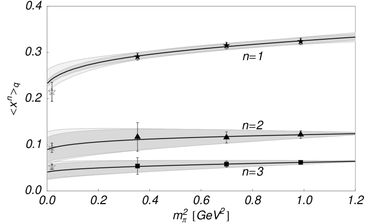
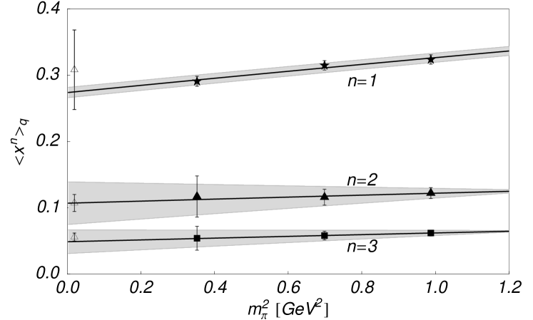
Figure 1: Chiral extrapolation of the lowest three lattice moments Best:1997qp of the pion distributions. The upper plot shows the extrapolation of the valence moments and lower plot shows that of the total moments. The solid curves correspond to fits using Eq. (6), with $\mu=0.7$ GeV for the valence moments, and Eq. (7) for the singlet moments. The dark shaded region in both plots corresponds to fits to the data plus or minus their error bars, while the lighter shaded regions in the valence plot show the additional effect of varying $\mu$ between $0.4$ and $1.0$ GeV on top of the statistical variation. The phenomenological valence (open stars) and total (open triangles) moments are shown at $m_{\pi}^{\rm phys}$ (see Section IV).

The above results for the chiral extrapolation are valid in full QCD, whereas the existing lattice data have been generated within the quenched approximation (in which the effects of background quark loops are neglected). Because quark loop effects are proportional to (powers of) $1/m_{q}$, one expects loops to play a relatively minor role at large quark mass. Indeed, for moments of the nucleon parton distributions the quenched and full QCD simulations were found Dolgov:2002zm to be equivalent within statistical errors for $m_{\pi}\gtrsim 0.5$–0.6 GeV. Therefore, in the present analysis we assume that the available (quenched) data at large $m_{\pi}$ provide a reliable estimate of the unquenched moments at $m_{\pi}\gtrsim 0.5$–0.6 GeV. Future simulations will allow quantitative tests of this assumption, and when they can be performed at quark masses light enough for the difference to become apparent our analysis will need to be repeated using quenched Chen:2001gr (or partially quenched Chen:2001yi ) chiral perturbation theory.

In general the matrix elements receive contributions from diagrams in which the operator insertions are either on quark lines which are connected to the pion source (CI), or on quark lines which are disconnected (DI) (i.e. connected only through gluon lines to the pion source):

$$\langle x^{n}\rangle_{q} = \langle x^{n}\rangle_{q}^{\rm CI}+\langle x^{n}\rangle_{q}^{\rm DI}\ .$$ (9)

The disconnected insertions contribute only to the singlet operators, while the connected diagrams contribute in both the singlet and non-singlet cases. The evaluation of disconnected diagrams is considerably more difficult numerically, and thus far only the connected pieces, $\langle x^{n}\rangle_{q}^{\rm CI}$, have been computed Best:1997qp . Once again we can make use of the large quark masses at which the lattice moments have been simulated by noting that the disconnected insertions should also be suppressed for $m_{\pi}\gtrsim 0.5$ GeV, so that

$$\langle x^{n}\rangle_{q} \approx \langle x^{n}\rangle_{q}^{\rm CI}\ ,\ \ \ \ m_{\pi}\gtrsim 0.5~{}{\rm GeV}\ .$$ (10)

This same argument also suggests that, at these values of $m_{\pi}$, the pion PDFs should satisfy

$$q_{\rm total}(x)\equiv q_{\pi}(x)+\bar{q}_{\pi}(x) \approx q_{\pi}(x)-\bar{q}_{\pi}(x)\ \equiv\ v_{\pi}(x)\ ,$$ (11)

where $v_{\pi}(x)$ is the valence quark distribution in the pion. This observation allows one to approximate the $C$-odd (valence) moments by the $C$-even moments at large $m_{\pi}$, and extrapolate them according to Eq. (6) to compare with the phenomenological valence (non-singlet) moments. However, we stress that future lattice data for the $n$-odd moments should vary smoothly as $m_{q}$ decreases – i.e. they should show no rapid, non-analytic behavior as the chiral limit is approached.

In Fig. 1 we show the lattice data from the QCDSF collaboration Best:1997qp for the $n=1$, 2 and 3 moments (of the $u$ quark distribution in the $\pi^{+}$) as a function of $m_{\pi}^{2}$. The fits to the $n=2$ data using Eq. (6) and those to the $n=1$ and 3 moments using Eq. (7) are indicated by the curves in the upper and lower plots, respectively. For each fit the dark shaded error bands correspond to fits to the data $\pm$ errors. The phenomenological values of the moments, indicated by open stars (valence distribution) and open triangles (total distribution) at $m_{\pi}^{\rm phys}$, are taken from an average of global fits Sutton:1991ay ; Gluck:1999xe to the pion structure function data (see Section IV.1 below). Assuming valence quark dominance of the moments at $m_{\pi}\gtrsim 0.5$ GeV, we also show in the upper plot the $n=1$ and 3 moments extrapolated as if they were non-singlet, using Eq. (6). Under the same assumption we extrapolate the $n=2$ moment as if it were a singlet in the lower plot. In the central curves of the NS fits, we choose $\mu=0.7$ GeV. The outer, lightly-shaded envelopes show a conservative variation of this parameter between 0.4 and 1.0 GeV in addition to the statistical variation (dark shaded region). In all cases the extrapolated moments, both singlet and non-singlet, agree with the phenomenological values within errors, as shown in Table 1. This provides a posteriori evidence for the valence dominance of the moments (suppression of quark loops) at large $m_{\pi}$.

$\langle x^{n}\rangle_{q}$	$n=0$	$n=1$	$n=2$	$n=3$
Moments of Phenomenological PDFs
valence	1	0.21(2)	0.09(1)	0.052(5)
sea [Eq. (15)]	–	0.05(3)	0.007(4)	0.002(1)
total	–	0.31(6)	0.11(1)	0.056(6)
Extrapolated Lattice Moments
valence [method (ii)]	1	0.24(1)(2)	0.09(3)(1)	0.043(15)(3)
valence [method (iii)]	1	0.18(6)	0.10(3)(1)	0.05(2)
sea	–	0.03(1)	–	0.001(9)
total	–	0.275(8)	0.11(3)	0.05(2)

Table 1: Moments of PDFs of the pion, obtained from phenomenological PDFs (see Section IV) and extrapolated from the lattice (as discussed in the text). The $n=2$ lattice total moment is obtained from the lattice valence moment by adding twice the phenomenological sea. The lattice sea is determined by subtracting the phenomenological valence moments from the lattice total moments (for $n$-odd). Errors on the extrapolated lattice moments are calculated from fits to the data $\pm$ their errors (first parentheses) and from varying the parameter $\mu$ between 0.4 and 1.0 GeV (second parentheses, where applicable).

IV Reconstruction of the quark distribution

In this section we use the available lattice moment data to constrain the Bjorken-$x$ dependence of the underlying PDFs. The approach adopted here is similar to that in the earlier analysis of the PDFs in the nucleon Detmold:2001dv ; Detmold:rw ; polrecon . The general procedure is to choose a particular parameterization for the $x$ dependence of the distribution, and perform a Mellin transformation to give the parametric dependence of its moments. Values for the moments, extrapolated from the lattice data, can then used to fit the various parameters and reconstruct the physical distribution.

IV.1 Phenomenological distributions

Before using a specific parameterization to analyze the lattice data, we first test the robustness of the procedure by examining the extent to which the parameters of the phenomenological valence distributions can be reconstructed from their lowest moments. This will provide an estimate of the systematic error in the choice of parameterization and the reconstruction procedure.

Several groups have performed global analyses of pion structure function data and constructed parameterizations of the parton distributions. The valence quark distribution in the SMRS parameterization Sutton:1991ay is fitted with the form

$$v_{\pi}(x)=Ax^{b}(1-x)^{c}\ ,$$ (12)

with the parameters $A$, $b$ and $c$ determined at an input scale of $Q^{2}=4$ GeV², given in Table 2. According to Regge theory, the parameter $b$, which controls the $x\to 0$ behavior, is given by the intercept of the $\rho$ meson trajectory, and is predicted to be $b\approx-1/2$. The parameter $c$ dictates the asymptotic behavior as $x\to 1$, and is predicted by hadron helicity conservation in perturbative QCD to be $c=2$ for the pion Farrar:yb ; Lepage:1980fj ; GUNION . The GRS (next-to-leading order) parameterization Gluck:1999xe contains two additional parameters,

$$v_{\pi}(x)=Ax^{b}(1-x)^{c}(1+e\sqrt{x}+gx)\ ,$$ (13)

with all parameters listed for $Q^{2}=5$ GeV² in Table 2. The small differences in scale between the parameterizations and the lattice moments are negligible.

The phenomenological valence moments with which the lattice calculations are compared are defined by averaging the integrals of these two distributions, and the errors are calculated as the difference between the moments of the two distributions. These average moments are given in Table 1 and shown at the physical pion mass as open stars (valence) and open triangles (total) in Fig. 1.

The Mellin transform of the (more general) parameterization in Eq. (13) is given by

$$\langle x^{n}\rangle_{\rm val} = A\big{[}\beta(1+c,1+b+n)\ +\ e\ \beta(1+c,3/2+b+n)$$ (14)

$$\hskip 28.45274pt+g\ \beta(1+c,2+b+n)\big{]}\ ,$$

where $\beta(a,b)$ is the $\beta$-function. For the simpler SMRS parameterization, only the first term in Eq. (14) is present.

To determine our ability to reconstruct the parameters of a distribution from its moments, we first calculate the moments of the GRS distribution (to be specific) by direct numerical integration. Using Eq. (14), we find that the five parameters in Eq. (14) can be very accurately reconstructed (to 4 significant figures) from the first five moments ($n=0-4$) using a standard Levenberg-Marquardt non-linear fit. However, since only 3 non-trivial lattice moments are currently available, one cannot determine all of the five parameters from the lattice data. If we use the simpler form with $e=g=0$ in Eq. (14) to fit the lowest three non-trivial moments, the parameters $b$ and $c$ that give the best fit to the data differ from those of the underlying distribution by approximately 10% and 30%, respectively. This provides a guide to the size of systematic errors associated with the choice of the parametric form.

IV.2 Valence distribution from lattice moments

Having investigated the accuracy with which one can reliably extract the $x$ dependence of the valence quark distribution from the lowest few moments, we now turn to the extrapolated lattice data discussed in Section III and use these to fit the parameters $A$, $b$ and $c$ in Eq. (12).

There are several possible approaches to reconstructing the $x$ distribution from the available data, which we discuss in the following.

(i) Ideally, the $n$-odd and $n$-even moments should be fitted independently as they correspond to different distributions (Eq. (3)), and the valence distribution extracted from the $n$-even ($C$-odd) lattice moments. In this approach (which we refer to as method (i)), both the statistical and systematic uncertainties (associated with the fact that current lattice data do not constrain $\mu$) of the various extrapolations would be improved by future lattice data. However, the two available ($n=0,2$) moments are not sufficient to constrain all of the parameters in the standard form of Eq. (12). With the existing data, taking $\mu=0.7$ GeV in the extrapolation, the $n=0$ moment fixes $A$, and we find a minimum $\chi^{2}$ along the line $b\approx-0.9+0.2c$ (for $0<c\lesssim 4$). For the case $c=1$, one has $b\approx-0.7$, while for $c=2$, $b\approx-0.5$. Both of these curves are in qualitative agreement with the Drell-Yan data. If it proved feasible to extract the $n=4$ and 6 lattice moments in the future, this method would be ideal.

(ii) An alternative approach is to assume, as discussed in Sec. III, that quark loops are suppressed at large $m_{\pi}$ and that the $n$-odd valence moments are approximately equal to the calculated $C$-even moments in that mass region. This provides us with 4 valence moments to which we fit 3 parameters. We choose $\mu=0.7$ GeV for the central extrapolation, taking $\mu=0.4$ and 1.0 GeV and the lattice data $\pm$ its quoted errors, respectively, as a conservative measure of the overall error. This yields the parameters shown in Table 2 (method (ii)). We determine the uncertainty in the parameters (arising from the statistical errors in the lattice data and the systematic errors in the extrapolation (choice of $\mu$)) by choosing an ensemble of sets of randomly distributed moments within the extrapolated bounds and computing their standard deviation. As discussed above, there is additional systematic uncertainty arising from the reconstruction procedure that is not shown.

The resulting $x$ distribution, which is illustrated in Fig. 2, is in qualitative agreement with the Drell-Yan pion structure function data Conway:fs . At intermediate values of $x$, the extracted distribution tends to lie a little above the experimental data, while at large $x$ it appears to lie slightly below – with an $x\to 1$ behavior similar to that predicted by hadron helicity conservation in perturbative QCD. Of course, given the relatively large errors at present (the shaded region is the envelope of the ensemble of reconstructed distributions used in the error analysis), the distribution shows no significant disagreement with the experimental data.

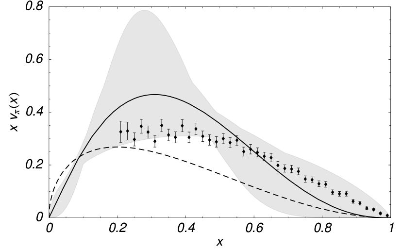
Figure 2: Valence distribution of the pion, reconstructed using method (ii) described in the text. The shaded region corresponds to the uncertainty in the distribution (see text). The dashed line corresponds to $v_{\pi}(x)=Ax^{-1/2}(1-x)^{2}$, which incorporates the hadron helicity conservation expectation for the large-$x$ behavior. Experimental Drell-Yan data (diamonds) are from Ref. Conway:fs .

Since Eq. (6) gives the $m_{\pi}$ dependence of the moments, we can examine the dependence of the valence distribution on the pion mass. The result of reconstructing the PDF at several values of $m_{\pi}^{2}$ is shown in Fig. 3. We do not show results for values of $m_{\pi}^{2}$ larger than 1 GeV² because there are no lattice data to constrain the reconstruction. However, we have checked that if the heavy quark limit is built into our extrapolation function, the distribution approaches a $\delta$-function at $x=1/2$. It is interesting that, even without such a constraint, the PDF seems to show that the momentum of the pion is shared primarily between the two valence quarks for $m_{\pi}$ above 0.7 GeV.

Figure 3: Mass dependence of the valence quark distribution of the pion (with $m_{\pi}$ in GeV).

The obvious problem with this method is that the assumption that the $C$-odd and $C$-even moments are approximately equal must break down as the lattice data are extended to lower masses — presumably where one begins to see curvature in the $n=2$ moment.

(iii) A third possibility is to extrapolate the $n$-odd moments linearly, according to Eq. (7), and subtract twice the moments of the phenomenological sea at the physical mass to give the valence moments. The disadvantage of this method is that it relies on phenomenological information in addition to that obtained from the lattice. Moreover, the sea quark distribution in the pion is only very weakly constrained by experimental data, so that the errors on the valence, $n$-odd moments will be large compared to those on the $n$-odd total moments extracted from the lattice. A further disadvantage of this method, from the purely theoretical point of view, is that in this approach one obviously cannot study the variation of the pion PDFs as a function of quark mass, as was done for method (ii) above and for the nucleon in Ref. Detmold:2001dv . On the other hand, the errors on the extrapolations can be improved systematically as the lattice data at smaller quark masses become available and new experiments better constrain the pion sea JLAB12 ; HERA .

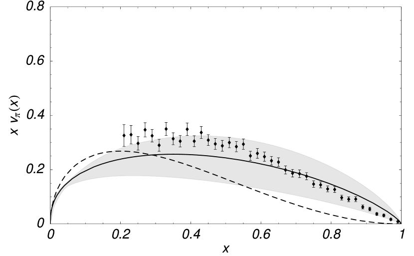
Figure 4: As in Fig. 2, but using method (iii) to reconstruct the valence pion distribution.

Taking the $n$-odd sea moments from an average of the SMRS and GRS distributions and extrapolating the $n=2$ moment with $\mu=0.7$ GeV gives the parameters shown in Table 2 as method (iii). Errors are as described for method (ii) (where relevant). These parameters yield a distribution which is in good agreement with the Drell-Yan data, as seen in Fig. 4. In particular, the extracted curves are consistent with (though slightly harder than) the $x\to 1$ behavior found in the experimental analyses, which, however, disagree with the hadron helicity conservation predictions.

While there is some difference between the detailed $x$ dependence for the valence quark distribution obtained using the methods (ii) and (iii), these should disappear once more accurate lattice data on the moments become available. Nevertheless, the fact that both methods are in reasonable agreement with the Drell-Yan data, and with each other, is very encouraging. It would be particularly valuable to have accurate higher moments ($n=4$–6) in order to constrain the detailed shape of the distribution.

Fit	$A$	$b$	$c$
SMRS	1.08	–0.36	1.08
GRS	0.98	–0.47	1.02
method (ii)	4.4	0.1(5)	2.5(1.5)
method (iii)	0.6	–0.6(3)	0.8(9)

Table 2: Parameters of the valence distributions from various methods of analysis. The GRS valence distribution (13) in addition uses the parameters $e=-0.81$ and $g=0.64$. The quoted errors combine the statistical and systematic (from $\mu$) errors. (Note that the lower limit on the parameter $c$ for method (iii) is constrained to be positive.) Errors are not given for $A$ as it is constrained by normalization. There is some additional systematic uncertainty from the reconstruction procedure which is not shown but is discussed in the text.

IV.3 Sea distribution

The sea quark distribution in the pion, defined as

$$s_{\pi}(x) \equiv {1\over 2}(q_{\pi}(x)-v_{\pi}(x))\ ,$$ (15)

is relatively poorly known experimentally. There are no data from the Drell-Yan reaction for $x\lesssim 0.2$ Betev:1985pg ; Conway:fs , and the size of the sea is constrained only by imposing the momentum sum rule. A simple parameterization of the pion sea (as used by SMRS Sutton:1991ay ) is

$$x\ s_{\pi}(x)=A_{s}(1-x)^{\eta}\ .$$ (16)

The analysis of GRS Gluck:1999xe determines the pion sea with reference to the proton sea. A similar constraint can be derived at $x\sim 10^{-2}$ from semi-inclusive DIS measurements at HERA, with the result $F_{2}^{\pi}\approx F_{2}^{N}/3$ HERA . This finding tends to favor the SMRS sea over that of GRS Klasen:2001dd , however, this information corresponds to such small values of $x$ that it is of little assistance for the present analysis.

In order to obtain information on the pion sea from the lattice data, one would ideally extract the valence distribution according to method (i) above, and use this to calculate the $n$-odd valence moments. These would then be subtracted from the total moments, obtained from the corresponding extrapolation of the lattice data to obtain the $n$-odd moments of the pion sea at the physical pion mass. The $x$ dependence of the sea distribution could then be reconstructed using the form (16), given enough moments.

In the absence of sufficiently many moments for this to be a practical solution, an alternative is to use the phenomenological valence ($n$-odd) moments instead of the lattice moments. Since these moments are relatively well known, this procedure should be reasonably reliable. The $n$-odd sea moments which we extract using the linearly extrapolated total moments from the lattice minus the phenomenological valence moments are given in Table 1. Using these data to fit the Mellin transform of Eq. (16), we find the parameters $A_{s}=0.27$ and $\eta=5.8$. Unfortunately, the statistical uncertainty in these lattice sea moments is large and the constraints on these parameters are very weak. In particular, the third moment of the sea is consistent with zero: for $\langle x^{3}\rangle_{\rm sea}\to 0$ the reconstruction gives $\eta\to\infty$. Nevertheless, this is in principle improvable and if the size of the errors on the $n=3$ lattice moment were comparable to that on the $n=1$ moment, a more robust reconstruction could be performed.

One could also modify this method by including the $n=2$ sea moment constructed from the difference of the linear and chiral extrapolations of the lattice data. However, this introduces additional uncertainty (from $\mu$) in the analysis and does not reduce the uncertainty in the reconstructions.

V Summary and prospects

We have studied the problem of the chiral extrapolation of the moments of the PDFs of the pion, from the large quark masses where current lattice QCD calculations are performed to the physical values. As in earlier studies of the PDFs of the nucleon, the non-linearity of the model independent non-analytic variation of the moments of the valence PDF is extremely important, producing a significant change in the moments at the physical quark mass, compared with a naive linear extrapolation. In comparison, the moments of the singlet distribution, $q+\bar{q}$, show no non-analytic behavior and are therefore expected to extrapolate smoothly to the chiral limit.

Having studied the extrapolation of the moments of both the singlet and non-singlet PDFs, we examine various procedures for reconstructing the valence and sea distributions of the pion from the lattice moments. To make optimal use of the available lattice data for the $n=1$–3 moments, we make the reasonable assumption that at large quark masses ($m_{\pi}\gtrsim 500$–600 MeV) the effects of quark loops are suppressed, so that the effects of the quenched approximation and disconnected insertions will not affect the extrapolation. This allows the parameters of the valence, and to some extent the sea, quark distributions to be determined, and the extracted distribution compared with the available Drell-Yan data. Over the range of intermediate $x$, from 0.2 to 0.8, the reconstructed valence distribution is in fair agreement with the Drell-Yan data, within the rather large errors arising from the extrapolation procedure. At this stage, however, it is not possible to distinguish between the large-$x$ behavior predicted from hadron helicity conservation in perturbative QCD and that found in the Drell-Yan data. Nevertheless, new lattice simulations, on the much faster computers expected to be devoted to lattice QCD in the next few years, should offer the chance, when analyzed using the techniques set out here, to determine leading twist PDFs with an accuracy that exceeds that of current experiments.

The results of this analysis can be used to guide future studies of PDFs in lattice gauge theory. Specifically,

• The clearest observation is that it would be extremely valuable to have quenched calculations for the $n=2$ and $n=3$ moments of an accuracy comparable to that for $n=1$. This is especially important for pion masses below 0.4 GeV². This alone would make a substantial improvement in the errors on the parton distribution functions. To better constrain the functional form of the $x$-dependence, calculations of several higher moments (e.g. $n=4,5$) would also be desirable.

• In the case of the nucleon there is no observable difference between the moments calculated in quenched and full QCD in the mass range covered. It is vital to check that this is also true for the pion.

• In order to better constrain the extrapolation and to assure us that we are on the right track it is important to push the lattice simulations to lower pion masses. Ideally this should occur in full (unquenched) QCD; however, quenched, and especially partially-quenched (which is a computationally efficient way to get to smaller valence quark mass without actually ignoring quark loops) simulations would also provide valuable information to guide the chiral extrapolation.

• Of course, if one wants to explore the sea quark distribution, for which there is little hard information at present, it will also be necessary to include disconnected quark loops, even though it is difficult to pick out a signal for such terms Lewis:2002tz .

• Finally, as with all lattice simulations, we need to confirm that the continuum ($a\rightarrow 0$) and infinite volume ($L\rightarrow\infty$) corrections are fully under control.

With such a program we could expect significant advances over the next few years in our understanding of the quark structure of the pion in QCD.

- (1) J. Badier et al. [NA3 Collaboration], Z. Phys. C 18, 281 (1983).
- (2) B. Betev et al. [NA10 Collaboration], Z. Phys. C 28, 15 (1985).
- (3) P. Aurenche, R. Baier, M. Fontannaz, M. N. Kienzle-Focacci and M. Werlen, Phys. Lett. B 233, 517 (1989).
- (4) M. Bonesini et al. [WA70 Collaboration], Z. Phys. C 37, 535 (1988).
- (5) J. S. Conway et al., Phys. Rev. D 39, 92 (1989).
- (6) M. Klasen, J. Phys. G 28, 1091 (2002).
- (7) H. Holtmann, G. Levman, N. N. Nikolaev, A. Szczurek and J. Speth, Phys. Lett. B 338, 363 (1994).
- (8) G. Levman, in Lepton Scattering, Hadrons and QCD, eds. W. Melnitchouk et al. (World Scientific, 2001); Nucl. Phys. B642, 3 (2002).
- (9) R. J. Holt, P. E. Reimer and K. Wijesooriya, Jefferson Lab Proposal PR-01-110 (2001); in Hall A Preliminary Conceptual Design Report for the Jefferson Lab 12 GeV Upgrade (2002).
- (10) J. F. Owens, Phys. Rev. D 30, 943 (1984).
- (11) P. J. Sutton, A. D. Martin, R. G. Roberts and W. J. Stirling, Phys. Rev. D 45, 2349 (1992).
- (12) M. Gluck, E. Reya and I. Schienbein, Eur. Phys. J. C 10, 313 (1999).
- (13) M. Gluck, E. Reya and A. Vogt, Z. Phys. C 53, 651 (1992).
- (14) M. Gluck, E. Reya and M. Stratmann, Eur. Phys. J. C 2, 159 (1998).
- (15) G. Altarelli, S. Petrarca and F. Rapuano, Phys. Lett. B 373, 200 (1996).
- (16) W. Bentz, T. Hama, T. Matsuki and K. Yazaki, Nucl. Phys. A651, 143 (1999).
- (17) T. Shigetani, K. Suzuki and H. Toki, Phys. Lett. B 308, 383 (1993).
- (18) R. M. Davidson and E. Ruiz Arriola, Acta Phys. Polon. B 33, 1791 (2002).
- (19) E. Ruiz Arriola and W. Broniowski, Phys. Rev. D 66, 094016 (2002).
- (20) A. E. Dorokhov and L. Tomio, Phys. Rev. D 62, 014016 (2000).
- (21) F. Bissey, J. R. Cudell, J. Cugnon, M. Jaminon, J. P. Lansberg and P. Stassart, Phys. Lett. B 547, 210 (2002).
- (22) T. Frederico and G. A. Miller, Phys. Rev. D 50, 210 (1994).
- (23) W. Melnitchouk, hep-ph/0208258.
- (24) M. B. Hecht, C. D. Roberts and S. M. Schmidt, Phys. Rev. C 63, 025213 (2001).
- (25) G. R. Farrar and D. R. Jackson, Phys. Rev. Lett. 35, 1416 (1975).
- (26) G. R. Farrar and D. R. Jackson, Phys. Rev. Lett. 43, 246 (1979).
- (27) G. P. Lepage and S. J. Brodsky, Phys. Rev. D 22, 2157 (1980).
- (28) J. F. Gunion, P. Nason and R. Blankenbecler, Phys. Rev. D 29, 2491 (1984).
- (29) E. L. Berger and S. J. Brodsky, Phys. Rev. Lett. 42, 940 (1979).
- (30) G. Martinelli and C. T. Sachrajda, Nucl. Phys. B306, 865 (1988).
- (31) G. Martinelli and C. T. Sachrajda, Phys. Lett. B 196, 184 (1987).
- (32) J. T. Londergan and A. W. Thomas, Prog. Part. Nucl. Phys. 41, 49 (1998).
- (33) J. T. Londergan, G. Q. Liu, E. N. Rodionov and A. W. Thomas, Phys. Lett. B 361, 110 (1995).
- (34) C. Best et al., Phys. Rev. D 56, 2743 (1997).
- (35) D. B. Leinweber, A. W. Thomas, K. Tsushima and S. V. Wright, Phys. Rev. D 64, 094502 (2001).
- (36) S. Capitani et al., Nucl. Phys. B570, 393 (2000).
- (37) W. Detmold, W. Melnitchouk, J. W. Negele, D. B. Renner and A. W. Thomas, Phys. Rev. Lett. 87, 172001 (2001).
- (38) D. Dolgov et al. [LHP Collaboration], Phys. Rev. D 66, 034506 (2002).
- (39) K. Jansen, hep-lat/0010038.
- (40) S. R. Sharpe, Phys. Rev. D 56, 7052 (1997) [Erratum-ibid. D 62, 099901 (2000)].
- (41) S. Weinberg, Physica (Amsterdam) 96 A, 327 (1079); J. Gasser and H. Leutweyler, Ann. Phys. 158, 142 (1984).
- (42) A. W. Thomas, W. Melnitchouk and F. M. Steffens, Phys. Rev. Lett. 85, 2892 (2000).
- (43) W. Detmold, W. Melnitchouk and A. W. Thomas, Eur. Phys. J. directC 3, 13 (2001).
- (44) W. Detmold, Nucl. Phys. Proc. Suppl. 109A, 40 (2002).
- (45) W. Detmold, W. Melnitchouk and A.W. Thomas, talk given at the 3rd Circum-Pan-Pacific Symposium on High Energy Spin Physics, Beijing, China (2001), to appear in Int. J. Mod. Phys. A, hep-ph/0201288.
- (46) W. Detmold, W. Melnitchouk and A. W. Thomas, Phys. Rev. D 66, 054501 (2002).
- (47) D. Arndt and M. J. Savage, Nucl. Phys. A697, 429 (2002).
- (48) J. W. Chen and X. Ji, Phys. Lett. B 523, 107 (2001).
- (49) A. W. Thomas, in Proceedings of 20th International Symposium on Lattice Field Theory, Boston, Massachusetts, 2002, hep-lat/0208023.
- (50) J. W. Chen and M. J. Savage, Nucl. Phys. A707, 452 (2002).
- (51) J. W. Chen and M. J. Savage, Phys. Rev. D 65, 094001 (2002).
- (52) M. Göckeler et al., in Physics with polarized protons at HERA, eds. J. Blumlein et al. (DESY, Zeuthen, 1997), hep-ph/9711245.
- (53) G. Levman, J. Phys. G 28, 1079 (2002).
- (54) R. Lewis, W. Wilcox and R. M. Woloshyn, arXiv:hep-ph/0201190.