DESY/03-028 SFB/CPP-4 March 2003
Continuous external momenta in
non-perturbative lattice simulations:
a computation of renormalization factors

We discuss the usage of continuous external momenta for computing renormalization factors as needed to renormalize operator matrix elements. These kind of external momenta are encoded in special boundary conditions for the fermion fields. The method allows to compute certain renormalization factors on the lattice that would have been very difficult, if not impossible, to compute with standard methods. As a result we give the renormalization group invariant step scaling function for a twist-2 operator corresponding to the average momentum of non-singlet quark densities.

1 Introduction

One of the most important contributions lattice gauge theory can provide to test QCD and to interpret experimental data, is the computation of non-perturbatively renormalized matrix elements. The example we are interested in here are matrix elements that are connected to moments of parton distribution functions as can be extracted from global fits to experimental data in deep inelastic scattering. The matrix elements are related themselves to certain operator expectation values which are accessible from lattice simulations.

When considering operators that contain derivatives, a saturation with external momenta is needed to perform the necessary contractions. This applies for computing the renormalization constants as well as matrix elements of such operators. On an euclidean lattice, the standard momenta are quantized in units of $2\pi a/L$ with $a$ the lattice spacing and $L$ the linear extent of a lattice of physical size $L^{4}$. Unfortunately, the introduction of a momentum in a numerical simulation leads often to either large lattice artefacts or to large statistical uncertainties or to both such that reliable measurements of such quantities become difficult.

In this paper we will demonstrate how the introduction of special boundary conditions of the fermion fields, first advocated in [1], can help in such a situation. The boundary conditions lead to continuous values of external momenta $a\theta/L$ where $\theta$ varies continuously in the range $0\leq\theta\leq 2\pi$ giving a large flexibility of a momentum definition in lattice simulations. In particular, the minimal value of a lattice momentum can be chosen smaller than in the standard set-up which might lead to smaller lattice artefacts. As we will see in the example discussed below, the use of these kind of continuous external momenta will allow us to compute renormalization constants reliably on the lattice for which measurements were very difficult in the standard set-up. It might be, however, that the method is much more general and goes beyond the application investigated here.

The physical example we will discuss in this paper is the calculation of renormalization constants as needed for twist-2, non-singlet quark operators in the framework of computing moments of parton distribution functions in deep inelastic scattering. The interest in this calculation is twofold. First, we want to demonstrate the feasibility of using continuous momenta in a lattice computation.

Second, the success of this demonstration will allow us to correct a small mismatch of our earlier work: In a series of papers [2, 3, 4, 5, 6] we have demonstrated that the Schrödinger functional (SF) formalism [7] can be used to compute non-perturbatively moments of parton distribution functions (for summaries of the results, see [8, 9, 10]). A problem that arises naturally in lattice computations of such quantities is that for a given continuum operator there is not a unique representation of that operator on the lattice. In fact, in the old work cited above, the operator used to compute the matrix element and the operator used to compute the corresponding renormalization constant were in two different representations. Although in ref. [6] we argued that this mismatch only leads to a small, negligible error, the situation remains rather unsatisfactory, as we want a fully non-perturbative way to evaluate the physical matrix element without systematic uncertainties. The usage of the continuous external momenta will allow us to eliminate this small systematic uncertainty. In particular, we will show that we can compute the scale dependent renormalization constant and the corresponding (ultra-violet) invariant step scaling function for a particular lattice representation which is needed to perform the correct renormalization for the physical matrix element. In this way, we will be able to provide a non-perturbative lattice computation of the average momentum carried by the quarks in a hadron.

2 Basic definitions and choice of boundary conditions

A bare, local operator $\mathcal{O}^{\mathrm{bare}}$ as considered here, is renormalized multiplicatively by a scale $\mu$ dependent renormalization constant $Z_{{\cal O}}(\mu)$. The renormalized operator ${\cal O}^{R}(\mu)$ is then given by

$${\cal O}^{R}(\mu)=Z_{{\cal O}}^{-1}(\mu){\cal O}^{\rm bare}\;.$$ (1)

The evolution of ${\cal O}$ from a renormalization scale $\mu_{1}$ to $\mu_{2}$ is described by the continuum step scaling function $\sigma_{Z_{{\cal O}}}$ that can formally be written as

$$\sigma_{Z_{{\cal O}}}(\mu_{1}/\mu_{2})=\frac{Z_{{\cal O}}(\mu_{2})}{Z_{{\cal O}}(\mu_{1})}\;.$$ (2)

The individual $Z$’s in eq. (2) are only well-defined within a given regularization scheme and would be divergent when the regularization is removed. The step scaling function, however, is a well-defined quantity even in this limit. In the following we will give a rigorous definition of the renormalization constants and of the step scaling function using the lattice regularization in the Schrödinger functional (SF) scheme.

The SF scheme is based on the formulation of QCD in a finite space-time volume of size $L^{3}\cdot T$. In this paper we will always use $L=T$. In this scheme a change of renormalization scale amounts to a change of the box size $L$ at fixed bare parameters. By considering a sequence of pairs of volumes with sizes $L$ and $sL$, one can study the evolution of a given local operator under repeated changes of the scale by a factor of $s$. Effectively in this way one builds up a non-perturbative renormalization group. To be specific, we will from now on work on a euclidean lattice as regulator.

The fermion and gauge fields on the lattice are defined in the standard way, fulfilling SF boundary conditions, as detailed in ref. [7]. Besides these special boundary conditions in time direction, we will impose generalized boundary conditions in the spatial directions (denoted by $\hat{k}$) for the fermion fields $\psi(x)$ [1]

$$\psi(x+L\hat{k})=e^{i\theta_{k}}\psi(x),\;\;\bar{\psi}(x+L\hat{k})=e^{-i\theta_{k}}\bar{\psi}(x),\;k=1,\;2,\;3,$$ (3)

while the gauge fields $U(x,k)$ are chosen to be periodic in the space directions. The values of $\theta_{k}$ can be chosen in the interval $0\leq\theta_{k}\leq 2\pi$. For $\theta_{k}=0$ we obtain periodic and for $\theta_{k}=\pi$ we get anti-periodic boundary conditions.

The generalized boundary conditions of eq. (3) can be implemented in the definition of the gauge covariant lattice derivatives:

$$\nabla_{\mu}\psi(x) = \frac{1}{a}\left[\lambda_{\mu}U(x,\mu)\psi(x+a\hat{\mu})-\psi(x)\right]$$

$$\nabla_{\mu}^{*}\psi(x) = \frac{1}{a}\left[\psi(x)-\lambda_{\mu}^{*}U(x-a\hat{\mu},\mu)\psi(x-a\hat{\mu})\right]$$ (4)

with $\mu=(k,4)$,

$$\lambda_{\mu}=e^{ia\theta_{\mu}/L},\;\;0\leq\theta_{k}\leq 2\pi,\;\;\theta_{4}=0,$$ (5)

and $a$ the lattice spacing. From a technical point of view the fields $\psi(x)$ and $\bar{\psi}(x)$ are then implemented with the usual periodic boundary conditions in the space directions utilizing this generalized definition of the covariant derivative of eq. (4).

The crucial observation [1] is that the factor $e^{ia\theta_{k}/L}$ can be interpreted as an external momentum with the intriguing property that it can assume continuous values, in contrast to the standard, quantized lattice momenta that assumes values in units of $2\pi a/L$ only.

In order to explore the flexibility of a momentum definition given by the generalized boundary conditions in eq. (3) we have concentrated in this work on the twist-2, non-singlet (quark) operator. This amounts to consider operators of the form (the flavor structure is specified by the Pauli matrix $\tau^{3}$)

$${\mathcal{O}}_{\mu\nu}(x)=\frac{1}{4}\bar{\psi}(x)\gamma_{\{\mu}\stackrel{{\scriptstyle\leftrightarrow}}{{D}}_{\nu\}}\frac{1}{2}\tau^{3}\psi(x)-\delta_{\mu\nu}\cdot{\rm trace~{}terms}\;.$$ (6)

where $\{\cdots\}$ means symmetrization on the Lorentz indices and

$$\stackrel{{\scriptstyle\leftrightarrow}}{{D}}_{\mu}=\stackrel{{\scriptstyle\rightarrow}}{{D}}_{\mu}-\stackrel{{\scriptstyle\leftarrow}}{{D}}_{\mu};\qquad D_{\mu}=\frac{1}{2}[\nabla_{\mu}+\nabla_{\mu}^{*}]\;.$$ (7)

There are two representations of such a non-singlet operator on the lattice [11]. The first representation takes $\mu\neq\nu$ whereas the second uses $\mu=\nu$. The precise definitions of the operators used here are

$${\cal O}_{12}(x)=\frac{1}{4}\bar{\psi}(x)\gamma_{\{1}\stackrel{{\scriptstyle\leftrightarrow}}{{D}}_{2\}}\frac{1}{2}\tau^{3}\psi(x)$$ (8)

and

$${\cal O}_{44}(x)=\frac{1}{2}\bar{\psi}(x)\Big{[}\gamma_{4}\stackrel{{\scriptstyle\leftrightarrow}}{{D}}_{4}-\frac{1}{3}\sum_{k=1}^{3}\gamma_{k}\stackrel{{\scriptstyle\leftrightarrow}}{{D}}_{k}\Big{]}\frac{\tau^{3}}{2}\psi(x)\;.$$ (9)

In both cases an external momentum has to be supplied to compute their renormalization constants. We will realize these momenta with non-vanishing values of $\theta_{k}$, implicitly given through the covariant derivatives in the fermion action and the operators in eqs. (8), (9). The precise choice we adopt here is

$$\theta\equiv\theta_{1}\neq 0,\;\theta_{2}=\theta_{3}=0\;.$$ (10)

In order to make the discussion in the following self-consistent, let us recall the definition of bare correlation functions in the SF scheme [3] as needed to compute appropriate renormalization factors. The correlation function of a given operator ${\cal O}$ is given by

$$f_{\cal O}(x_{4}/L,\theta)=-{a^{6}\over{L^{3}}}\sum_{\bf x,y,z}\langle{\cal O}_{\mu\nu}(x)\ \bar{\zeta}({\bf y})\Gamma\frac{1}{2}\tau^{3}\zeta({\bf z})\rangle\;,$$ (11)

where $\Gamma$ is a Dirac matrix that in our case is $\gamma_{2}$ for the ${\cal O}_{12}$ operator, while it is $\gamma_{1}$ for ${\cal O}_{44}$. In eq. (11) $\zeta$ and $\bar{\zeta}$ are classical boundary fields at $x_{4}=0$ and we sum over space. In order to normalize such correlation functions properly, we also need the “boundary to boundary” correlation function $f_{1}$,

$$f_{1}(\theta)=-{{a^{12}}\over{L^{6}}}\sum_{\bf u,v,y,z}\langle\bar{\zeta}^{\prime}({\bf u})\gamma_{5}\frac{1}{2}\tau^{a}\zeta^{\prime}({\bf v})\bar{\zeta}({\bf y})\gamma_{5}\frac{1}{2}\tau^{a}\zeta({\bf z})\rangle\;.$$ (12)

Note that the classical boundary source fields $\zeta,\bar{\zeta}$ at $x_{4}=0$ and $\zeta^{\prime},\bar{\zeta}^{\prime}$ at $x_{4}=L$ are renormalized multiplicatively with a common renormalization constant $Z_{\zeta}$ [12, 13]. The momentum ($\theta$) dependence of the correlation functions $f_{{\cal O}}$ in eq. (11) and $f_{1}$ in eq. (12) is again implicitly given through the definition of the covariant derivative eq. (4) that appears in the fermion action and in the operator considered.

It is instructive to look at the $\theta$-dependence of the correlation functions $f_{{\cal O}_{44}}$ and $f_{{\cal O}_{12}}$ for fixed values of $x_{4}/L=1/2$ and $x_{4}/L=1/4$ already at tree-level.

Figure 1: $\theta$-dependence of $f_{{\cal O}}$ at tree-level. For the ${\cal O}_{44}$ representation the tree-level values at $x_{4}=L/2$ and $x_{4}=L/4$ are the same.

Fig. 1 shows the tree-level correlation functions $f_{{\cal O}}^{(0)}$. It can be observed that the signal strongly depends on the chosen value of $\theta$, the definition of the operator and the choice of $x_{4}/L$. For small values of $\theta$ all correlation functions show a linear behavior in $\theta$ and vanish at $\theta=0$. In contrast to the correlation function of the operator ${\cal O}_{12}$, the correlator for ${\cal O}_{44}$, which does not depend on $x_{4}/L$ at tree-level, becomes very small for values of, say, $\theta>4.5$, see the inlay in fig. 1. This implies that for a real simulation there is a danger that for these $\theta$-values the signal may become very small, too. In addition, it seems that for these values of $\theta$, due to large lattice artifacts (cf. sect. 2.2) it may become hard to extract even the one-loop anomalous dimension. It should be concluded therefore that the choice of $\theta$ in a simulation needs an optimization procedure. Before we can start a discussion of how to perform this optimization we first want to give here the renormalization conditions we have used in order to determine the renormalization factors which are defined as follows.

 

$${Z_{{\cal O}}(a/L,x_{4}/L,\theta,\theta^{\prime})~{}}$$

  (13)

where the correlation functions are being evaluated at vanishing quark mass $m_{\rm q}=0$ and for vanishing boundary gauge and fermion fields. The renormalization conditions are chosen such that $Z_{{\cal O}}=1~{}{\rm{and}}~{}{\bar{Z}}_{{\cal O}}=1$ at tree-level of perturbation theory at a fixed scale $\mu=1/L$ [2, 3] while the external parameters $\theta$, $\theta^{\prime}$ and $x_{4}/L$ can be varied. From these conditions we obtain

 

$${c=\frac{\sqrt{f_{1}^{(0)}}}{f_{\cal O}^{(0)}}\;,\;\;\bar{c}=\frac{1}{f_{\cal O}^{(0)}}\;.}$$

  (14)

The quantities $c~{}{\rm{and}}~{}\bar{c}$ are the expressions of the correlation functions in eq. (11) and in eq. (12) at tree-level with the corresponding arguments. Note that the actual renormalization constant needed is $Z_{\cal O}$ whereas ${\bar{Z}}_{\cal O}$ is only an auxiliary quantity that, however, proved useful in our previous work [3]. Note that in the definition of the renormalization constants in eq. (13) we leave the freedom to choose $\theta\neq\theta^{\prime}$ for $f_{\cal O}$ and $f_{1}$. It is important to stress here that a different choice of $x_{4}/L$, $\theta$ and $\theta^{\prime}$ defines a different renormalization scheme. In this paper we have considered two families of renormalization schemes,

• scheme A $\qquad\qquad\theta^{\prime}=\theta$

• scheme B $\qquad\qquad\theta^{\prime}=0$  .

Both schemes are studied in the following with respect to analyzing the convergence of perturbation theory, the size of cutoff effects and the signal to noise ratio. In these studies the external parameters $\theta$ and $x_{4}/L$ are tuned to optimize these criteria.

2.1 Convergence of perturbation theory

In this section we present a perturbative analysis of renormalization constants for the local operators in eq. (8) and in eq. (9). In particular we compute the 2-loop anomalous dimension for the Z-factors for the two schemes discussed above. In bare perturbation theory the renormalization constants have an expansion of the form

$$Z_{{\cal O}}(g_{0},a/L,x_{4}/L,\theta)=1+\sum_{k=1}^{\infty}Z_{{\cal O}}^{(k)}(a/L,x_{4}/L,\theta)\,g_{0}^{2k},$$ (15)

where in the limit $a/L\to 0$ the coefficients $Z_{{\cal O}}^{(k)}$ are polynomials in $\ln(L/a)$ of degree $k$ up to corrections of O($a/L$). In particular the coefficient of the logarithmic divergence in $Z_{{\cal O}}^{(1)}$ is given by the one-loop anomalous dimension $\gamma_{0}$, and thus $Z_{{\cal O}}^{(1)}$ is parameterized as

$$Z_{{\cal O}}^{(1)}=B_{\cal O}(\theta,x_{4}/L)-\gamma_{0}\ln(L/a)+{\rm O}(a/L)\;.$$ (16)

The values for the 1-loop anomalous dimension $\gamma_{0}$ and the constant piece $B_{\cal O}(\theta,x_{4}/L)$ can be computed in lattice perturbation theory for the SF scheme following the techniques developed in [2, 14]. For the matching of the non-perturbative lattice results and perturbation theory at very high energies, it is important to know also the 2-loop anomalous dimension $\gamma_{1}$. Since $\gamma_{1}$ is not universal, it becomes necessary to compute the dependence of $\gamma_{1}$ on the values of $\theta$ and $x_{4}/L$. In this way it becomes possible to control for which choice of these parameters $\gamma_{1}/\gamma_{0}$ is small in order to have a good behavior of the perturbative series.

The coefficient $Z_{\cal O}^{(2)}\propto\gamma_{1}\ln(L/a)$ can actually be obtained without an explicit 2-loop calculation in the SF scheme if the 2-loop anomalous dimension is already known from a different renormalization scheme [15]. The formula relating the 2-loop anomalous dimensions in the SF and the $\overline{\mathrm{MS}}$ schemes is given by

$$\gamma_{1}=\gamma_{1}^{\overline{\mathrm{MS}}}+2b_{0}\Delta Z_{{\cal O}}^{(1)}-\gamma_{0}{\cal X}_{\rm g}^{(1)}\;.$$ (17)

In eq. (17) $b_{0}$ is the universal 1-loop coefficient of the $\beta$-function, $\Delta Z_{{\cal O}}^{(1)}$ is the 1-loop difference of the renormalization constants from a finite renormalization that relates two mass-independent schemes and ${\cal X}_{\rm g}^{(1)}$ is the perturbative factor that relates the renormalized couplings in the two schemes considered (see the appendix for explicit expressions of these quantities).

A subtlety is that the factor $\Delta Z_{{\cal O}}^{(1)}$ needs to be computed in two different regularizations, in order to avoid a calculation with the SF scheme using a dimensional regularization (DR).

Figure 2: Graphical representation of the finite renormalization between schemes when a different regularization is used.

Let us explain this fact. A matrix element ${\cal O}_{R}^{s}$ renormalized in a certain scheme $s$ is obtained by

$${\cal O}_{R}^{s}=Z_{{\cal O}}^{s,reg}{\cal O}_{b}^{reg}$$ (18)

where ${\cal O}_{b}^{reg}$ is the bare matrix element computed within a certain regularization $reg$ and $Z_{{\cal O}}^{s,reg}$ is the renormalization constant that depends on the renormalization scheme $s$ used and on the regularization $reg$. Operators renormalized in two different schemes but using the same regularization can be related by a finite renormalization

$${\cal O}^{s^{\prime}}={\cal O}^{s}\Delta Z_{{\cal O}}^{s^{\prime}\leftarrow s}\;.$$ (19)

One important observation here is that $\Delta Z_{{\cal O}}^{s^{\prime}\leftarrow s}$ is independent from the regularization used to compute the renormalized matrix element and the corresponding renormalization constant. This allows to relate two schemes: in principle it is possible to compute the complete 1-loop renormalization constant (anomalous dimension and finite part) in the SF scheme, using the dimensional regularization and then connect directly with the $\overline{\mathrm{MS}}$ scheme (dashed line in fig. 2),

$$\Delta Z_{{\cal O}}^{SF\leftarrow\overline{\mathrm{MS}}}=Z_{{\cal O}}^{SF,DR}/Z_{{\cal O}}^{\overline{\mathrm{MS}},DR}\;.$$ (20)

A lattice perturbative computation will give, on the other side, important information about the amount of discretization errors at 1-loop and would help the numerical calculation. In order to avoid an additional computation in the SF scheme one may now use the MOM scheme, where a complete 1-loop computation has been done for the renormalization constant in both regularization schemes [16].

The desired factor $\Delta Z_{{\cal O}}^{SF\leftarrow\overline{\mathrm{MS}}}$ relating the SF to the $\overline{\mathrm{MS}}$ scheme (full line in fig. 2) can now be obtained from

$$\Delta Z_{{\cal O}}^{SF\leftarrow\overline{\mathrm{MS}}}=\Delta Z_{{\cal O}}^{SF\leftarrow MOM}\Delta Z_{{\cal O}}^{MOM\leftarrow\overline{\mathrm{MS}}}\;.$$ (21)

The two factors $\Delta Z$ are computed using different regularizations, namely $\Delta Z_{{\cal O}}^{SF\leftarrow MOM}$ is computed on the lattice and $\Delta Z_{{\cal O}}^{MOM\leftarrow\overline{\mathrm{MS}}}$ in dimensional regularization. Using the complete one loop result [16] in the MOM scheme which exists in both, lattice and dimensional, regularizations, it is then possible to compute $\Delta Z_{{\cal O}}^{(1)}$ and from this finally $\gamma_{1}$.

In table 1 we give values for $\gamma_{1}$ for selected values of $\theta$ and $x_{4}/L=1/2$. From this table we observe that the ratio $\gamma_{1}/\gamma_{0}$ becomes smaller for increasing values of $\theta$ if we choose the scheme A ($\theta=\theta^{\prime}$). For scheme B ($\theta^{\prime}=0$), we find a kind of minimum of this ratio for $\theta\approx 1.6$. We repeated the analysis for the anomalous dimensions for $x_{4}/L=1/4$ and found a very similar pattern. Thus we have a first indication for the choice of $\theta$ to be chosen.

$\theta$	$\gamma^{A}_{1}(\theta)$	$\gamma^{B}_{1}(\theta)$	$\gamma^{A}_{1}(\theta)/\gamma_{0}$	$\gamma^{B}_{1}(\theta)/\gamma_{0}$
$0.1$	$\phantom{-}0.06584(1)$	$\phantom{-}0.06551(1)$	$\phantom{-}1.4621(6)$	$\phantom{-}1.4548(3)$
$0.4$	$\phantom{-}0.06083(1)$	$\phantom{-}0.05669(1)$	$\phantom{-}1.3509(6)$	$\phantom{-}1.2590(2)$
$0.7$	$\phantom{-}0.05196(1)$	$\phantom{-}0.04135(1)$	$\phantom{-}1.1539(6)$	$\phantom{-}0.9182(2)$
$1.0$	$\phantom{-}0.04211(1)$	$\phantom{-}0.02482(1)$	$\phantom{-}0.9352(6)$	$\phantom{-}0.5512(2)$
$1.3$	$\phantom{-}0.03313(1)$	$\phantom{-}0.01029(1)$	$\phantom{-}0.7357(6)$	$\phantom{-}0.2286(2)$
$1.6$	$\phantom{-}0.02561(1)$	$-0.00139(1)$	$\phantom{-}0.5687(6)$	$-0.0308(3)$
$1.9$	$\phantom{-}0.01951(1)$	$-0.01051(1)$	$\phantom{-}0.4332(6)$	$-0.2334(3)$
$2.2$	$\phantom{-}0.01449(1)$	$-0.01775(1)$	$\phantom{-}0.3217(6)$	$-0.3943(3)$
$2.5$	$\phantom{-}0.01019(1)$	$-0.02375(1)$	$\phantom{-}0.2263(6)$	$-0.5273(3)$
$2.8$	$\phantom{-}0.00627(3)$	$-0.02903(3)$	$\phantom{-}0.1392(6)$	$-0.6446(6)$
$3.1$	$\phantom{-}0.00231(3)$	$-0.03412(3)$	$\phantom{-}0.0512(6)$	$-0.7578(6)$

Table 1: 2-loop anomalous dimension for the $O_{44}$ representation computed in 2 different renormalization schemes (cf. text) for several values of $\theta$ and $x_{4}/L=1/2$. For $x_{4}/L=1/4$ the pattern is very similar.

2.2 One-loop cut-off effects

As discussed above, an essential element to obtain the non-perturbative scale dependence of a matrix element is the step scaling function of eq. (2) which describes a change from a scale $L^{-1}$ to $(sL)^{-1}$, with a scale factor $s$. Employing a lattice regularization, we define the lattice step scaling function [1]

$$\Sigma_{Z_{{\cal O}}}(s,\bar{g}^{2},a/L;x_{4}/L,\theta)=\left.\frac{Z_{{\cal O}}(g_{0},sL/a;x_{4}/L,\theta)}{Z_{{\cal O}}(g_{0},L/a;x_{4}/L,\theta)}\right|_{\bar{g}(L)=\mathrm{fixed}}$$ (22)

where $\bar{g}(L)$ is the renormalized coupling at scale $L^{-1}$. The desired continuum step scaling is obtained from a limit procedure

$$\lim_{a\rightarrow 0}\Sigma_{Z_{\cal O}}(s,\bar{g}^{2},a/L;x_{4}/L,\theta)=\sigma_{Z_{\cal O}}(s,\bar{g}^{2};x_{4}/L,\theta)\;.$$ (23)

In the following, the above step scaling functions and the renormalized coupling are computed in the SF scheme and the scale factor is set to $s=2$. To one-loop order of perturbation theory we find

$$\Sigma_{Z_{{\cal O}}}(2,\bar{g}^{2},a/L;x_{4}/L,\theta)=1+k(a/L;x_{4}/L,\theta)\bar{g}^{2}+O(\bar{g}^{4})$$ (24)

with

$$k(a/L;x_{4}/L,\theta)=Z_{{\cal O}}^{(1)}(a/2L;x_{4}/L,\theta)-Z_{{\cal O}}^{(1)}(a/L;x_{4}/L,\theta)\;.$$ (25)

In order to see how fast the continuum limit in eq. (23) is approached, we define the normalized deviation from this value:

$$\delta_{\rm k}(a/L;x_{4}/L,\theta)=\frac{k(a/L;x_{4}/L,\theta)-k(0)}{k(0)}\;.$$ (26)

Here $k(0;x_{4}/L,\theta)=-\gamma_{0}\ln(2)$ is the continuum limit value which is independent from $x_{4}/L$ and $\theta$. The quantity $\delta_{\rm k}$ in eq. (26) contains all the lattice artifacts at $O(\bar{g}^{2})$. The results for ${\cal O}_{44}$ with $x_{4}/L=1/2$ are displayed in fig. 3. Note that we have worked in the unimproved theory where we expect the lattice artifacts to decrease asymptotically with a rate proportional to $a/L$. We show our results for $\delta_{\rm k}(a/L;x_{4}/L,\theta)$ for various values of $\theta$. The full symbols denote results obtained in the renormalization scheme A, while the open symbols correspond to results in the scheme B.

Figure 3: Discretization errors in the unimproved step scaling function at 1-loop order of perturbation theory. Points are for $L/a=6,8,\ldots,24$ in steps of two. Full symbols denote scheme A, while the open symbols denote scheme B.

We see from fig. 3 that there is no real preference for choosing scheme A or scheme B as far as the lattice artefacts are concerned. On the other hand, for large values of $\theta$, the lattice artefacts become very strong which would lead to a difficult continuum extrapolation in the numerical simulations. It seems from this perturbative analysis that values around $\theta=1$ should be a good choice for a fast convergence of perturbation theory and for keeping lattice artefacts well under control.

2.3 Signal to noise ratio

The analysis of the tree-level correlation function of the operator ${\cal O}_{44}$ demonstrates that for $\theta=2\pi$, corresponding to the smallest value of standard quantized momenta on the lattice, the value of the correlation function becomes tiny. If this also applies in the interacting case, it may become very difficult to obtain a reliable measurement from a numerical simulation. On the other hand, fig. 1 shows that employing the boundary conditions of eq. (3) and choosing $\theta<2\pi$ the situation improves considerably.

Of course, the tree-level analysis can not give any information on the $\theta$-dependence of the relative statistical error $\Delta Z/Z$ of a renormalization constant, which is the most important benchmark for a practical numerical simulation. In order to compute $\Delta Z/Z$ for $Z_{{\cal O}_{44}}$ and $Z_{{\cal O}_{12}}$, we performed therefore a simulation for non-perturbatively O(a)-improved (clover) fermions [17] at $\beta=7.0203$, $\kappa=0.134707$ (corresponding to $\kappa_{c}$) on a $16^{4}$ lattice. We show in fig. 4 the result of this investigation.

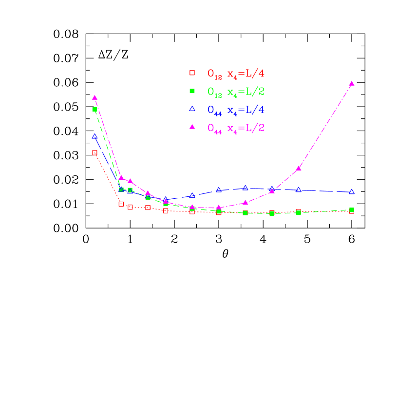
Figure 4: $\theta$-dependence of $\Delta Z/Z$. The chosen value of $\kappa$ corresponds to $m_{q}=0$. The lines only connect the points to guide the eye.

Let us start the discussion on the relative error for $Z_{{\cal O}_{12}}$. For $\theta>1$, the relative error appears to be almost constant up to $\theta=2\pi$ and independent of choosing $x_{4}/L=1/2$ or $x_{4}/L=1/4$. This means that for the operator ${\cal O}_{12}$ choosing a physical momentum (as done in our earlier work) or introducing $\theta$ would have led to the same quality of the final results.

For the operator ${\cal O}_{44}$ the situation is different, however. At $\theta=2\pi$ the relative error of $Z_{{\cal O}_{44}}$ evaluated at $x_{4}/L=1/2$ is a factor 5-6 larger than the corresponding relative error of $Z_{{\cal O}_{12}}$. For $x_{4}/L=1/4$ the situation is better, but the error is again about a factor 2 worse than for $Z_{{\cal O}_{12}}$ at least for $\theta=2\pi$. We observe a rather shallow minimum in $\theta$ starting around $\theta=1$ and ranging up to $\theta=2$ where the relative errors of the renormalization constants for both operators ${\cal O}_{12}$ and ${\cal O}_{44}$ are about the same and comparable to $\Delta Z/Z$ of $Z_{{\cal O}_{12}}(\theta=2\pi)$. The case of $Z_{{\cal O}_{44}}$ is hence an example where using $\theta$ instead of standard lattice momenta can help substantially. From Fig. 4 the value of $\theta$ to be chosen for a practical simulation can not be clearly identified. However, taken our analysis of the convergence behavior of perturbation theory, the cutoff effects as computed in 1-loop perturbation theory and the investigation of the signal to noise ratio together, we conclude that $\theta=1$ should be a reasonable choice.

3 Non-perturbative step scaling functions

Choosing the lattice regularization discussed above, is, of course, motivated by the advantage to perform numerical simulations. The aim of such simulations is to compute the lattice step scaling functions of eq. (22) non-perturbatively at non-vanishing values of the lattice spacing and to perform the –well-defined– continuum limit of eq. (23). Besides the lattice step scaling function $\Sigma_{Z_{{\cal O}}}$, we will also consider $\Sigma_{{\bar{Z}}_{{\cal O}}}$, constructed in a completely analogous way from the definition of the renormalization factors in eq. (13). In addition, we will compute the step scaling function of $f_{1}$, eq. (12),

$$\sigma_{f_{1}}(\theta)=\frac{1}{\hat{c}}\frac{\sqrt{f_{1}(sL,\theta)}}{\sqrt{f_{1}(L,\theta)}}$$ (27)

where $\hat{c}=\sqrt{f_{1}^{(0)}(sL,\theta)}/\sqrt{f_{1}^{(0)}(L,\theta)}$ is the corresponding ratio at tree-level. The lattice version $\Sigma_{f_{1}}(a/L;\theta)$ of this step scaling function is again defined in the obvious way. To complete the definition of the step scaling functions, certain choices of the values for $\theta$, $s$, $x_{4}/L$ and the quark mass $m_{q}$ have to be made. We fix these in the following to

$$x_{4}/L=1/2,\;s=2,\;\theta=1,\;m_{q}=0\;.$$ (28)

In order to justify our choice of $x_{4}/L=1/2$ we show a comparison of the step scaling function $\Sigma_{Z_{44}}$ both at $x_{4}/L=1/4$ and $x_{4}/L=1/2$ in fig. 5. Strong lattice artifacts are visible for $x_{4}/L=1/4$. Approaching the continuum limit this effect is considerably reduced, but it is clear that $\Sigma_{Z_{44}}$ is much better behaved as a function of $a/L$ when $x_{4}/L=1/2$ is chosen, which allows for a reliable (linear) continuum extrapolation.

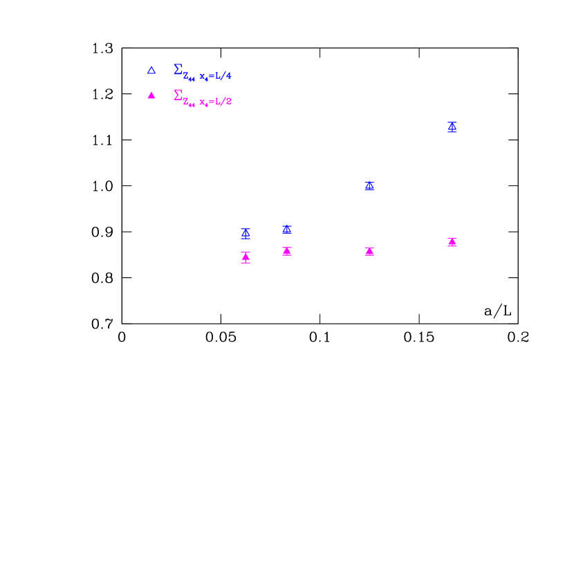
Figure 5: Lattice step scaling functions $\Sigma_{Z_{44}}(a/L)$ at $x_{4}=L/4$ and $x_{4}=L/2$ at $\bar{g}^{2}=1.8811$. The value of $\theta$ is taken from our choices in eq. (28).

With the parameter choices in eq. (28), we will in the following only give the arguments of $Z_{\cal O}$ and $\sigma_{Z_{\cal O}}$ when they differ from these values. In particular, with the choice of $s=2$ the step scaling function becomes a function of only one scale, i.e. $\sigma_{Z_{\cal O}}(\mu_{1}/\mu_{2})\rightarrow\sigma_{Z_{\cal O}}(\mu)$ and correspondingly the lattice step scaling function will only depend on the scale $\mu$ (given by a fixed value of $\bar{g}(L)$) and $a/L$.

As already discussed above, the continuum limit of $\Sigma_{Z_{\cal O}}(\bar{g}^{2}(L),a/L)$ is to be taken at a fixed value of the renormalization scale $\mu=1/L$ in order to obtain the desired continuum step scaling function $\sigma_{Z_{\cal O}}(\bar{g}^{2}(L))$. Fixing the scale is realized by fixing the renormalized coupling $\bar{g}^{2}(L)$, which in turn can be achieved by changing the value of the bare coupling as the value of the lattice spacing (and correspondingly $a/L$) is decreased. Using the SF scheme, the matching points of the bare coupling $g_{0}$ to keep $\bar{g}^{2}(L)$ fixed when the lattice spacing is sent to zero can be found in [18]. Of course, the values of $\Sigma_{Z_{\cal O}}(\bar{g}^{2}(L),a/L)$ themselves have to be computed in a numerical simulation on lattices with increasing number of points $N^{4}=(L/a)^{4}$ as $a\rightarrow 0$.

As in our previous work, we will choose two different lattice discretizations, standard Wilson fermions and non-perturbatively O(a)-improved (clover) fermions to compute the step scaling function $\Sigma_{Z_{\cal O}}(\bar{g}^{2}(L),a/L)$. Since we want to employ a massless renormalization scheme and have to stay therefore at zero quark, we take from [18] the values of $\kappa_{c}$ for clover fermions to stay in the massless limit. For the case of Wilson fermions, we determined $\kappa_{c}$ ourselves (see table 2).

$\overline{g}_{SF}^{2}$	$L/a$	$\beta\quad\quad$	$\;\;\kappa_{c}[Wilson]$	$\;\;\kappa_{c}[Clover]$
$~{}0.8873$	$6$	$~{}10.7503~{}$	$~{}0.134696(7)$	$~{}0.130591(4)$
	$8$	$~{}11.0000~{}$	$~{}0.134548(6)$	$~{}0.130439(3)$
	$12$	$~{}11.3384~{}$	$~{}0.134277(5)$	$~{}0.130251(2)$
	$16$	$~{}11.5736~{}$	$~{}0.134068(6)$	$~{}0.130125(2)$
$1.0989$	$6$	$~{}9.5030~{}$	$~{}0.136520(5)$	$~{}0.131514(5)$
	$8$	$~{}9.7500~{}$	$~{}0.136310(3)$	$~{}0.131312(3)$
	$12$	$~{}10.0577~{}$	$~{}0.135949(4)$	$~{}0.131079(3)$
	$16$	$~{}10.3419~{}$	$~{}0.135572(4)$	$~{}0.130876(2)$
$1.3293$	$6$	$~{}8.6129~{}$	$~{}0.138346(6)$	$~{}0.132380(6)$
	$8$	$~{}8.8500~{}$	$~{}0.138057(4)$	$~{}0.132140(5)$
	$12$	$~{}9.1859~{}$	$~{}0.137503(2)$	$~{}0.131814(3)$
	$16$	$~{}9.4381~{}$	$~{}0.137061(4)$	$~{}0.131589(2)$
$1.5533$	$6$	$~{}7.9993~{}$	$~{}0.140003(11)$	$~{}0.133118(7)$
	$8$	$~{}8.2500~{}$	$~{}0.139588(8)$	$~{}0.132821(5)$
	$12$	$~{}8.5985~{}$	$~{}0.138847(6)$	$~{}0.132427(3)$
	$16$	$~{}8.8323~{}$	$~{}0.138339(7)$	$~{}0.132169(3)$
$1.8811$	$6$	$~{}7.4082~{}$	$~{}0.142145(11)$	$~{}0.133961(8)$
	$8$	$~{}7.6547~{}$	$~{}0.141572(9)$	$~{}0.133632(6)$
	$12$	$~{}7.9993~{}$	$~{}0.140597(6)$	$~{}0.133159(4)$
	$16$	$~{}8.2415~{}$	$~{}0.139900(6)$	$~{}0.132847(3)$
$2.1000$	$6$	$~{}7.1214~{}$	$~{}0.143416(11)$	$~{}0.134423(9)$
	$8$	$~{}7.3632~{}$	$~{}0.142749(9)$	$~{}0.134088(6)$
	$12$	$~{}7.6985~{}$	$~{}0.141657(6)$	$~{}0.133599(4)$
	$16$	$~{}7.9560~{}$	$~{}0.140817(7)$	$~{}0.133229(3)$
$2.4484$	$6$	$~{}6.7807~{}$	$~{}0.145286(11)$	$~{}0.134994(11)$
	$8$	$~{}7.0197~{}$	$~{}0.144454(7)$	$~{}0.134639(7)$
	$12$	$~{}7.3551~{}$	$~{}0.143113(6)$	$~{}0.134141(5)$
	$16$	$~{}7.6101~{}$	$~{}0.142107(6)$	$~{}0.133729(4)$
$2.7700$	$6$	$~{}6.5512~{}$	$~{}0.146825(11)$	$~{}0.135327(12)$
	$8$	$~{}6.7860~{}$	$~{}0.145859(7)$	$~{}0.135056(8)$
	$12$	$~{}7.1190~{}$	$~{}0.144299(8)$	$~{}0.134513(5)$
	$16$	$~{}7.3686~{}$	$~{}0.143113(?)$	$~{}0.134114(3)$
$3.4800$	$6$	$~{}6.2204~{}$	$~{}0.149685(15)$	$~{}0.135470(15)$
	$8$	$~{}6.4527~{}$	$~{}0.148391(9)$	$~{}0.135543(9)$
	$12$	$~{}6.7750~{}$	$~{}0.146408(7)$	$~{}0.135121(5)$
	$16$	$~{}7.0203~{}$	$~{}0.145025(8)$	$~{}0.134707(4)$

Table 2: Simulation Parameters

Simulations have been performed on APEmille machines using even–sized lattices ranging from $6^{4}$ to $32^{4}$. We recall that for both actions we used the unimproved operator: as a consequence, the results at finite values of the lattice spacing are affected by lattice artefacts of O$(a)$, whose precise form depends upon the choice of the lattice action.

For the inversion of the Dirac operator we used the implementation [19] of the SSOR-preconditioned BiCGStab inverter [20]. The gauge fields were generated with a hybrid of Cabibbo–Marinari heat–bath and over–relaxation updates: we decided to keep the number of over–relaxation steps between a single heat-bath one proportional to $L/a$ (in practice $N_{\rm or}=\frac{1}{2}L/a$). A full update sweep is defined as one heat–bath step followed by $N_{\rm or}$ steps: in order to statistically decorrelate the gauge configurations used to take measurements of our observables, we allowed for a number of full sweeps between measurements ranging from 20 (lattices up to $L/a=16$) to 70 ($L/a=32$).

As usual in this kind of finite–size–step simulations, the signal over noise ratio deteriorates for larger values of $\bar{g}^{2}$, in the fully non–perturbative regime. In order to maintain constant, up to a certain degree, the relative statistical errors on our observables, we are obliged to increase the statistics. For example, in the clover case and on $L/a=32$ lattices, the number of measurements has to grow from around 300 at the smallest values of $\bar{g}^{2}$ up to order 700 at the largest value of the renormalized coupling. Accordingly, for lattices with a smaller number of space–time points, the number of measurements grows from 500 to 2000. The pattern for the Wilson case is similar, albeit with an overall smaller statistical sample.

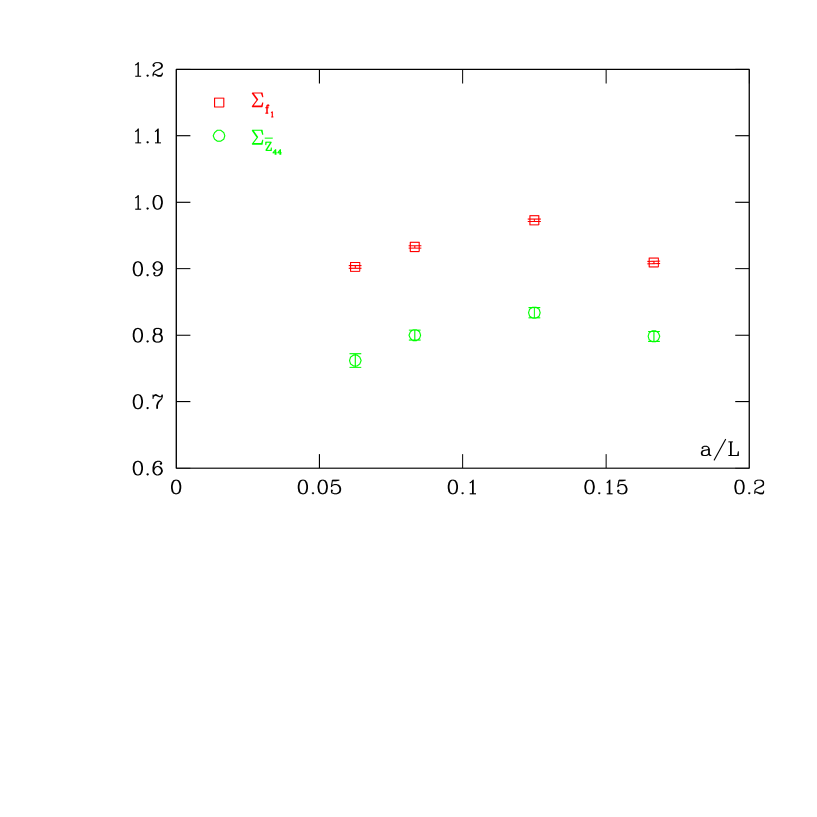
Figure 6: Lattice step scaling functions $\Sigma_{f_{1}}(\bar{g}^{2}(L),a/L)$ and $\Sigma_{\bar{Z}_{44}}(\bar{g}^{2}(L),a/L)$ at $\bar{g}^{2}=1.8811$. The values of $\theta$ and $x_{4}/L$ are taken from our choices in eq. (28).

In Fig. 6 we show separately the lattice step scaling functions $\Sigma_{\bar{Z}_{44}}(\bar{g}^{2}(L),a/L)$ and $\Sigma_{f_{1}}(\bar{g}^{2}(L),a/L)$ at four values of $a/L$ for $\bar{g}^{2}$ fixed. Both step scaling functions show rather large lattice artefacts. For $\Sigma_{f_{1}}$ this behavior is in sharp contrast to the case of choosing $\theta=0$, where the $a/L$ dependence of $\Sigma_{f_{1}}$ is basically flat, at least in the O(a)-improved theory [3, 4]. This flat behavior led us, in our earlier work, to the conclusion to perform the continuum limit of $\Sigma_{\bar{Z}_{12}}$ and $\Sigma_{f_{1}}$ separately and to compute the desired continuum step scaling function $\sigma_{Z_{12}}=\sigma_{\bar{Z}_{12}}/\sigma_{f_{1}}$ after the continuum limit of $\Sigma_{\bar{Z}_{12}}$ and $\Sigma_{f_{1}}$ had been performed.

The example of the step scaling functions, shown in Fig. 6, indicates that for $\theta$ non-vanishing the strategy might be different. Indeed, we found in the analysis of our data –for $\theta=1$– that in the ratios

$$\Sigma_{\bar{Z}_{44}}(\bar{g}^{2}(L),a/L)/\Sigma_{f_{1}}(\bar{g}^{2}(L),a/L)$$ (29)

and

$$\Sigma_{\bar{Z}_{12}}(\bar{g}^{2}(L),a/L)/\Sigma_{f_{1}}(\bar{g}^{2}(L),a/L)$$ (30)

the lattice artefacts essentially cancel. This cancellation happens for clover as well as for Wilson fermions. We decided therefore that for our choice of $\theta=1$ to first compute

$$\Sigma_{Z}(\bar{g}^{2}(L),a/L)=\Sigma_{\bar{Z}}(\bar{g}^{2}(L),a/L)/\Sigma_{f_{1}}(\bar{g}^{2}(L),a/L)$$ (31)

at a given value of $a/L$ and then perform the continuum limit.

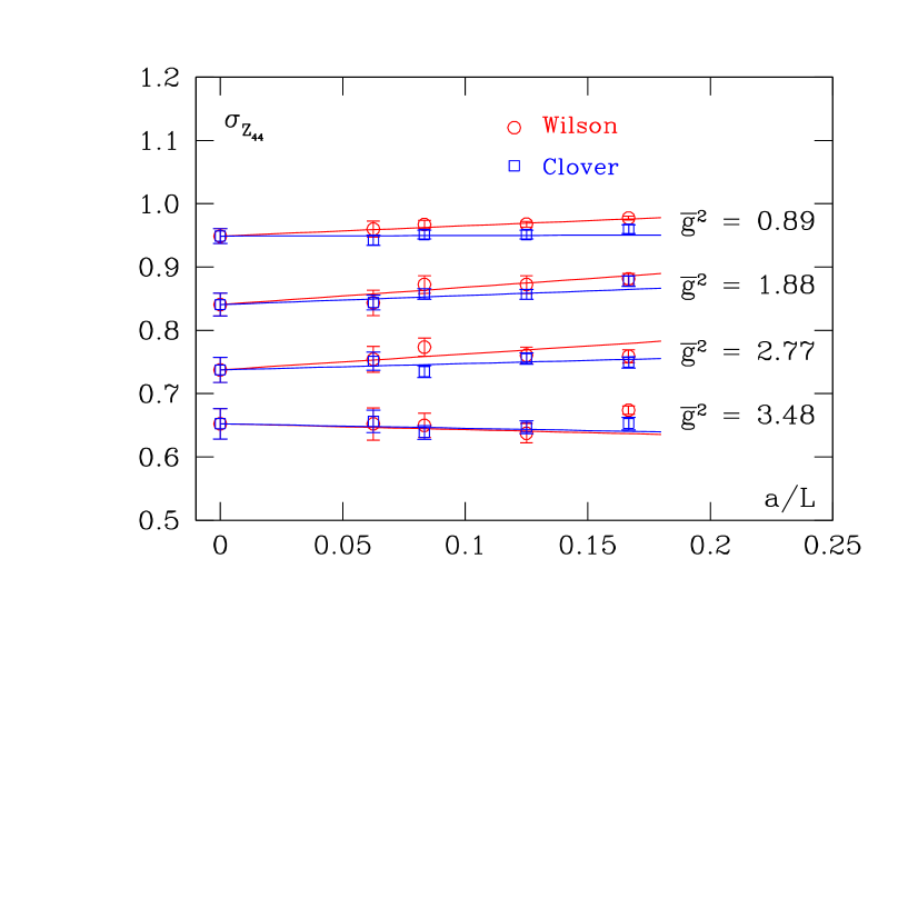
Figure 7: Examples of the continuum limit of step scaling functions for both Wilson and clover fermions. The (constrained) fit performed is linear, taking the 3 data points with smallest values of $a/L$. We also indicate the values of the running coupling that correspond to these step scaling functions.

In Fig. 7 we show examples of the continuum extrapolations of $\Sigma_{{\cal O}_{44}}$ for both discretization, Wilson and clover fermions. It can be observed that in both cases the continuum extrapolation is linear in the lattice spacing when the data points with the three smallest values of $a/L$ are taken. In the plot we show already a constraint fit, demanding that both set of lattice results extrapolate to the same value of the continuum step scaling function. We obtain a very similar plot for $\Sigma_{{\cal O}_{12}}$. The numerical results of the continuum extrapolation as well as for the four lattice spacings are summarized in table 3 for the ${\cal O}_{12}$ and in table 4 for the ${\cal O}_{44}$ operator.

One subtlety, we want to mention, is that even in the continuum limit at fixed scale, the step scaling functions of ${\cal O}_{44}$ and ${\cal O}_{12}$ do not assume the same value. The reason is that both operators belong to two different representations and in the here adopted finite volume renormalization scheme they are therefore also part of the precise definition of the scheme. It is hence not possible, to constrain the fits even more by demanding that $\Sigma_{{\cal O}_{44}}$ and $\Sigma_{{\cal O}_{12}}$ converge to the same value of the continuum step scaling function.

4 Running and invariant step scaling function

At this stage, we can leave the lattice and discuss continuum quantities only. The only reminder that we have performed a lattice calculation is that we will stay in the somewhat unusual, finite volume SF renormalization scheme. The simulations described in the previous section provide us with the continuum step scaling functions $\sigma_{Z_{44}}$ and $\sigma_{Z_{12}}$ at a number of values for the running coupling $0.8<\bar{g}^{2}<3.5$, corresponding to a wide range of scales, $500\;\mathrm{MeV}<\mu<100\;\mathrm{GeV}$.

Figure 8: Continuum step scaling function $\sigma_{Z_{44}}$. The solid line represents the parameterization eq. (32), the dotted line represents the the 1-loop, the dashed line the 2-loop predictions from perturbation theory.

In Fig. 8 we show the continuum step scaling function $\sigma_{Z_{44}}$ as a function of the running coupling (and hence the scale). The dotted curve is the 1-loop perturbative analysis for the step scaling function, whereas the dashed curve is a 2-loop result, taking the 2-loop anomalous dimension in the SF scheme from its relation to the 2-loop anomalous dimension in the $\overline{\mathrm{MS}}$-scheme discussed in section 2.1. The solid line is a fit to the data according to the formula

$$\sigma_{Z_{44}}=1-\gamma_{0}\ln(2)g_{0}^{2}+c_{1}g_{0}^{4}+c_{2}g_{0}^{6}\;.$$ (32)

In eq. (32) we have taken the known 1-loop ($\gamma_{0}$) and fitted only the coefficients $c_{1},c_{2}$ which we find to be $c_{1}=-0.0334(50),\;c_{2}=0.0041(18)$. It can be seen from the figure that 1-loop perturbation theory is not a good description of the data at all. Even 2-loop perturbation theory represents the data only up to $\bar{g}^{2}=2$, or so.

Figure 9: Continuum step scaling function $\sigma_{Z_{12}}$. The solid line represents the parameterization eq. (32), the dotted line represents the the 1-loop, the dashed line the 2-loop predictions from perturbation theory. We also show the values of $\sigma_{Z_{12}}$ for $\theta=2\pi$ (open symbols) corresponding to a minimal physical momentum.

Fig. 9 is the same as fig. 8 for the operator ${\cal O}_{12}$. In this case we find the coefficients $c_{1}=-0.0343(41),\;c_{2}=0.0049(14)$ for the parameterization of eq. (32). In addition, we show the values of the step scaling function $\sigma_{Z_{12}}^{p}$ as obtained in our earlier work, i.e. using $\theta=0$ and a momentum $p=2\pi/L$ (open symbols). Clearly, the scale dependence of $\sigma_{Z_{12}}(\theta=1)$ is much stronger than for $\sigma_{Z_{12}}^{p}$.

The final result of this paper is the (ultra-violet) invariant step scaling function for the operators ${\cal O}_{44}$ and ${\cal O}_{12}$ as they are needed to describe the running of the physical matrix element in other schemes than the SF one. We adopt here the definition of the invariant step scaling function as given in [5]:

$$\EuFrak{S}_{\rm INV}^{\rm UV,SF}(\mu_{0})=\sigma(\mu/\mu_{0},\bar{g}^{2}(L_{0}))\cdot(\bar{g}^{2}(L))^{-\gamma_{0}/2b_{0}}\exp\left\{-\int_{0}^{\bar{g}(\mu)}dg\left[\frac{\gamma(g)}{\beta(g)}-\frac{\gamma_{0}}{b_{0}g}\right]\right\}\;.$$ (33)

The $\beta$- and $\gamma$-functions in eq. (33) will be taken to a given order in perturbation theory in the SF scheme. A scheme dependence is still manifest in $\EuFrak{S}_{\rm INV}$ through the appearance of the infra-red scale ($\mu_{0}=L_{0}^{-1}$). We thus add a superscript to indicate that the invariant step scaling function is computed within the Schrödinger functional scheme.

For large enough scales in the ultra-violet, it is expected that the running of the step scaling functions, as computed non-perturbatively above, will match the perturbative running and hence that $\EuFrak{S}_{\rm INV}$ will become independent from the scale. In order to test at which scales $\EuFrak{S}_{\rm INV}$ becomes constant, we have to evolve the step scaling functions starting from our most non-perturbative scale $\mu_{0}=(1/2L_{\rm{max}})$, implicitly given by $\bar{g}^{2}(2L_{\rm{max}})=3.48$. One finds [21] $2L_{\rm{max}}=(1.476r_{0})$, where $r_{0}\approx 0.5\mathrm{fm}$. The step scaling functions $\sigma_{Z_{\cal O}}$ are only computed at certain values of $\bar{g}^{2}(L)$. Subsequent values of $\bar{g}^{2}(L)$ do, however, not correspond to a scale change by a factor of two as needed. In order to find the precise evolution by steps of two an interpolation in $\bar{g}^{2}(L)$ has to be performed using the parameterization of eq. (32). The corresponding values of the step scaling function can be found in table 5.

The error of the so obtained values of $\sigma_{Z_{\cal O}}$ is evaluated by a standard error propagation taking the correlation of the fit parameters into account through the covariance matrix (cov), i.e.

$$(\Delta\sigma_{Z_{\cal O}})=\sqrt{\frac{\partial\sigma_{Z_{\cal O}}}{\partial c_{1}}^{2}(\Delta c_{1})^{2}+\frac{\partial\sigma_{Z_{\cal O}}}{\partial c_{2}}^{2}(\Delta c_{2})^{2}+2\frac{\partial\sigma_{Z_{\cal O}}}{\partial c_{1}}\cdot\frac{\partial\sigma_{Z_{\cal O}}}{\partial c_{2}}\cdot\mathrm{cov}_{12}}+\frac{\partial\sigma_{Z_{\cal O}}}{\partial\bar{g}^{2}}\Delta\bar{g}^{2}\;.$$ (34)

As an aside we mention that we also have seen that the errors coming from the uncertainty in $\bar{g}^{2}(L)$ are not negligible, and they are included in the values given in table 5. In evaluating $\EuFrak{S}_{\rm INV}$ in eq. (33) we have taken the 3-loop $\beta$-function and the 2-loop $\gamma$-function.

In Fig. 10 we show $\EuFrak{S}_{\rm INV}$ as a function of $\mu/\Lambda_{\mathrm{SF}}^{(0)}$ with $\Lambda_{\mathrm{SF}}^{(0)}\approx 120\;\mathrm{MeV}$ being the $\Lambda$-parameter in the quenched approximation in the SF scheme. For the operator ${\cal O}_{44}$ (full symbols) the invariant step scaling function is constant for, say, $\mu/\Lambda_{\mathrm{SF}}^{(0)}>50$ indicating that contact with perturbation theory can safely be made. In the same figure we also show the value of the invariant step scaling function for ${\cal O}_{12}$ which shows a very similar behavior. The fact that both invariant step scaling functions assume different values indicates again that the two different operators define two different renormalization schemes, at least in a finite volume scheme like the SF. The difference will only disappear in the physical renormalization group invariant matrix element.

In order to obtain finally the values of the invariant step scaling functions, we have taken the values at the corresponding largest scale:

$$\EuFrak{S}_{\rm INV,{\cal O}_{12}}^{UV,SF}(\mu_{0})=0.242(8),\;\EuFrak{S}_{\rm INV,{\cal O}_{44}}^{UV,SF}(\mu_{0})=0.221(9)\;.$$ (35)

As a comparison we quote the value of $\EuFrak{S}_{\rm INV,{\cal O}_{12}}^{UV,SF}(\mu_{0})=1.11(4)$ as obtained at $\theta=0$ and $p=2\pi/L$ in our previous work.

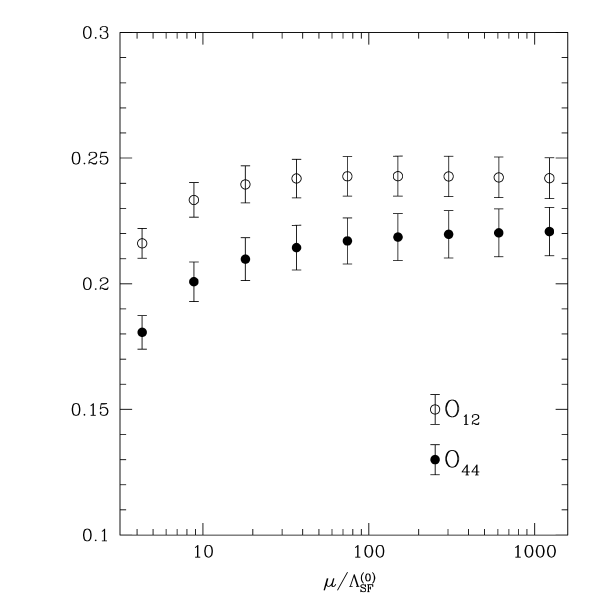
Figure 10: The RG invariant step scaling function for the operator ${\cal O}_{44}$ (full symbols) and the operator ${\cal O}_{12}$ (open symbols).

5 Conclusion

In this paper we have demonstrated how the generalized boundary conditions advocated in ref. [1] can to utilized to define continuous external momenta as often needed in the lattice simulations when operators with derivatives are considered. We investigated the particular example of a scale dependent renormalization constant for renormalizing twist-2 non-singlet quark operators corresponding to moments of parton distribution functions.

Although we demonstrated the usefulness for such momentum definitions for a renormalization constant, or more specific its step scaling function, it is clear that in principle the same method also applies to matrix elements themselves, as long as no real physical momentum transfer is involved. The feasibility of this approach has to be tested, however, in a real numerical benchmark simulation.

For the particular example at hand, we could determine the renormalization constant for a certain lattice representation of a continuum operator that determines the average (quark) momentum in a hadron. Such a calculation would have been very difficult by using standard, quantized lattice momenta as usually taken. As a result, we could determine the RG invariant step scaling function for two different lattice representations of the same continuum operator. In this way, we could eliminate a small systematic uncertainty that plagued our earlier work.

The idea of the present work was to show the practicability and usefulness of the generalized momentum definition on a practical example. The values of the RG invariant step scaling we have computed are essential ingredients for the RG invariant matrix elements which allow a comparison with experimental data or global fits. Results for these physical matrix elements, in which we are finally interested in, will be reported in a forthcoming publication.

Acknowledgments

We thank S. Capitani, R. Sommer and S. Sint for many useful discussions. The computer center at NIC/DESY Zeuthen provided the necessary technical help and the computer resources. This work was supported by the EU IHP Network on Hadron Phenomenology from Lattice QCD and by the DFG Sonderforschungsbereich/Transregio SFB/TR9-03.

$\bar{g}_{SF}^{2}$	$a/L$	$\Sigma_{Z_{12}}[Wilson]$	$\Sigma_{Z_{12}}[Clover]$	$~{}~{}~{}~{}~{}~{}\sigma_{Z_{12}}$	$\chi^{2}/dof$
	1/6	0.9937(25)	0.9682(60)
0.8873	1/8	0.9787(34)	0.9616(59)	0.9475(96)	0.32
	1/12	0.9640(55)	0.9571(58)
	1/16	0.9689(94)	0.9555(71)
	1/6	0.9899(39)	0.9540(58)
1.0989	1/8	0.9727(55)	0.9591(62)	0.9211(105)	0.23
	1/12	0.9608(67)	0.9446(61)
	1/16	0.9480(91)	0.9368(74)
	1/6	0.9771(42)	0.9360(69)
1.3293	1/8	0.9680(61)	0.9365(67)	0.8905(120)	0.79
	1/12	0.9339(81)	0.9305(66)
	1/16	0.9230(117)	0.9157(81)
	1/6	0.9716(48)	0.9153(64)
1.5553	1/8	0.9545(77)	0.9102(67)	0.8896(129)	0.26
	1/12	0.9287(92)	0.9068(63)
	1/16	0.9133(132)	0.9031(86)
	1/6	0.9607(68)	0.8984(75)
1.8811	1/8	0.9259(104)	0.8778(70)	0.8522(144)	1.07
	1/12	0.9060(103)	0.8781(72)
	1/16	0.8682(153)	0.8640(93)
	1/6	0.9627(68)	0.8700(71)
2.1000	1/8	0.9107(74)	0.8592(70)	0.8419(131)	1.01
	1/12	0.8981(101)	0.8558(72)
	1/16	0.8827(102)	0.8368(99)
	1/6	0.9467(67)	0.8217(75)
2.4484	1/8	0.8811(85)	0.8223(77)	0.8064(133)	0.78
	1/12	0.8589(136)	0.8053(77)
	1/16	0.8519(85)	0.8116(107)
	1/6	0.9309(75)	0.7864(75)
2.7700	1/8	0.8759(94)	0.7838(78)	0.7395(157)	0.77
	1/12	0.8385(102)	0.7593(75)
	1/16	0.8225(152)	0.7583(118)
	1/6	0.9063(50)	0.7176(83)
3.4800	1/8	0.8203(110)	0.6899(86)	0.6793(187)	0.56
	1/12	0.7846(144)	0.6761(89)
	1/16	0.7604(191)	0.6851(136)

Table 3: Results for the lattice step scaling function $\Sigma_{Z_{12}}$ and the combined continuum extrapolation $\sigma_{Z_{12}}$ of Wilson and Clover data with the three smallest lattice spacings.

$\bar{g}_{SF}^{2}$	$a/L$	$\Sigma_{Z_{44}}[Wilson]$	$\Sigma_{Z_{44}}[Clover]$	$~{}~{}~{}~{}~{}~{}\sigma_{Z_{44}}$	$\chi^{2}/dof$
	1/6	0.9776(30)	0.9596(68)
0.8873	1/8	0.9677(44)	0.9513(68)	0.9489(115)	0.49
	1/12	0.9671(65)	0.9514(68)
	1/16	0.9601(125)	0.9425(81)
	1/6	0.9577(49)	0.9375(66)
1.0989	1/8	0.9560(69)	0.9421(71)	0.9234(128)	0.50
	1/12	0.9505(85)	0.9420(71)
	1/16	0.9330(123)	0.9290(86)
	1/6	0.9402(54)	0.9184(77)
1.3293	1/8	0.9416(81)	0.9275(77)	0.8943(145)	1.40
	1/12	0.9250(104)	0.9322(78)
	1/16	0.9118(153)	0.9037(93)
	1/6	0.9062(63)	0.8908(71)
1.5553	1/8	0.9163(100)	0.8977(75)	0.8900(154)	1.60
	1/12	0.9140(117)	0.9084(74)
	1/16	0.8834(163)	0.8873(103)
	1/6	0.8813(88)	0.8777(84)
1.8811	1/8	0.8723(140)	0.8569(80)	0.8407(178)	0.54
	1/12	0.8723(139)	0.8577(84)
	1/16	0.8434(199)	0.8439(117)
	1/6	0.8698(88)	0.8354(80)
2.1000	1/8	0.8467(97)	0.8399(82)	0.8373(157)	1.75
	1/12	0.8545(133)	0.8425(84)
	1/16	0.8590(129)	0.8181(112)
	1/6	0.8197(88)	0.8016(89)
2.4484	1/8	0.7935(119)	0.7885(91)	0.7944(169)	0.55
	1/12	0.7942(186)	0.7921(94)
	1/16	0.7823(115)	0.8036(127)
	1/6	0.7589(103)	0.7494(88)
2.7700	1/8	0.7606(129)	0.7556(90)	0.7376(197)	1.22
	1/12	0.7736(143)	0.7347(92)
	1/16	0.7542(203)	0.7512(143)
	1/6	0.6739(66)	0.6528(99)
3.4800	1/8	0.6376(153)	0.6469(104)	0.6525(241)	0.34
	1/12	0.6500(193)	0.6385(110)
	1/16	0.6522(256)	0.6563(178)

Table 4: Results for the lattice step scaling function $\Sigma_{Z_{44}}$ and the combined continuum extrapolation $\sigma_{Z_{44}}$ of Wilson and Clover data with the three smallest lattice spacings.

$\bar{g}_{SF}^{2}$	$\sigma_{Z_{12}}$	$\sigma_{Z_{44}}$
3.480	0.6826(169)	0.6579(216)
2.454(18)	0.7893(83)	0.7822(100)
1.918(18)	0.8486(76)	0.8458(90)
1.584(18)	0.8840(67)	0.8828(79)
1.353(18)	0.9071(58)	0.9066(68)
1.184(17)	0.9231(50)	0.9229(58)
1.053(15)	0.9348(42)	0.9348(49)
0.950(14)	0.9436(37)	0.9437(42)
0.865(13)	0.9505(32)	0.9506(37)

Table 5: Interpolated values of the step scaling function $\sigma_{Z_{12}}$ and $\sigma_{Z_{44}}$ for the scale change by a factor two.

Appendix A

In this appendix we recall some basic properties of the renormalization group functions. For small couplings the $\beta$-function and the anomalous dimension ($\gamma$-function), defined by

 

$${\beta(g)}$$

  (36)

have asymptotic expansions of the form

 

$${\beta(g)}$$

  (37)

One finds that $b_{0}$, $b_{1}$ and $\gamma_{0}$ are the same in all the schemes (these are the “universal” coefficients), while all other coefficients are scheme dependent. The universal coefficients are given by (with $C_{F}=(N_{c}^{2}-1)/2N_{c}$ and $N_{c}$ the number of colors)

$$b_{0} = \bigl{\{}\frac{11}{3}N_{c}-\frac{2}{3}N_{\rm f}\bigr{\}}(4\pi)^{-2},$$ (38)

$$\gamma_{0} = \frac{16}{3}C_{F}(4\pi)^{-2},$$ (39)

$$b_{1} = \bigl{\{}\frac{34}{3}N_{c}^{2}-(\frac{13}{3}N_{c}-N_{c}^{-1})N_{\rm f}\bigr{\}}(4\pi)^{-4}.$$ (40)

Any two mass independent renormalization schemes can be related by a scale change and a finite parameter renormalization of the form

$$\mu^{\prime} = c\mu,\qquad c>0,$$ (41)

$$\bar{g}^{\prime} = \bar{g}\sqrt{{\cal X}_{\rm g}(\bar{g})},$$ (42)

$$Z^{\prime} = Z[\Delta Z_{{\cal O}}(\bar{g})],$$ (43)

where $c$ is just a change of scale between the 2 schemes and one could obviously choose also $c=1$. ${\cal X}_{\rm g}$ and $\Delta Z_{{\cal O}}$ are expanded according to

$${\cal X}_{\rm g}(\bar{g})\buildrel{\bar{g}}\rightarrow 0\over{\sim}1+\sum_{k=1}^{\infty}{\cal X}_{\rm g}^{(k)}\bar{g}^{2k}.$$ (44)

$$\Delta Z_{{\cal O}}(\bar{g})\buildrel{\bar{g}}\rightarrow 0\over{\sim}1+\sum_{k=1}^{\infty}\Delta Z_{{\cal O}}^{(k)}\bar{g}^{2k}.$$ (45)

The invariance of a physical observable under such a change of parameters, gives a relation between the renormalization group functions, $\beta$ and $\gamma$, in the 2 schemes. In particular we have

$$\gamma_{1}=\gamma_{1}^{\overline{\mathrm{MS}}}+2b_{0}\Delta Z_{{\cal O}}^{(1)}-\gamma_{0}{\cal X}_{\rm g}^{(1)}.$$ (46)

From ref. [22] we have

$${\cal X}^{(1)}_{\rm g}=-{1\over 4\pi}(c_{1,0}+c_{1,1}N_{\rm f}),$$ (47)

with

$$c_{1,0}=1.25563(4),\qquad c_{1,1}=0.039863(2).$$ (48)

From the perturbative results in [16] (section 2.1) it is possible to obtain $\Delta Z_{{\cal O}}^{(1)}$.

References

-
[1]
K. Jansen, C. Liu, M. Lüscher, H. Simma, S. Sint, R. Sommer,
P. Weisz and U. Wolff, Phys. Lett. B372 (1996) 275;
M. Lüscher, S. Sint, R. Sommer and P. Weisz, Nucl. Phys. B478 (1996) 365. - [2] A. Bucarelli, F. Palombi, R. Petronzio and A. Shindler, Nucl. Phys. B552 (1999) 379.
- [3] M. Guagnelli, K. Jansen and R. Petronzio, Nucl. Phys. B542 (1999) 395.
- [4] M. Guagnelli, K. Jansen and R. Petronzio, Phys. Lett. B457 (1999) 153.
- [5] M. Guagnelli, K. Jansen and R. Petronzio, Phys. Lett. B459 (1999) 594.
- [6] M. Guagnelli, K. Jansen, R. Petronzio, Phys.Lett. B493 (2000) 77.
-
[7]
M. Lüscher, R. Narayanan, P. Weisz and U. Wolff, Nucl. Phys. B384 (1992) 168;
S.Sint, Nucl. Phys. B421 (1994) 135. - [8] talk presented by K. Jansen at the XXXth International Conference on High Energy Physics (ICHEP 2000), July 27-August 2, 2000, hep-lat/0010038.
- [9] M. Guagnelli, K. Jansen, F. Palombi, R. Petronzio, A. Shindler and I. Wetzorke, plenary talk given by A. Shindler Electron-Nucleus Scattering VII, June 24-28, 2002, Elba, to be published in Eur. J.A.
- [10] M. Guagnelli, K. Jansen, F. Palombi, R. Petronzio, A. Shindler and I. Wetzorke, to be published by World Scientific, proceedings of conference GDH 2002, July 3-6 2002, Genova.
-
[11]
M. Baake, B. Gemünden and R.Oedingen, J. Math. Phys. 23 (1982) 944;
J.E.Mandula, G.Zweig and J.Govaerts, Nucl. Phys. B228 (1983) 91. - [12] S. Sint, Nucl. Phys. B451 (1995) 416.
- [13] M. Lüscher and P. Weisz, Nucl. Phys. B479 (1996) 429.
- [14] F. Palombi, R. Petronzio and A. Shindler, Nucl. Phys. B637 (2002) 243.
- [15] S. Sint, P. Weisz, Nucl. Phys. B545 (1999) 529.
- [16] S. Capitani, Lattice perturbation theory, hep-lat/0211036.
- [17] B. Sheikholeslami, R. Wohlert, Nucl. Phys. B259 (1985) 572.
-
[18]
M. Lüscher, R. Sommer, P. Weisz and U. Wolff,
Nucl. Phys. B389 (1993) 247; Nucl. Phys. B413 (1994) 481;
S.Capitani et al., Nucl. Phys. B (Proc. Suppl.) 63 (1998) 153. - [19] ALPHA, M. Guagnelli and J. Heitger, Comput. Phys. Commun. 130 (2000) 12 [hep-lat/9910024]
- [20] S. Fischer et al., Comput. Phys. Commun. 98 (1996) 20 [hep-lat/9602019]
- [21] S. Necco, R. Sommer Nucl. Phys. B622 (2002) 328
- [22] S. Sint, R. Sommer, Nucl. Phys. B465 (1996) 71.