Renormalization of Anisotropy and Glueball Masses on Tadpole Improved Lattice Gauge Action

Abstract

The Numerical calculations for tadpole-improved $U(1)$ lattice gauge theory in three-dimensions on anisotropic lattices have been performed using standard path integral Monte Carlo techniques. Using average plaquette tadpole renormalization scheme, simulations were done with temporal lattice spacings much smaller than the spatial ones and results were obtained for the string tension, the renormalized anisotropy and scalar glueball masses. We find, by comparing the ‘regular’ and ‘sideways’ potentials, that tadpole improvement results in very little renormalization of the bare anisotropy and reduces the discretization errors in the static quark potential and in the glueball masses.

I Introduction

Compact $U(1)$ gauge theory in (2+1) dimensions is one of the simplest models with dynamical gauge degrees of freedom and possesses some important similarities with QCD ham94 . The model has two essential features in common with QCD, confinement pol77 ; pol78 and chiral symmetry breaking fie90 . The theory is interesting in its own right, for it has analytically been shown to confine electrically charged particles even in the weak-coupling regime (at zero temperature)pol77 ; pol78 ; ban77 ; banks78 ; dre79 ; gof82 . The confinement is understood as a result of the dynamics of the monopoles which emerge due to the compactness of the gauge field. The string tension as a function of the coupling behaves in a similar fashion to that of the 4-dimensional $SU(N)$ lattice gauge theory. This model also allows us to work with large lattices with reasonable statistics. Other common features of compact $U(1)_{(2+1)}$ and QCD are the existence of a mass gap and of a confinement-deconfinement phase transition at some non-zero temperature. Thus, being reasonably simple and theoretically well understood in the weak-coupling limit, the $U(1)$ model provides a good testing ground for the development of new methods and new algorithmic approaches. In a recent paper loan02 we have obtained the first clear picture of the static quark potential, showing very clear evidence of the linear confining behaviour at large distances. The evidence of the the scaling behaviour of the string tension and the mass gap has also been observed in this model.

In the present paper we want to extend the analysis of Ref. loan02 in various respects. Since the measured ratio of spatial to temporal lattice spacings is not the same as the input parameter in the action, it becomes important to determine the true or renormalized anisotropy $\xi_{phys.}$ as a function of the bare anisotropy $\xi_{0}$. An important advantage of using anisotropic lattices has been the need to measure the renormalization of anisotropy in the simulation. The existing theoretical snipp97 ; garcia97 and numerical studies klas98 with Wilson action for $SU(3)$ lattice gauge theory have shown that at finite coupling $g$, the renormalized anisotropy $\xi_{phys.}$ differs appreciably form bare anisotropy $\xi_{0}$. However, it has recently been shown that the use of improved actions, supplemented by tadpole improvement, besides providing a better discretization scheme for QCD, offer the advantage of a significant reduction of renormalization of $\xi_{0}$ to a few percent morn97 ; mor96 . The anisotropy parameter $\eta$ (ratio of the renormalized and bare anisotropy) and anisotropic coefficients have been calculated to one-loop order for improved actions in various recent studies garcia97 ; sakai00 ; eng00 ; alford01 ; drummond02 . These calculations have provided very reliable results and the observed behaviour is confirmed non-perturbatively by large scale simulations on fine lattices morn97 ; shakes98 ; alford98 . We investigate the influence of tadpole improvement on isotropic and anisotropic lattices for the $U(1)$ model in (2+1) dimensions in reducing the renormalization of the bare anisotropy at weak and strong couplings. We also apply tadpole improved $U(1)$ lattice gauge theory to calculations of the static quark potential, the string tension and the scalar glueball masses and compare the results with simulations of the Wilson action.

The rest of this paper is organized as follows. After outlining the tadpole improved $U(1)$ gauge model in (2+1) dimensions in Sect. II, we describe the method for determination of the renormalized anisotropy in Sect. III. We present results from our simulations on anisotropic lattices using both standard and tadpole improved Wilson gauge action in Sect. IV. We compare bare and renormalized anisotropies, static quark potential and scalar glueball masses from these actions. We conclude in Sect. V with a summary and outlook on future work.

II Compact $U(1)$ model in (2+1) dimensions

The tadpole-improved $U(1)$ gauge action on an anisotropic lattice can be written in the following form klas98 :

$$S=\beta\left[\sum_{r,i>j}\frac{\xi_{0}}{u_{s}^{4}}(1-P_{ij}(r))+\sum_{r,i}\frac{1}{\xi_{0}u_{s}^{2}u_{t}^{2}}(1-P_{it}(r))\right]$$ (1)

where $P_{\mu\nu}$ is the plaquette operator, $\xi_{0}=\Delta\tau=a_{t}/a_{s}$ is the bare anisotropy at the classical level and $u_{s}$ and $u_{t}$ are the mean fields for the tadpole improvement. The notation used in Eq.(1) differ slightly from that used in Refs. garcia97 ; drummond02 , where the spatial and temporal mean-field improvement factors, $u_{s}$ and $u_{t}$ were absorbed into definition of $\beta$ and $\xi_{0}$. This, however, follows the notation introduced in Ref. morn97 .

On the anisotropic lattice, the mean fields are determined using the measured values of the average plaquettes mor97 . We first compute $u_{s}$ from spatial plaquettes, $u_{s}^{4}=\langle P_{ij}\rangle$, and then we compute $u_{t}$ from temporal plaquettes, $u_{t}^{2}u_{s}^{2}=\langle P_{it}\rangle$. Another way to determine the mean fields is to use the mean links in Landau gauge lep98

$$u_{t}=\langle\mbox{ReTr}U_{t}\rangle,\hskip 28.45274ptu_{s}=\langle\mbox{ReTr}U_{i}\rangle$$ (2)

where the lattice version of the gauge condition is obtained by maximizing the quantity,

$$\sum_{r,\mu}\frac{1}{u_{\mu}a_{\mu}^{2}}\mbox{Tr}U_{\mu}(r)$$ (3)

Since the temporal lattice spacing in our simulations is very small, we adopt the following convention mor97 ; mor96 ; morn97 for the mean fields in tadpole improvement

$$u_{t}\equiv 1,\hskip 28.45274ptu_{s}=\langle P_{ij}\rangle^{1/4}.$$ (4)

This prescription eliminates the need for gauge fixing and the results yield values for $u_{s}$ which differ from those using Landau gauge by only a few percent.

III Renormalization of Anisotropy

Following the procedure of Klassen klas98 and Shakespeare and Trottier shakes98 , we measure the static quark potential extracted from Wilson loops in the spatial and temporal directions. Accordingly on an anisotropic lattice there are two potentials, $V_{xt}(R)$ and $V_{xy}(R)$. The two potentials differ by a factor of $\xi_{phys.}$ and by an additive constant, since the self-energy corrections to the static potential are different if the quark and anti-quark propagate along the temporal or a spatial direction. Thus $\xi_{phys.}$ can be determined by comparing the static quark potential computed from the logarithmic ratio of time-like Wilson loops $R(x,\tau)$, where

$$R(x,\tau)\equiv\frac{W_{xt}(x,\tau+1)}{W_{xt}(x,\tau)},$$ (5)

with the potential computed from that of the space-like Wilson loops $R(x,y)$, where

$$R(x,y)\equiv\frac{W_{xy}(x,y+1)}{W_{xt}(x,y)}.$$ (6)

Asymptotically, for large $\tau$ and $y$, the ratios $R(x,\tau)$ and $R(x,y)$ approach

$$R(x,\tau) = Z_{x\tau}\mbox{e}^{-\tau V_{xt}}+(\mbox{excited state contr.})$$ (7)

$$R(x,y) = Z_{xy}\mbox{e}^{-yV_{xy}}+(\mbox{excited state contr.}).$$ (8)

To suppress the excited state contributions, a simple APE smearing technique alb87 ; teper86 ; ishi83 was used. In this technique an iterative smearing procedure is used to construct Wilson loop (and glueball) operators with a very high degree of overlap with the lowest-lying state. In our single-link smoothing procedure, we replace every space-like link variable by

$$U_{i}\rightarrow P\left[\alpha U_{i}+\frac{(1-\alpha)}{2}\sum_{s}U_{s}\right]$$ (9)

where the sum over ‘$s$’ refers to the “staples”, or 3-link paths bracketing the given link on either side in the spatial plane, and P denotes a projection onto the group $U(1)$, achieved by renormalizing the magnitude to unity. We used a smearing parameter $\alpha=0.7$ and up to ten iterations of the smearing process. To reduce the statistical errors, the time-like Wilson loops were constructed from “thermally averaged” time-like links teper86 ; ishi83 .

The links making up the space-like and time-like Wilson loops are smeared by the same amount so that the ratios $R(x,\tau)$ and $R(x,y)$ have the same excited-state contribution. Similarly, finite-volume corrections to the $R(x,\tau)$ and $R(x,y)$ are the same if the temporal and spatial extents are equal in physical units, i.e. $N_{s}=\xi_{phys.}N_{t}$ in lattice units. These statements are expected to hold only for large $x$, $y$ and $\tau$; otherwise there can be large $O(a^{2}_{s},a^{2}_{t})$ lattice errors.

The physical anisotropy is determined from the ratio of the potentials $V_{xt}(R)$ and $V_{xy}(R)$ estimated from $R_{xt}$ and $R_{xy}$ respectively. The unphysical constant in the potentials is removed by subtraction of the simulation results at two different radii

$$\xi_{phys.}=\frac{V_{xt}(R_{2})-V_{xt}(R_{1})}{V_{xy}(R_{2})-V_{xy}(R_{1})}.$$ (10)

The measured renormalization of the anisotropy, $\eta$ is then determined from

$$\eta\equiv\frac{\xi_{phys.}}{\xi_{0}}.$$ (11)

IV Simulation and Results

Simulations were performed on four lattices of $N_{s}^{2}\times N_{t}$ sites, with $N_{s}=16$ and $N_{t}$ ranging from 32 to 48 with mean-link improvement, and four lattices with the Wilson action. Configurations were generated by using the Metropolis algorithm. The details of the algorithm are discussed elsewhere loan02 . 50000 sweeps were performed for thermalization of the configurations and self-consistent determination of the tadpole factors. Configurations are stored every 250 sweeps thereafter. Ensembles of about 1000 configurations were used to measure the static quark potential, while 1,400 configurations, at coupling values from $\beta=1.0$ to 2.5, were generated for the glueball mass. We fixed $\xi_{0}=16/N_{t}$ in the first pass, so that the lattice size remains fixed at $16a_{s}$ in all directions. The simulation parameters of the lattices analyzed here are given in Table 1.

Table 1: Simulation parameters for the lattices analyzed for renormalization of the anisotropy. The bare anisotropies $\xi_{0}$ and the means fields $u_{t}$ and $u_{s}$ for tadpole improvement are shown.

Action	$\xi_{0}=\Delta\tau$	$\beta$	$u_{t}$	$u_{s}$	Volume
Tadpole	0.50	1.306	1.	0.924	$16^{2}\times 32$
Improved		1.443	1.	0.931
		1.592	1.	0.937
		1.892	1.	0.946
	0.40	1.302	1.	0.921	$16^{2}\times 40$
		1.436	1.	0.927
		1.584	1.	0.932
		1.88	1.	0.940
	0.33	1.2931	1.	0.915	$16^{2}\times 48$
		1.426	1.	0.920
		1.567	1.	0.922
		1.858	1.	0.929
Wilson	0.50	1.4142			$16^{2}\times 32$
	0.40				$16^{2}\times 40$
	0.33				$16^{2}\times 48$

After measuring the Wilson loops at fixed values of $\beta$, we compute the ratios $R_{xt}$ and $R_{xy}$. We find that the individual ratios reach their plateaus for $\tau\geq 3$ and $y\geq 3$ for fixed $x$ as shown in Figures 1 and 2. These ratios are are expected to be independent of $\tau$ and $y$ for $\tau$, $y$ $\geq 3$ respectively. The estimates of the potentials $V_{xt}(R)$ and $V_{xy}(R)$ can now be found from these ratios.

Figure 1: Logarithmic ratio of the time-like Wilson loops as a function of $\tau$ for fixed $x$ at $\beta=1.309$ and $\Delta\tau=0.5$. The solid triangles correspond to $x=4$ and open triangles show $x=2$ values.

Figure 2: Logarithmic ratio of the spatial Wilson loops as a function of $y$ for fixed $x$ at $\beta=1.309$ and $\Delta\tau=0.5$. The solid triangles correspond to $x=4$ and open triangles show $x=2$ values.

Figure 3 shows a graph of the static quark potentials, computed from spatial and temporal Wilson loops, as a function of radius $R$ at $\beta=1.306$ and $\Delta\tau=0.5$. The potential in the lattice units obtained from the ratio of the time-like Wilson loops has been rescaled by the input anisotropy. To extract the string tension, the time-like potential is well fitted by a form

$$V_{xt}(R)=a+b\ln R+\sigma R,$$ (12)

including a logarithmic Coulomb term as expected for classical QED in (2+1) dimensions which dominates the behaviour at small distances, and a linear term as predicted by Polyakov pol78 and Göpfert and Mack gof82 dominating the behaviour at large distances and showing a clear evidence of the linear confining behaviour at large distances.

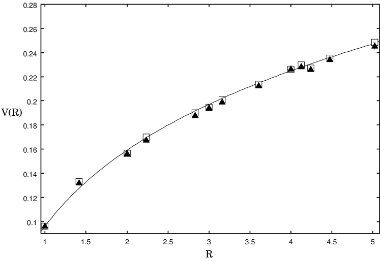
Figure 3: Static quark potentials computed from $R_{xt}$ (solid triangles) and $R_{xy}$ (open squares) as a function of separation $R$ at $\beta=1.306$ and $\Delta\tau=0.5$ using mean field improved gauge action. The potential obtained from $R_{xt}$ has been rescaled by the input anisotropy. The solid line is a fit to the form $V(R)=a+\sigma R+c\mbox{ln}(R)$ to the temporal Wilson loops.

We measured each anisotropy twice, using two different radii $R_{1}$ for subtraction, with fixed $R_{2}$. Setting $R_{2}=4$, we computed the anisotropy with $R_{1}=2$ and $\sqrt{2}$. The two determinations of anisotropy, shown in Table 2, are in excellent agreement. The numerical values of the renormalization of the anisotropy parameter $\eta$ appears to be equal to unity even at large $\beta$. It is seen that for with mean-field improvement the input anisotropy is renormalized by few percent over the range of lattices analyzed here, whereas the measured value of anisotropy is about $15-20\%$ lower than the bare anisotropy with the standard Wilson action. This can be seen from Figure 4 where the renormalization of the anisotropy is plainly visible as a difference in slope of the potentials computed from $R_{xt}$ and $R_{xy}$.

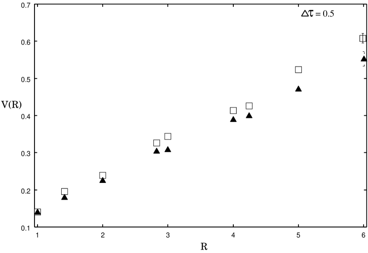
Figure 4: Static quark potentials computed from $R_{xt}$ (solid triangles) and $R_{xy}$ (open squares) at $\beta=1.306$ and $\Delta\tau=0.5$ for standard Wilson action.

Table 2: Measured anisotropy $\xi_{phys.}$ compared to the bare anisotropy $\xi_{0}$ for two actions.

Action	$\xi_{0}$	$\beta$	$\xi_{phys.}$		$\eta=\xi_{phys.}/\xi_{0}$
			$R_{1}=2$	$R_{1}=\sqrt{2}$	$R_{1}=2$	$R_{1}=\sqrt{2}$
Tadpole	0.50	1.306	0.500(1)	0.500(2)	1.00(1)	1.00(4)
Improved		1.443	0.501(2)	0.503(2)	1.00(4)	1.00(4)
		1.592	0.50(2)	0.50(3)	1.00(4)	1.00(6)
		1.892	0.50(5)	0.50(4)	1.0(1)	1.00(8)
	0.40	1.302	0.402(2)	0.401(2)	1.00(4)	1.00(5)
		1.436	0.402(1)	0.403(8)	1.00(2)	1.00(1)
		1.584	0.40(3)	0.40(2)	1.00(6)	1.00(4)
		1.88	0.40(1)	0.40(1)	1.00(7)	1.00(2)
	0.33	1.293	0.335(3)	0.34(1)	1.00(8)	1.03(3)
		1.426	0.33(2)	0.33(1)	1.00(6)	1.00(3)
		1.567	0.33(2)	0.33(1)	1.00(6)	1.00(3)
		1.858	0.33(3)	0.33(1)	1.00(6)	1.00(3)
Wilson	0.50	1.414	0.482(4)	0.471(3)	0.964(8)	0.942(6)
	0.40	1.414	0.336(4)	0.338(3)	0.84(1)	0.845(7)
	0.33	1.414	0.279(5)	0.281(2)	0.83(1)	0.843(6)

Glueball correlation functions $C(\tau)$ were also calculated

$$C(\tau)=\sum_{\tau_{0}}\langle 0\mid\bar{\Phi}_{i}(\tau+\tau_{0})\bar{\Phi}_{i}(\tau_{0})\mid 0\rangle$$ (13)

where $\bar{\Phi}_{i}(\tau)$ is the optimized glueball operator found by a variational technique, following Morningstar and Peardon morn97 and Teper tep99 , from a linear combination of the basic operators $\phi_{i}$,

$$\Phi(\tau)=\sum_{\alpha}v_{i\alpha}\phi_{i\alpha}(\tau)$$ (14)

where the index $\alpha$ runs over the rectangular Wilson loops with dimensions $l_{x}=[n-1,n+1]$, $l_{y}=[n-1,n+1]$ and smearing $n_{s}=[m-1,m+1]$, making 27 operators in all.

The optimized correlation function was fitted with the simple form

$$C_{i}=c_{0}+c_{1}\cosh m_{i}(T/2-\tau)$$ (15)

to determine the glueball mass estimates.

The results for the symmetric and the anti-symmetric glueball masses over the square root of the string tension are shown in Table 3, along with the mean plaquette values at different $\beta$ at $\Delta\tau=1.0$. Figure 5 shows the behaviour of the logarithm of the antisymmetric mass gap over the square root of the string tension as a function of $\beta$. It can be seen that that the ratio scales exponentially to zero in the weak-coupling limit as should be in three-dimensional confining theories. The solid line is a fit to the data over the range $0.916\leq\beta\leq 2.12$. The slope of the data matches the predicted form gof82 , however, the intercept of the scaling curve is large by a factor of 2 (our previous estimates of constant coefficient for standard Wilson action are large by a factor of 5.2 loan02 ). It would be interesting to test the sensitivity of the slope and intercept of the scaling curve by including the radiative corrections.

Figure 5: Logarithmic dimensionless ratio $M/\sqrt{K}\beta^{3/4}$ as a function of $\beta$. The solid curve is the fit to the data for $0.916\leq\beta\leq 2.12$.

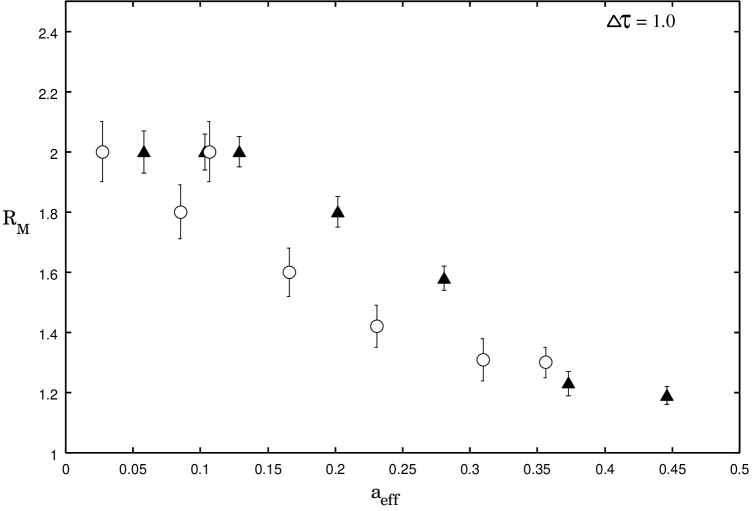
Figure 6: Mass ratio $M_{R}$ against the effective lattice spacing $a_{eff}$ at $\Delta\tau=1.0$. The solid triangles show the estimates for mean field improved gauge action and open circles show the estimates of standard Wilson action.

A plot of mass ratio against the effective lattice spacing $a_{eff}$ loan02 is shown in Figure 6. At weak coupling, the theory is expected to approach a theory of free bosons gof82 so that symmetric state will be composed of two $0^{--}$ bosons and the mass ration should approach two. The mass ratio of the lowest glueball states scale against the effective lattice spacing towards a value close to 2.0, as expected for a theory of free scalar bosons. We note that mass ratio exhibits scaling behaviour, even with the Wilson action loan02 , however, in contrast with the Wilson action, a significant reduction in the errors with tadpole improved action is apparent in the mass gap and the mass ratio.

Table 3: Monte Carlo estimates for the mean plaquette $\langle P\rangle$, the effective lattice spacing, the symmetric and antisymmetric glueball masses $M_{0^{++}}$, $M_{0^{--}}$, for tadpole improved Wilson action at $\Delta\tau=1.0$

Action	$\beta$	$\langle P\rangle$	$a_{eff}$	$M_{0^{++}}/\sqrt{K}$	$M_{0^{--}}/\sqrt{K}$	$R_{M}$
Tadpole	0.917	0.678	0.864	4.0(1)	3.9(1)	1.03(3)
improved	1.243	0.719	0.446	3.83(9)	3.2(1)	1.19(3)
	1.327	0.776	0.373	3.5(2)	2.9(1)	1.23(4)
	1.460	0.797	0.281	3.7(1)	2.34(7)	1.58(4)
	1.613	0.816	0.202	3.6(1)	2.05(2)	1.80(5)
	1.816	0.836	0.129	2.05(4)	0.98(3)	2.00(5)
	1.917	0.844	0.103	2.0(1)	0.99(5)	2.00(6)
	2.168	0.861	0.058	2.19(6)	1.05(2)	2.08(7)
	2.417	0.874
	2.669	0.885
	2.917	0.895
Wilson	1.0	0.475	0.733	3.27(3)	3.1(1)	1.03(6)
	1.35	0.629	0.356	3.6(1)	2.81(9)	1.30(5)
	1.41	0.656	0.310	3.8(1)	2.95(8)	1.31(7)
	1.55	0.704	0.231	4.0(1)	2.81(6)	1.42(7)
	1.70	0.748	0.166	4.03(8)	2.51(2)	1.60(8)
	1.90	0.790	0.107	3.9(1)	1.88(3)	2.0(1)
	2.0	0.806	0.085	3.53(4)	1.96(4)	1.80(9)
	2.5	0.854	0.027	3.1(2)	1.50(8)	2.0(1)

V Summary and Outlook

Mean field improved $U(1)$ lattice gauge theory in (2+1) dimensions was applied to calculations of the static quark potential, the renormalized lattice anisotropy and the scalar glueball masses. We analyzed the mean-link improved action on isotropic and anisotropic lattices and comparisons were made with the simulations of the Wilson action. By comparing the static quark potentials computed from space-like and time-like Wilson loops, we determined the physical anisotropy of the tadpole improved Wilson action. We found that with mean-link improved Wilson action, the bare anisotropy is renormalized by less than a few percent, in contrast with the standard Wilson action, where the measured value of anisotropy is found to be about $15-20\%$ lower than bare anisotropy on the lattices analyzed here. We found that tadpole improvement significantly reduces discretization errors in the static quark potential and the glueball masses. The mass ratio of the two lowest glueball states scales against the effective lattice spacing towards a value close to 2.0, as expected for a theory of free scalar bosons.

We intend to extend PIMC techniques to Symanzik improved $U(1)$ lattice gauge theory. The intention is to study the effects of improvement on the scaling slope, the constant coefficients and scaling behaviour observed in the weak-coupling regime of the theory. We also plan the study the one-loop correction to the anisotropy factor for Symanzik improved $U(1)$ gauge action in three dimensions. We shall report on this work in the near future.

- (1) C. J. Hamer, K. C. Wang and P. F. Price, Phys. Rev. D50, 4693 (1994)
- (2) A.M. Polyakov, Nucl. Phys. B120, 120 (1977)
- (3) A.M. Polyakov, Phys. Lett. B72, 477 (1978)
- (4) H.R. Fiebig and R.M. Woloshyn, Phys. Rev. D42, 3520 (1990)
- (5) T. Banks, R. Myerson and J. Kogut, Nucl. Phys. B129, 493 (1977).
- (6) T. Banks, et al., Phys. Rev. D15, 1111 (1978)
- (7) S.D. Drell, H.R. Quinn, B. Svetitsky and M. Weinstein, Phys. Rev. D19, 619 (1979)
- (8) M. Göpfert and G. Mack, Commun. Math. Phys. 82, 545 (1982)
- (9) M. Loan, M. Brunner, C. Sloggett and C. J. Hamer, Phys. Rev. D68, 034504 (2003)
- (10) J. Snippe, Nucl. Phys. B498, 347 (1997)
- (11) M. García Pérez and P. van Baal, Phys. Lett. B 392, 163 (1997)
- (12) T.R. Klassen, Nucl. Phys. B533, 557 (1998)
- (13) C. Morningstar and M. Peardon, Nucl. Phys. B (Proc. Suppl.) 47, 258 (1996)
- (14) C. Morningstar and M. Peardon, Phys. Rev. D56, 4043 (1997)
- (15) S. Sakai, T. Saito and A. Nakamura, Nucl. Phys. B 584, 528 (2000)
- (16) M. Alford, I.T. Drummond, R.R. Horgan, H. Shanahan and M. Peardon, Phys. Rev. D63, 074501 (2001)
- (17) I.T. Drummond, A. Hart, R.R. Horgan and L.C. Storoni, Phys. Rev. D 66, 094509 (2002)
- (18) J. Engels, F. Karsch and T. Scheideler, Nucl. Phys. B564, 303 (2000)
- (19) N.H. Shakespeare and H.D. Trottier, Phys. Rev. D59, 014502 (1998)
- (20) M. Alford, T.R. Klassen and G.P. Lepage, Phys. Rev D 58, 034503 (1998)
- (21) C. Morningstar, Nucl. Phys. B (Proc. Suppl.) 53, 914 (1997)
- (22) G.P. Lepage, Nucl. Phys. B (Proc. Suppl.) 60, 267 (1998)
- (23) M. Albanese et al., Phys. Letts. B192, 163 (1987)
- (24) M. Teper, Phys. Letts. B183, 345 (1986)
- (25) K. Ishikawa, A. Sato, G. Schierholz and M. Teper, Z. Phys. C21, 167 (1983)
- (26) M. Teper, Phys. Rev. D59, 014512 (1999)